Abstract
Land use regression (LUR) models are used for high-resolution air pollution assessment. These models use independent parameters based on an assumption that these parameters are accurate and invariable; however, they are observational parameters derived from measurements or modeling. Therefore, the parameters are commonly inaccurate, with nonstationary effects and variable characteristics. In this study, we propose a geographically weighted total least squares regression (GWTLSR) to model air pollution under various traffic, land use, and meteorological parameters. To improve performance, the proposed model considers the dependent and independent variables as observational parameters. The GWTLSR applies weighted total least squares in order to take into account the variable characteristics and inaccuracies of observational parameters. Moreover, the proposed model considers the nonstationary effects of parameters through geographically weighted regression (GWR). We examine the proposed model’s capabilities for predicting daily PM2.5 concentration in Isfahan, Iran. Isfahan is a city with severe air pollution that suffers from insufficient data for modeling air pollution with conventional LUR techniques. The advantages of the model features, including consideration of the variable characteristics and inaccuracies of predictors, are precisely evaluated by comparing the GWTLSR model with ordinary least squares (OLS) and GWR models. The values estimated by the GWTLSR model during the spring and autumn are 0.84 and 0.91, respectively. The corresponding average values estimated by the OLS model during the spring and autumn are 0.74 and 0.69, respectively, and the values estimated by the GWR model are 0.76 and 0.70, respectively. The results demonstrate that the proposed functional model efficiently described the physical nature of the relationships among air pollutants and independent variables.
1. Introduction
Urban population growth and industrial development have led to several adverse environmental impacts, including land use change and widespread land degradation [1,2]. These changes contribute to high pollutant concentrations and increased air pollution. Long-term exposure to pollution sources poses the highest risk to human health. Studies have investigated long-term pollution exposure, which can increase mortality rate even if other risk factors, such as smoking, are controlled [3,4]. According to the World Health Organization (WHO), 4% of global mortality can be attributed to air pollution [5]. Due to economic reasons, Asian countries are experiencing greater air pollution levels and higher mortality rates [6,7]. The WHO reported that approximately 4.2 million deaths were due to air pollution in 2016. Every year, worldwide, air pollution is estimated to cause about 16% of mortalities due to lung cancer, 17% due to heart disease, 25% due to brain stroke, and 26% due to respiratory diseases [8,9,10,11].
Due to their minute dimensions, PM2.5 particles can penetrate into various body tissues and cause high pathogenicity [12,13,14]. Urban traffic is the most significant contributor to increased PM2.5 pollution [15,16,17]; industries are another significant source of the increase in PM2.5 concentration. Therefore, populations in highly dense industrial cities are more vulnerable to air pollution-related diseases. For this reason, in such areas, high-resolution estimation of air pollution concentration has become an important issue.
Previous studies have used air pollution monitoring stations to determine levels of exposure. However, considering the variation in pollution concentrations in cities and the costs associated with a large number of monitoring stations, such methods are inefficient at an urban scale [18,19,20]. Alternatively, another group of studies employed portable monitoring devices to explore spatial variations in air pollution; however, these devices pose several limitations when used in large regions [21,22,23]. Due to the difficulties associated with direct measurements of pollutant concentrations, several methods, such as interpolation, dispersion, and LUR have been developed to generate high-resolution data [24,25,26,27]. LUR is a spatial modeling method introduced by Briggs et al. [24]. LUR-based methods entail lower computational costs and have broader applications as compared with dispersion models. Furthermore, they produce small-scale pollutant variations, and thus outperform the interpolation methods for estimating pollution concentration [28].
Models have been developed following the LUR method by considering the pollutant concentration at monitoring stations as the dependent variable and using independent variables such as traffic, land use, and meteorological parameters with the strongest correlations with pollutant concentration [24,29,30,31,32]. Among the various techniques for LUR-based air pollution modeling, there are nonlinear methods with different time scales (daily, monthly, or annual) that use a weighted support vector regression. Such methods consider the relationships among the dependent variable and the independent variables to be constant.
If spatial heterogeneity is present in the observations, an OLS regression yields inaccurate regression coefficients. As a result, studies have considered GWR and mixed-effect models to address this issue [33,34,35,36]. These methods consider the spatial heterogeneity in the observational data and apply a weight matrix to develop the model and to determine the coefficients. The weight matrix is based on the distances between the observation points and monitoring stations. In areas with spatial heterogeneity, the GWR method reveals more details than the OLS method, since the GWR model considers spatial variations at every location, thereby producing more reliable results. However, both of the GWR and OLS models consider the independent variables as accurate and invariable parameters [37].
Solving a regression problem starts by determining a functional model for evaluating the issue. Physical phenomena are described by various functional models specified by dependent and independent variables and their relationships [38]. The primary point when solving a LUR problem is the method used for calculating the functional model coefficients. Most studies have used standard linear regression techniques to develop models for estimating air pollution concentration. The least squares method is commonly used to determine linear regression models’ coefficients by minimizing the root squared error. The coefficient calculation in regression models is performed to improve the accuracy of estimation and modeling of dependent variables. Air pollution modeling commonly considers independent variables such as traffic, meteorological parameters, and land use, all of which are determined by measurement or modeling. Although measurement and modeling inaccuracies and variabilities associated with independent variables have an adverse effect on the estimation accuracy, land use regression models do not take into account the impact of measurement or modeling errors on the independent variables.
In this study, we propose an integrated GWR and a weighted total least squares (WTLS) regression model to improve the existing relations and modeling accuracy. The WTLS method can take into account observational inaccuracies in LUR models. The proposed GWTLSR model introduces random errors into both the design matrix and the observation vector. Hence, the measurement inaccuracies are taken into account when calculating the independent variables. Furthermore, the method’s accuracy and reliability are improved by considering the spatial heterogeneity through GWR. To evaluate the GWTLSR method’s efficiency, a nonlinear weighted LUR model is developed to model the nonlinear relationships among the independent variables, including traffic, meteorological parameters, and land use, and the dependent variable PM2.5 for Isfahan, Iran.
2. Methods and Data
This section starts with an introduction to OLS regression. Next, the development of the OLS-based GWR is described. The capabilities of the WTLS method for estimating regression coefficients are subsequently discussed. Then, it presents how GWR and WTLS are integrated to develop an accurate and reliable model to describe the nonlinear relationship among the independent variables, including traffic, meteorological parameters, and land use on the one hand and PM2.5 concentration on the other hand.
2.1. Ordinary Least Squares Regression
The ordinary least squares method is a statistical technique for estimating the unknown parameters of a linear regression model. OLS minimizes an objective function ∅ representing the sum of squares of the differences between the observed values and the values obtained from the data-fitted model [39]. The objective function to be minimized in the OLS regression is as follows:
where is the error matrix of the observation vector y, if the dimensions of the observation vector are , then, the dimensions of will also be and is the covariance matrix of observations (observations weight matrix). In the OLS model, an equal weight of 1 is assigned to all the observations. Therefore, the covariance matrix in this model is an identity matrix that can be ignored. This model considers that the independent variables are invariable and error-free observations and uses a simple functional model (Equation (2)). The unknown coefficients are calculated based on the method of least squares according to Equation (3) as follows:
In Equation (3), A is the design matrix and x is the vector of unknowns.
2.2. Geographically Weighted Regression
On the basis of the theory of OLS, the GWR method was developed by Fotheringham et al. (2003) to consider spatial heterogeneity. The GWR model is the same as a modified moving windows model. The difference is that the points within the windows of interest are weighted differently, i.e., proportional to the target points [39,40]. In other words, the GWR model provides a local estimation rather than a global estimation of the parameters. Therefore, GWR is one of the best modeling techniques for spatially heterogeneous phenomena. Its general form can be expressed as follows [35,40]:
where represent the coordinates of the th sample in the study space; is the intercept of the linear data-fitted model at location i; to are the local regression coefficients of the 1st to the th independent variables at location I; represents the dependent variable at location i; and is kth independent variable at location i [40].
Since samples (observations) usually outnumber unknowns, the unknown coefficients should be estimated using the least squares method, which is given by:
where is an diagonal matrix whose main diagonal entries represent the weights of the GWR model kernel at location i [40,41]. In this study, a fixed Gaussian-based kernel was used (Equation (6)) as follows:
where is the geographical weight of the kth observation at location i, b is bandwidth, and d is the distance between the location of the kth observation and the location of i.
2.3. GWTLSR
The regression coefficients in both of the GWR and OLS models are calculated by minimizing the sum of squared errors. These models use the standard least squares method. These models only consider errors in the observation vector, and the design matrix (A) is assumed to be accurate and error free. In air pollution modeling, PM2.5 concentration and also the values of independent variables are obtained by measurement or modeling. Hence, there are errors-in-variables (EIV). The ordinary least squares method does not yield accurate solutions for such problems. Weighted total least squares can be used to solve the previously mentioned problem, introduced by Markovsky et al. in 2006 [42]. Due to the widespread use of least squares methods in various scientific fields, different formulations have been proposed for the WTLS method. In this study, an OLS-based formulation for the total least squares [43] was applied to develop the land use regression model.
Contrary to OLS, the WTLS model considers errors in the design matrix and the observation vector. Therefore, the total least squares method can improve modeling accuracy if random errors influence the coefficient matrix. In air pollution modeling, the design matrix entries are the independent variables that include modeled traffic variables, land use parameters derived from aerial images and field surveys, and meteorological parameters measured at synoptic stations. Each of these parameters has an independent measurement accuracy. As a result, WTLS enables taking the independent variables’ inaccuracies into account along with the dependent variable’s inaccuracies and can be used more efficiently to determine the model coefficients.
Similar to OLS, the total least squares method minimizes the sum of squared differences between observational values and the data-fitted model’s values. The difference is that it must also simultaneously minimize design matrix errors along with minimizing the observation vector errors. To solve the WTLS problem, this study used Lagrange multipliers to minimize the objective function given by the following:
where is an identity matrix, λ represents the vector of Lagrange multipliers, is an vector of design matrix errors, and indicates the vector of unknown.
Taking the first derivative of Equation (7) with respect to each of the main values, one obtains the following four equations:
By simultaneously solving the set of Equations (8)–(11), the , , , and values are obtained as follows:
The operator in Equation (13) reshapes the mn vector to an m n matrix. The relations for total least squares and ordinary least squares are similar in form, as indicated by Equation (15). In Equation (15), is the design matrix, represents the covariance matrix, and is the observation vector. Here, the aim is to calculate to determine the modeling coefficients. Considering the general forms of these equations, the equation can be solved using an iterative mechanism and determining the unknowns’ initial values by employing OLS.
A hybrid method that consolidates WTLS and GWR is proposed to consider spatial heterogeneity, variable characteristics, and inaccuracies in air pollution modeling variables. This model applies WTLS to determine the GWR coefficients. The general formula used in the model has the following form:
where is the observation matrix consisting of the dependent variables, A is the design matrix carrying the values of the independent variables as well as a column of coefficient 1 representing the intercept of the model, x represents the coefficient values of the independent variable, and is the random errors of the design matrix , which is defined as follows:
where is the value of the th independent variable in location i.
where is the value of the dependent variable in location i.
where is the coefficient of the th variable and is the intercept, located at .
where the operator, , converts an vector to an matrix; is the matrix of the measured weights in the GWR model; and is the weight matrix of the independent variables. and are defined as follows:
where represents the measurement accuracy (variances) associated with the th independent variable in the th sample, and the values in Equation (22) are the measured weights in GWR based on the neighboring distance.
Once the covariance matrices are determined, Equation (15) and total least squares are used to calculate the model coefficients following an iterative process (Figure 1).
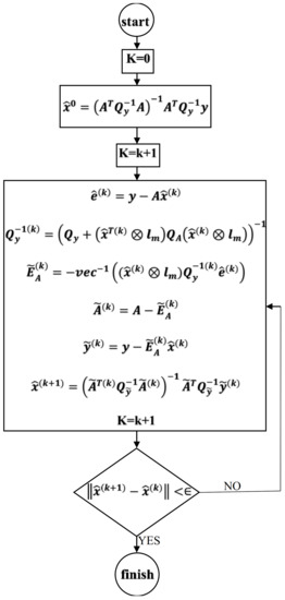
Figure 1.
Schematic algorithm of the hybrid model.
2.4. Comparison of Regression Models
The Akaike information criterion () coefficient, the coefficient of determination, the root mean squared error (RMSE), and the mean absolute error (MAE) were employed to assess the regression models’ performance. is calculated as follows:
where , , and are the sample size, bandwidth, and standard deviation of the model, respectively. Each row of the matrix that contains independent variables is determined according to Equation (24) [44]:
In Equations (25)–(27), n is the sample size, is i-th station observed to be dependent variable, is the mean values of the independent variable, and is the estimated value of the dependent variable.
Moreover, two statistical metrics, the probability of false alarm (POF) and the probability of detection (POD) [45,46], were applied to evaluate the regression model’s performance for estimating PM2.5 concentration.
where a is the number of events in which both observed and estimated PM2.5 concentrations are higher than the 90th percentile (successful predictions); b is the number of events in which the estimated PM2.5 concentration is lower than the 90th percentile, whereas the observed PM2.5 concentration is higher than the 90th percentile (unsuccessful predictions); c is the number of events in which the estimated PM2.5 concentration is higher than the 90th percentile, whereas the observed PM2.5 concentration is lower than the 90th percentile (wrong alarms). In a perfect prediction, POD equals one, and POF equals zero.
2.5. Study Area and Data Preparation
With a population of more than 2.1 million, Isfahan is one of the most populous and polluted industrial cities in central Iran (Figure 2). It is home to many industrial units as one of Iran’s industrial hubs. According to previous studies, traffic, residential land use, and nonresidential land use are responsible for 76%, 11%, and 13% of emissions in Isfahan on a daily basis, respectively [47]. Therefore, in this study, the LUR model was developed based on these predictors to estimate the PM2.5 pollutant concentration.
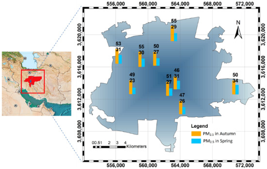
Figure 2.
Distribution of air pollution monitoring stations in zone 39N of the universal Transverse Mercator (UTM) coordinate system and seasonal PM2.5 concentrations.
The study area included nine monitoring stations and the target pollutant concentrations were measured in one-hour intervals from 2017 to 2019 during the spring and autumn. The seasons are considered according to calendar seasons. The calculated average daily concentrations were used for modeling purposes. After checking the quality of the measured data at each station and removing the biased samples, on average, each station contained 260 and 240 measurements in spring and autumn, respectively (Figure 2).
The independent variables used in this study were traffic, land use, and meteorological parameters, as they have the most significant effect on PM2.5 concentration in Isfahan [48,49]. These variables are described as follows.
- The meteorological parameters included temperature, humidity, precipitation, pressure, and wind speed measured by the Isfahan Weather Forecast Organization at the synoptic stations. The measurements were taken in three-hour intervals during the spring and autumn from 2017 to 2019. The daily average of the measured value was considered to be an independent variable at each station.
- The traffic data obtained from the Isfahan Municipality included traffic volume from a four-stage transportation model. First, the hourly traffic counts were determined for sample days during the spring and autumn from 2017 to 2019. Second, they were extracted in buffers around the monitoring stations of 150, 300, 600, and 1200 m radius. Finally, the buffers with the highest correlation were eventually kept in the model.
- The land use data were derived from a 2019 map (scale = 1:2000). The original land use classes were reclassified into residential and non-residential classes. Subsequently, buffers of 100, 200, and 500 m radius were used to estimate the relevant independent variables.
In order to improve modeling accuracy, the significant independent variables were selected from all variables using a two-stage process. The first stage used Pearson’s correlation coefficient to choose the variables bearing the strongest correlation to the independent variables (Figure 3). In the second stage, various combinations of the selected variables were applied to develop OLS-based models. The variables with p-values more than 0.05 were ignored. Finally, the variables having the most significant effect on the were selected to develop the OLS, GWR, and GWTLSR models.
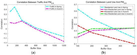
Figure 3.
Correlation coefficients between PM2.5 concentration and independent variables ((a) traffic and (b) land use) for various buffers in spring and autumn.
Figure 3 shows the correlation coefficients between the independent variables and PM2.5 concentration in the spring and autumn. On the one hand, the results showed that, in the autumn, the following variables had the highest correlation with PM2.5 concentration: the 1200 m buffer traffic volume with a negative relationship and residential and non-residential land use in the 100 m and 500 m buffers with a direct relationship. Among the meteorological parameters, temperature with a negative relationship and pressure directly bore the highest correlations with PM2.5 concentration. In the spring, on the other hand, the variables bearing the highest correlation with PM2.5 concentration were residential and non-residential land use in the 100 m and 500 m buffers and traffic in a 150 m buffer, all with a direct effect. In addition, temperature and pressure were among the variables bearing the highest correlation with PM2.5 concentration with positive and negative relationships. The temperature relationship with PM2.5 was considerably more significant in autumn than spring due to lower temperatures and thermal inversion.
3. Results and Discussion
Figure 4 presents the distribution of RMSE in the OLS model using combinations of one to five independent variables, which are most closely correlated with PM2.5. As shown in Figure 4, once the number of independent variables increased from one to five, the value of RMSE decreased accordingly. Therefore, a combination of five independent variables was eventually used in the final model. The selected independent variables applied in the spring were traffic in the 150 m buffer, residential and non-residential land use in the 100 m and 500 m buffers, respectively, temperature, and pressure. The selected independent variables applied in the autumn were traffic in the 300 m buffer, residential and non-residential land use both in the 200 m buffers, temperature, and pressure.
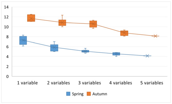
Figure 4.
Distribution of root mean square error (RMSE) in autumn and spring with respect to the number of independent variables.
In order to examine the selected independent variables, the p-value and variance inflation factor (VIF) index of the selected variables have been presented (Table 1). The closer the VIF index values of each independent variable are to one, the better the variable is selected in the model. There are no multiple alignments among the chosen variables.

Table 1.
Comparison of p-value and variance inflation factor (VIF) values in selected independent variables.
Table 2 shows the results of the three models for the spring and autumn. Model performance was evaluated by cross-validation. Given the number of stations in the study area, the models were validated by the leave-one-out cross-validation method. One station was left out from the observations at each stage in this method, and the models were developed using the remaining stations. According to the number of monitoring stations in the study area, the data used were divided into nine sections. At each stage, observations of one station were considered to be testing data and the remaining stations were considered to be training data. This process was repeated nine times and, in each step, observations of one station were considered to be test data. The modeling accuracy was determined at the end of the process based on the mean accuracy of all stages. The mean values of RMSE and MAE for the test and training data sets and of the models are shown in Table 2. The results demonstrated the superior performance of the GWTLSR method as compared with the other modeling techniques. A reduction in the coefficient accompanied the improved performance as compared with the other models. This reduction indicated the high computational efficiency of the proposed model. The accuracy was improved without any substantial increase in computational complexity. The absence of a significant difference between the validation results for the two seasons demonstrated the proposed model’s stability.
Table 2.
Results of the three models in spring and autumn for test and training datasets.
Figure 5 shows that the integrated GWTLSR model explains 0.82 and 0.92 of the total variances of PM2.5 in the spring and autumn, respectively. While the corresponding values were, respectively, 0.74 and 0.69 for the OLS model and 0.7 and 0.76 for the GWR model. The higher . coefficient of the proposed model showed that it was superior in accuracy and covered the dependent variable distribution more broadly. The results presented in Table 1 and Figure 5 show that considering inaccuracy, varying characteristics, and nonstationary effects of independent variables simultaneously led to performance improvement of the GWTLSR model as compared with conventional models used in previous research.
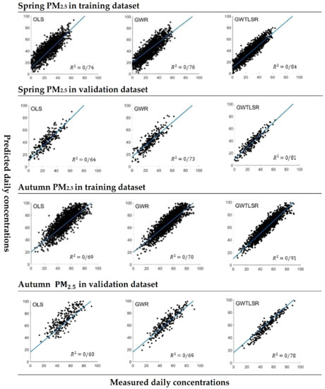
Figure 5.
Scatter plots of estimated (y axis) against observed (x axis) for PM2.5 (μg/m3) for the test and training data sets.
In order to evaluate the significance of the accuracy difference in the studied models, one-way analysis of variance (ANOVA) with a confidence interval of 0.95% was used. The results of the analysis show the significant difference in accuracy among the studied models.
Figure 6 shows the average POD (%) values of GWTLSR for estimating PM2.5 concentration which was higher than the other models, in addition, the average GWTLSR POF (%) values were lower than the two other models for estimating PM2.5 concentration.
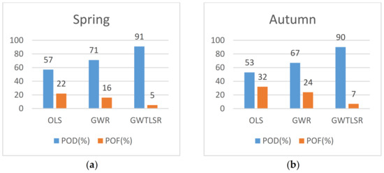
Figure 6.
The probability of detection (POD (%)) and probability of false alarm (POF (%)) for estimation of PM2.5 in (a) spring and (b) autumn.
Figure 7 presents the PM2.5 concentrations obtained from the GWTLSR model for the spring and autumn. Moreover, it shows the differences between the estimated and observed PM2.5 concentrations in the spring and autumn at monitoring stations for the three modeling methods. The maximum differences obtained by the integrated model in the spring and autumn are 2.23 and 1.74, respectively. The corresponding differences are, respectively, 3.54 and 4.20 for the OLS model and 2.63 and 3.74 for the GWR model. In the OLS and GWR models, the differences between the estimated and observed concentrations increase as the pollutant concentration increased. However, the corresponding difference in the proposed model is not significant. Thus, it can be concluded that the performance of the proposed model is less affected by the mean and variance of the dependent parameters.
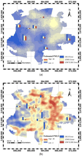
Figure 7.
Estimated PM2.5 concentrations in (a) spring and (b) autumn, using the GWTLSR model and the models’ error at monitoring stations.
As shown in Figure 7, the Moran’s I Index was applied to examine the spatial autocorrelation of the models’ errors. Table 3 presents the Moran’s I Index values of the proposed model as −0.10 and −0.12, with p-values equal to 0.89 and 0.98 for the spring and autumn, respectively. Thus, the distribution of errors in the GWTLSR model is random. It can be concluded that the errors in the GWTLSR are not dependent on the monitoring station’s location due to the consideration of variable characteristics and nonstationary effects of parameters.
Table 3.
Spatial autocorrelation (Moran’s I) of the model’s error.
4. Conclusions
This study proposed a geographically weighted total least squares regression (GWTLSR) model for high-resolution mapping of air pollution. The proposed model simultaneously considered the independent and dependent variables to be observational parameters. It could also consider the nonstationary effects of the parameters affecting pollutant concentration. These model features enabled effective air pollution modeling through available parameters with spatial heterogeneity and different measurement accuracy levels.
In the development of the proposed model, the WTLS was applied to calculate the GWR coefficients. Random errors were introduced to both the design matrix and the observation vector by using the WTLS method. As a result, the GWTLSR model estimates the results by considering measurement inaccuracies of the independent variables. Furthermore, spatial heterogeneity is taken into account in the proposed model by using GWR.
To assess the GWTLSR model’s performance, a nonlinear weighted LUR model was developed to model the nonlinear relationships among traffic, meteorological parameters, and land use as the independent variables, and PM2.5 as the dependent variable for spring and autumn in Isfahan, Iran. The proposed integrated model’s benefits were investigated by comparing it with two conventional LUR models, namely OLS and GWR. These conventional models consider the independent variables to be invariable and accurate. As a result, the covariance matrix of observations only includes the covariance of the dependent variable. In contrast, the covariance matrix in the GWTLSR model contains both dependent and independent variables’ values. The results show that despite the insignificant differences between the performances of the OLS and GWR models, the GWTLSR model’s accuracy increased significantly. In addition, comparing the results for the spring and autumn demonstrated that the variables’ values and variance had less influence on the proposed model’s performance than that of the other two. In conclusion, although all these methods are developed based on the OLS theory, the GWTLSR model is more compatible with the variables’ nature. Therefore, the proposed model can significantly contribute to enhance air pollution modeling.
Author Contributions
Conceptualization, B.T.; formal analysis, A.M. and B.T.; investigation, A.M. and B.T.; methodology, A.M. and B.T.; software, A.M. and B.T.; supervision, B.T. and K.D.; writing—original draft, A.M.; writing—review and editing, B.T. and K.D. All authors have read and agreed to the published version of the manuscript.
Funding
This research received no external funding.
Institutional Review Board Statement
Not applicable.
Informed Consent Statement
Not applicable.
Data Availability Statement
The datasets used and analyzed during the current study are available from the corresponding author on reasonable request. The code used during the current study are available from the corresponding author on reasonable request.
Conflicts of Interest
The authors declare no conflict of interest.
References
- Ganivet, E. Growth in human population and consumption both need to be addressed to reach an ecologically sustainable future. Environ. Dev. Sustain. 2019, 22, 4979–4998. [Google Scholar] [CrossRef]
- Riley, W.J.; Matson, P.A. Nloss: A mechanistic model of denitrified N2O and N2 evolution from soil. Soil Sci. 2000, 165, 237–249. [Google Scholar] [CrossRef]
- Chen, J.; Hoek, G. Long-term exposure to PM and all-cause and cause-specific mortality: A systematic review and meta-analysis. Environ. Int. 2020, 143, 105974. [Google Scholar] [CrossRef] [PubMed]
- Dockery, D.W.; Pope, C.A.; Xu, X.; Spengler, J.D.; Ware, J.H.; Fay, M.E.; Ferris, B.G.; Speizer, F.E. An Association between Air Pollution and Mortality in Six U.S. Cities. N. Engl. J. Med. 1993, 329, 1753–1759. [Google Scholar] [CrossRef]
- Cohen, A.J.; Anderson, H.R.; Ostro, B.; Pandey, K.D.; Krzyzanowski, M.; Künzli, N.; Gutschmidt, K.; Pope, A.; Romieu, I.; Samet, J.M.; et al. The Global Burden of Disease Due to Outdoor Air Pollution. J. Toxicol. Environ. Health Part A 2005, 68, 1301–1307. [Google Scholar] [CrossRef]
- Balakrishnan, K.; Dey, S.; Gupta, T.; Dhaliwal, R.S.; Brauer, M.; Cohen, A.J.; Stanaway, J.; Beig, G.; Joshi, T.K.; Aggarwal, A.N.; et al. The impact of air pollution on deaths, disease burden, and life expectancy across the states of India: The Global Burden of Disease Study 2017. Lancet Planet. Health 2019, 3, e26–e39. [Google Scholar] [CrossRef]
- Zhao, H.; Geng, G.; Zhang, Q.; Davis, S.J.; Li, X.; Liu, Y.; Peng, L.; Li, M.; Zheng, B.; Huo, H.; et al. Inequality of household consumption and air pollution-related deaths in China. Nat. Commun. 2019, 10, 4337. [Google Scholar] [CrossRef]
- Alfaro-Moreno, E.; Martínez, L.; García-Cuellar, C.; Bonner, J.C.; Murray, J.C.; Rosas, I.; Rosales, S.P.D.; Osornio-Vargas, A.R. Biologic effects induced in vitro by PM10 from three different zones of Mexico City. Environ. Health Perspect. 2002, 110, 715–720. [Google Scholar] [CrossRef]
- Miller, M.R.; Newby, E.D. Air pollution and cardiovascular disease: Car sick. Cardiovasc. Res. 2019, 116, 279–294. [Google Scholar] [CrossRef]
- Osornio-Vargas, A.R.; Bonner, J.C.; Alfaro-Moreno, E.; Martínez, L.; García-Cuellar, C.; Rosales, S.P.-D.-L.; Miranda, J.; Rosas, I. Proinflammatory and cytotoxic effects of Mexico City air pollution particulate matter in vitro are dependent on particle size and composition. Environ. Health Perspect. 2003, 111, 1289–1293. [Google Scholar] [CrossRef]
- WHO. 2016. Available online: https://www.who.int/gho/phe/outdoor_air_pollution/burden_text/en/ (accessed on 13 November 2019).
- Brehmer, C.; Norris, C.; Barkjohn, K.K.; Bergin, M.H.; Zhang, J.; Cui, X.; Teng, Y.; Zhang, Y.; Black, M.; Li, Z.; et al. The impact of household air cleaners on the oxidative potential of PM2.5 and the role of metals and sources associated with indoor and outdoor exposure. Environ. Res. 2020, 181, 108919. [Google Scholar] [CrossRef]
- Geiser, M.; Kreyling, W.G. Deposition and biokinetics of inhaled nanoparticles. Part. Fibre Toxicol. 2010, 7, 2. [Google Scholar] [CrossRef]
- Möller, W.; Felten, K.; Sommerer, K.; Scheuch, G.; Meyer, G.; Meyer, P.; Häussinger, K.; Kreyling, W.G. Deposition, Retention, and Translocation of Ultrafine Particles from the Central Airways and Lung Periphery. Am. J. Respir. Crit. Care Med. 2008, 177, 426–432. [Google Scholar] [CrossRef]
- Askariyeh, M.H.; Zietsman, J.; Autenrieth, R. Traffic contribution to PM2.5 increment in the near-road environment. Atmos. Environ. 2020, 224, 117113. [Google Scholar] [CrossRef]
- Morawska, L.; Wang, H.; Ristovski, Z.; Jayaratne, E.R.; Johnson, G.; Cheung, H.C.; Ling, X.; He, C. JEM Spotlight: Environmental monitoring of airborne nanoparticles. J. Environ. Monit. 2009, 11, 1758–1773. [Google Scholar] [CrossRef]
- Saremi, P. The Role of Traffic Culture Making in Air Pollution Reduction in Metropolitans of Developing Countries. Int. J. Transp. Eng. Traffic Syst. 2020, 6, 42–54. [Google Scholar]
- Hoek, G.; Beelen, R.; de Hoogh, K.; Vienneau, D.; Gulliver, J.; Fischer, P.; Briggs, D. A review of land-use regression models to assess spatial variation of outdoor air pollution. Atmos. Environ. 2008, 42, 7561–7578. [Google Scholar] [CrossRef]
- Jerrett, M.; Arain, M.A.; Kanaroglou, P.; Beckerman, B.; Potoglou, D.; Sahsuvaroglu, T.; Morrison, J.; Giovis, C. A review and evaluation of intraurban air pollution exposure models. J. Expo. Sci. Environ. Epidemiology 2005, 15, 185–204. [Google Scholar] [CrossRef]
- Miller, K.A.; Siscovick, D.S.; Sheppard, L.; Shepherd, K.; Sullivan, J.H.; Anderson, G.L.; Kaufman, J.D. Long-Term Exposure to Air Pollution and Incidence of Cardiovascular Events in Women. N. Engl. J. Med. 2007, 356, 447–458. [Google Scholar] [CrossRef]
- Adams, M.D.; Massey, F.; Chastko, K.; Cupini, C. Spatial modelling of particulate matter air pollution sensor measurements collected by community scientists while cycling, land use regression with spatial cross-validation, and applications of machine learning for data correction. Atmos. Environ. 2020, 230, 117479. [Google Scholar] [CrossRef]
- Morley, D.W.; Gulliver, J. A land use regression variable generation, modelling and prediction tool for air pollution exposure assessment. Environ. Model. Softw. 2018, 105, 17–23. [Google Scholar] [CrossRef]
- Yu, X.; Ivey, C.; Huang, Z.; Gurram, S.; Sivaraman, V.; Shen, H.; Eluru, N.; Hasan, S.; Henneman, L.; Shi, G.; et al. Quantifying the impact of daily mobility on errors in air pollution exposure estimation using mobile phone location data. Environ. Int. 2020, 141, 105772. [Google Scholar] [CrossRef] [PubMed]
- Briggs, D.J.; Collins, S.; Elliott, P.; Fischer, P.; Kingham, S.; Lebret, E.; Pryl, K.; Van Reeuwijk, H.; Smallbone, K.; Van Der Veen, A. Mapping urban air pollution using GIS: A regression-based approach. Int. J. Geogr. Inf. Sci. 1997, 11, 699–718. [Google Scholar] [CrossRef]
- Chen, S.; Yuval; Broday, D.M. Re-framing the Gaussian dispersion model as a nonlinear regression scheme for retrospective air quality assessment at a high spatial and temporal resolution. Environ. Model. Softw. 2020, 125, 104620. [Google Scholar] [CrossRef]
- Jerrett, M.; Arain, M.A.; Kanaroglou, P.; Beckerman, B.; Crouse, D.; Gilbert, N.; Brook, J.R.; Finkelstein, N.; Finkelstein, M.M. Modeling the Intraurban Variability of Ambient Traffic Pollution in Toronto, Canada. J. Toxicol. Environ. Health Part A 2007, 70, 200–212. [Google Scholar] [CrossRef]
- Liu, X.; Wang, X.; Zou, L.; Xia, J.; Pang, W. Spatial imputation for air pollutants data sets via low rank matrix completion algorithm. Environ. Int. 2020, 139, 105713. [Google Scholar] [CrossRef]
- Marshall, J.D.; Nethery, E.; Brauer, M. Within-urban variability in ambient air pollution: Comparison of estimation methods. Atmospheric Environ. 2008, 42, 1359–1369. [Google Scholar] [CrossRef]
- Ainslie, B.; Steyn, D.; Su, J.; Buzzelli, M.; Brauer, M.; Larson, T.; Rucker, M. A source area model incorporating simplified atmospheric dispersion and advection at fine scale for population air pollutant exposure assessment. Atmospheric Environ. 2008, 42, 2394–2404. [Google Scholar] [CrossRef]
- Janssen, N.A.; van Vliet, P.H.; Aarts, F.; Harssema, H.; Brunekreef, B. Assessment of exposure to traffic related air pollution of children attending schools near motorways. Atmospheric Environ. 2001, 35, 3875–3884. [Google Scholar] [CrossRef]
- Just, A.C.; Wright, R.O.; Schwartz, J.; Coull, B.A.; Baccarelli, A.A.; Tellez-Rojo, M.M.; Moody, E.; Wang, Y.; Lyapustin, A.; Kloog, I. Using high-resolution satellite aerosol optical depth to estimate daily PM2.5 geographical distribution in Mexico City. Environ. Sci. Technol. 2015, 49, 8576–8584. [Google Scholar] [CrossRef]
- Liu, W.; Li, X.; Chen, Z.; Zeng, G.; Leon, T.; Liang, J.; Huang, G.; Gao, Z.; Jiao, S.; He, X.; et al. Land use regression models coupled with meteorology to model spatial and temporal variability of NO2 and PM10 in Changsha, China. Atmos. Environ. 2015, 116, 272–280. [Google Scholar] [CrossRef]
- Basu, B.; Alam, S.; Ghosh, B.; Gill, L.; McNabola, A. Augmenting limited background monitoring data for improved performance in land use regression modelling: Using support vector regression and mobile monitoring. Atmospheric Environ. 2019, 201, 310–322. [Google Scholar] [CrossRef]
- Brunsdon, C.; Fotheringham, A.S.; Charlton, M.E. Geographically Weighted Regression: A Method for Exploring Spatial Nonstationarity. Geogr. Anal. 2010, 28, 281–298. [Google Scholar] [CrossRef]
- Fotheringham, A.S.; Charlton, M.; Brunsdon, C. Measuring Spatial Variations in Relationships with Geographically Weighted Regression. In Recent Developments in Spatial Analysis; Springer: Berlin/Heidelberg, Germany, 1997; pp. 60–82. [Google Scholar]
- Son, Y.; Osornio-Vargas, Á.R.; O’Neill, M.S.; Hystad, P.; Texcalac-Sangrador, J.L.; Ohman-Strickland, P.; Meng, Q.; Schwander, S. Land use regression models to assess air pollution exposure in Mexico City using finer spatial and temporal input parameters. Sci. Total. Environ. 2018, 639, 40–48. [Google Scholar] [CrossRef]
- Song, W.; Jia, H.; Li, Z.; Wang, C. Detecting urban land-use configuration effects on NO2 and NO variations using geographically weighted land use regression. Atmos. Environ. 2019, 197, 166–176. [Google Scholar] [CrossRef]
- Mikhail, M.E.; Ackermann, F.E. Observations and Least Squares; University Press of America: Lanham, MD, USA, 1982. [Google Scholar]
- Xiao, L.; Lang, Y.; Christakos, G. High-resolution spatiotemporal mapping of PM2.5 concentrations at Mainland China using a combined BME-GWR technique. Atmos. Environ. 2018, 173, 295–305. [Google Scholar] [CrossRef]
- Fotheringham, A.S.; Brunsdon, C.; Charlton, M. Geographically Weighted Regression: The Analysis of Spatially Varying Relationships; John Wiley & Sons: Hoboken, NJ, USA, 2003. [Google Scholar]
- Yu, X.; Wang, Y.; Niu, R.; Hu, Y. A Combination of Geographically Weighted Regression, Particle Swarm Optimization and Support Vector Machine for Landslide Susceptibility Mapping: A Case Study at Wanzhou in the Three Gorges Area, China. Int. J. Environ. Res. Public Health 2016, 13, 487. [Google Scholar] [CrossRef]
- Markovsky, I.; Rastello, M.L.; Premoli, A.; Kukush, A.; Van Huffel, S. The element-wise weighted total least-squares problem. Comput. Stat. Data Anal. 2006, 50, 181–209. [Google Scholar] [CrossRef]
- Amiri-Simkooei, A.; Jazaeri, S. Weighted total least squares formulated by standard least squares theory. J. Géod. Sci. 2012, 2, 113–124. [Google Scholar] [CrossRef]
- Lu, B.; Charlton, M.; Harris, P.; Fotheringham, A.S. Geographically weighted regression with a non-Euclidean distance metric: A case study using hedonic house price data. Int. J. Geogr. Inf. Sci. 2014, 28, 660–681. [Google Scholar] [CrossRef]
- Kang, D.; Eder, B.K.; Stein, A.F.; Grell, G.A.; Peckham, S.E.; McHenry, J. The New England Air Quality Forecasting Pilot Program: Development of an Evaluation Protocol and Performance Benchmark. J. Air Waste Manag. Assoc. 2005, 55, 1782–1796. [Google Scholar] [CrossRef] [PubMed][Green Version]
- Xu, L.; Chen, N.; Zhang, X.; Chen, Z.; Hu, C.; Wang, C. Improving the North American multi-model ensemble (NMME) precipitation forecasts at local areas using wavelet and machine learning. Clim. Dyn. 2019, 53, 601–615. [Google Scholar] [CrossRef]
- Zarrabi, A.; Mohammadi, J.; Abdollahi, A. Evaluation of mobile and stationary sources of Isfahan air pollution. Geography 2010, 26, 151–164. [Google Scholar]
- Tashayo, B.; Alimohammadi, A. Modeling urban air pollution with optimized hierarchical fuzzy inference system. Environ. Sci. Pollut. Res. 2016, 23, 19417–19431. [Google Scholar] [CrossRef]
- Tashayo, B.; Alimohammadi, A.; Sharif, M. A Hybrid Fuzzy Inference System Based on Dispersion Model for Quantitative Environmental Health Impact Assessment of Urban Transportation Planning. Sustainability 2017, 9, 134. [Google Scholar] [CrossRef]


Publisher’s Note: MDPI stays neutral with regard to jurisdictional claims in published maps and institutional affiliations. |
© 2021 by the authors. Licensee MDPI, Basel, Switzerland. This article is an open access article distributed under the terms and conditions of the Creative Commons Attribution (CC BY) license (https://creativecommons.org/licenses/by/4.0/).