Abstract
Climate change stressors like rising and warmer seas, increased storms and droughts, and acidifying oceans are rapidly threatening coastal zones, which are the world’s most densely inhabited places. This research assesses the effects of Palm Jumeirah Island (PJI) construction on its surrounding water quality and temperature, using Landsat-7 and 8 spectral and thermal bands for the years 2001, 2014, 2016, 2019, and 2020. To aid in this goal, the changes in water spectral reflectance was observed and interpreted, based on previous research and measurements, to discover the correlation between water quality and its spectral reflectance. Then, the sea surface temperature (SST) was calculated for the years under review and changes in water temperature were evaluated. Finally, the Green Normalized Difference Vegetation Index (GNDVI) and the Normalized Difference Turbidity Index (NDTI) were calculated to estimate water chlorophyll levels and water turbidity, respectively, and changes were observed and interpreted for the time period under review. The present study showed that the PJI construction not only increased the water reflectance in the 0.5–0.8 µm of wavelength, which can be considered to be the increase of suspended sediments and chlorophyll but the water temperature also increased by 7.5 °C during the 19 years. In addition, a gradual increase in the values of GNDVI (by 0.097–0.129) and NDTI (by 0.118~0.172) were observed. A drop in chlorophyll and suspended sediment spectral reflectance and GNDVI and NDTI values were also observed in 2020 compared to 2019 which can be attributed to the 63 to 82% decrease in tourists in Dubai in 2020 as a result of the COVID-19 pandemic. This study aims to draw attention to environmental issues by clarifying the effect of creating artificial islands in the sea and our analysis and results are a suitable reference for specialized hydrological and environmental studies based on spectral information and distance measurements, as presented in this paper.
1. Introduction
Coastal zones, which are the world’s most densely populated locations, are quickly being threatened by climate change stressors such as rising and warmer seas, greater storms, and droughts [1], and acidifying oceans. Despite the fact that local human activities have long had an impact on coastal zones, it is still unknown how local human effects and climate change stressors may combine to endanger coastal ecosystems [2]. Coastal areas, as well as the food they produce, provide a significant contribution to the national economy and food supply in the United Arab Emirates. In recent years, the substitution of shrimp farming for agriculture in coastal areas has been a paradigm shift, owing to increased shrimp production and changes in land use/land cover [3,4,5]. Human interventions, such as establishing shrimp [6] farms, not caring for drained swamps [7], aquaculture, commercial navigation, or using areas as sewage and industrial waste disposal sites [8], have caused an increase in the salinity of water near the shores [9]. The loss of soil fertility, a lack of fresh water for drinking, and the increased risk to public health are all consequences of seawater salinity (particularly near coasts) [6,10,11,12,13]. Because a rise in these pollutants might disrupt the ecology and harm human health and aquatic creature habitats, for those who live on beaches near the ocean, monitoring water-soluble chemicals (including water salinity) is crucial [9,14,15,16].
Assessing water quality resources is necessary for water purification. Water quality considers a body of water’s thermal, physical, chemical, and biological qualities. It is a metric for determining whether or not water is fit for human consumption or recreational usage. Water quality is difficult to define since its use varies so much. For example, water characteristics that are acceptable in agriculture irrigation, differ from those which make water fit for human consumption [17]. Furthermore, water quality is frequently connected to consumer safety. Drinking water can include a broad range of chemical and microbiological pollutants, some of which can have significant health consequences for users. Understanding the types of contaminants that might enter the water supply and how they get there, is critical to ensuring water safety [17]. Water quality is also linked to discharges from urban, agricultural, and industrial sources. In addition, fecal contamination of surface water is a worldwide hazard caused by urban waste flows, and urban stormwater runoff has been demonstrated to contribute to surface water quality by harboring substantial amounts of fecal bacteria [18].
Traditional methods for measuring saline levels are both costly and time-consuming, requiring extensive primary data collection and laboratory testing [19,20,21,22]. So, the remote sensing approach, which has previously been demonstrated to be an effective way of monitoring water quality, might be an alternate tool to make the monitoring process more comfortable and successful [22,23,24,25,26]. Furthermore, Landsat data sets provide diverse satellite images, making monitoring and change detection easier and more efficient than primary data collection. In this respect, water’s optical properties are relevant because they are affected by a variety of factors, including the concentration and features of suspended particles, dissolved solids, and other organic materials [27,28,29]. An effective monitoring strategy might be utilized based on the link between the optical features of water and the band values of the Landsat data series [19,29,30].
For various places, several investigators from across the world have developed many approaches for detecting water quality metrics using Landsat images [9,26,29,31,32,33,34,35]. Gonzalez-Marquez et al. (2018) demonstrated that Landsat-8 Operational Land Imager (OLI) images may be used to analyze water quality metrics such as phosphate concentrations, electrical conductivity, total suspended particles, turbidity, and pH in Mexico’s coastal zones. In Iraq’s Al-Huwaizah wetland, Landsat-8 OLI imagery was also shown to be capable of monitoring salinity. In another study, to build a monitoring strategy for the Mekong delta of Vietnam, Vu et al. (2018) focused on the link between in-situ salinity level data and Landsat-8 (OLI) band values [36]. Water quality metrics, such as suspended sediments, turbidity, chlorophyll-a, and others, may be mapped using Landsat-5 TM. To analyze the association between band values and field level parameter values, Nas et al. (2010) created regression models for these parameters using 28 band compositions [9].
Bugnot et al. (2018) used Landsat-5 (TM) and 7 (ETM+) to monitor and analyze environmental changes in Australian estuaries at the watershed level. Another water quality measure that may be determined using Landsat images is suspended solid concentration (SSC). To identify SSC from Landsat pictures, Shahzad et al. (2018) and Montaner et al. (2014) built empirical models. According to Chang et al. (2017), remote sensing techniques may be the most practical method of monitoring and regulating water quality [37]. Turbidity, total suspended particles, and heavy metals such as iron, zinc, copper, chromium, lead, and cadmium may all be detected using Landsat spectral band data [9,21]. It may also be used to measure chlorophyll-a levels and water clarity. Using linear regression analysis, Vignolo et al. (2006) created a model to detect water quality index from Landsat-7 ETM band data, notably the blue and green bands. This research also shows that Landsat pictures’ blue and green bands may be used to accurately determine water quality [38].
Morshed et al. (2016) used Landsat-7 ETM+ data to create a regression equation to identify soil salinity in coastal Bangladesh. Ferdous and Rahman (2018) likewise looked at the use of Landsat-5 TM to identify the region’s soil water content [39]. Ferdous et al. (2019) have advocated using Landsat-8 OLI pictures to monitor the content of water using the total dissolved solids (TDS) index in surface water in coastal Bangladesh [40]. As a result of beach closures, reduced fishing, or deterioration of drinking water supplies, water quality has a significant impact on both public health and the economy [11]. Agricultural run-off and industrial wastewater, on the other hand, contribute to eutrophication processes, resulting in phytoplankton buildup. The increase in nutrient levels encourages excessive plant growth, which causes the water to become murky, has an impact on fish populations, and speeds up algal blooms [41,42]. Consideringly, this study aims to study the effect of Palm Jumeirah Island (PJI) construction in the Persian Gulf on the surrounding waters, to give a scientific view of the extent of changes in the water profile arising from the construction of the island. Since thermal remote sensing is a helpful technology for detecting thermal changes in marine systems that might alter the biological production rate [43,44], this study assesses the changes in PJI’s surrounding water temperature during the 19 years from before the island existed, to its completion and subsequent growth. Additionally, by examining the correlation between parameters calculated from the characteristics of the water, the effect or effectiveness of each parameter, on/from other parameters, are shown. This study can be used as a scientific reference of water features for hydrologists conducting research in this area in the future, and also to monitor the trend of water changes during PJI’s construction.
2. Materials and Methods
2.1. Study Area
The Study area is the PJI located on the Persian Gulf islands around Dubai and its surrounding waters. PJI is located on 25°07′09.2′′ N 55°07′49.3′′ E of geographic longitude and latitude coordinates (Figure 1). It has an area of 7.6 km2 [45] and homes a population of 78,000 [46]. The Palm Jumeirah is the first of a series of man-made islands off Dubai’s shore; the project began in 2001 [47] and was completed in 2008, adding 56 km to the coastline [48]. The project involved adding 120 million cubic meters of sand and 7 million tons of rock to the sea [46]. An offshore crescent barrier enclosing the island, with a total length of 11 km, was built at the same time to defend the island from wave attacks [49].
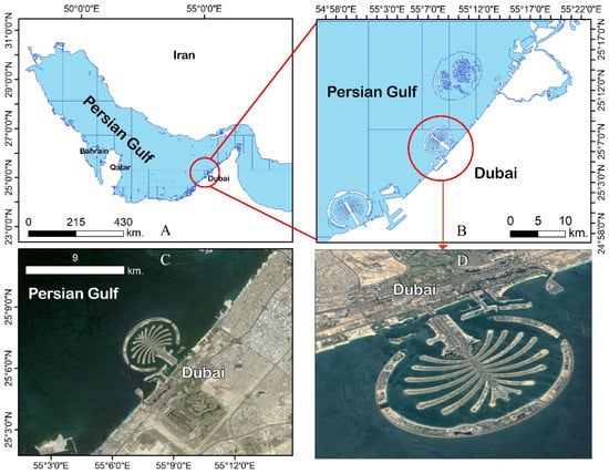
Figure 1.
(A) Location of PJI, (B) location in zoom, (C) Landsat-8 RGB color image (2020), and (D) Google Earth image (2021).
2.2. Data Collection
For the present study, Landsat-7/Enhanced Theme Mapper Plus (ETM+) and Landsat-8/Operational Land Imager and the Thermal Infrared Sensor (OLI/TIRS) images in path 160 and row 043 were used. These images were selected for the years 2001, 2014, 2016, 2019, and 2020, based on the closest images and the presence of suitable images without error and cloud for processing. The images were derived from the United States Geological Survey (USGS) portal. More details about the images used are provided in Table 1. August is the hottest month of the year in Dubai; to meet the images criteria, we tried to use images for this month. A gap was unavoidable as no perfect-quality images were found from August, or in the months before or after, in the period from 2001 to 2013.

Table 1.
Details about the Landsat datasets used in this research.
2.3. Data Preprocessing
After collecting the images, they were corrected radiometrically and atmospherically through ENVI software and the Fast Line-of-sight Atmospheric Analysis of Spectral Hypercubes (FLAASH) algorithm, which is recommended for atmospheric correction over ocean or water body images. Then each image’s spectral reflectance was analyzed through the transition of years from 2001 to 2014, 2016, 2019, and 2020. Then water indices were calculated to show and compare the changes in water content through changes in the indices values. Finally, the Sea Surface Temperature (SST) was calculated for the study period, to monitor changes in water temperature.
2.4. Derivation of Image Spectral Characteristics
To monitor water quality, remote sensing techniques rely on the capacity to measure changes caused by compounds in the spectral signature backscattered from water. Suspended sediments (turbidity), thermal releases, algae (i.e., chlorophylls and carotenoids), dissolved organic matter, chemicals (i.e., nutrients, pesticides, and metals), pathogens, aquatic vascular plants, and oils are all major factors affecting water quality in water bodies across the landscape [50]. The energy spectrum of reflected solar and/or emitting thermal radiation from surface waters is changed by suspended sediments, algae, dissolved organic matter, oils, aquatic vascular plants, and thermal releases, which can be studied using remote sensing techniques [50]. Thus, by extracting the spectral behavior of the water around PJI in the studied time series, this study investigates the spectral reflectance changes to the waters of this region, over the studied years for each pixel. The pixels studied on water reflection as samples are as shown in Figure 2. The samples were selected in the same position for all years.
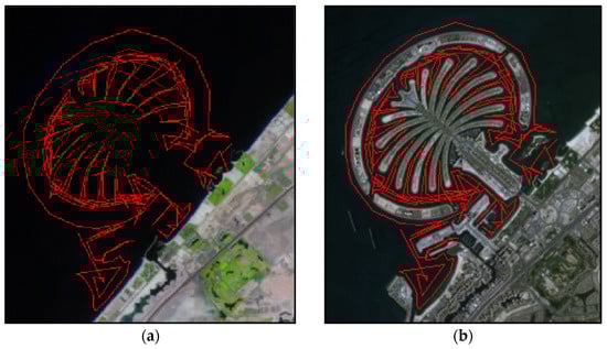
Figure 2.
Study examples of changes in the spectral behavior of water around PJI (a) before PJI (2001), and (b) after PJI (in 2020).
2.5. Calculation of the Sea Surface Temperature (SST)
2.5.1. Calculation of the SST for ETM+ Sensor Single-Band
In order to calculate the SST from the ETM+ sensor thermal band (6th band), first of all, the DN (Digital Number) image of the thermal band converted radiance was calculated using Equation (1):
where is spectral radiance (watts/m2·str·µm)), is spectral radiance which is correlated with DNMAX (watts/m2·str·µm)), is spectral radiance, which is correlated with DNMIN, and is the minimum value of DN (1 or 0 based on LPGS or NLAPS Product, respectively). Then, an atmospheric correction was performed using the thermal atmospheric correction algorithm [51,52] in ENVI software. Then, thermal bands were converted to the effective temperature value using Equation (2):
where is the effective temperature (°C), and are the calibration constants 2 and 1 for the thermal band Table 2. The thermal band used in this study is band 62 of Landsat-7, which is recommended as the more effective band for the SST calculation [53].
Table 2.
The calibration constants of the ETM+ thermal band.
2.5.2. Calculating the SST for the TIRS Multi-Band
For the 11µm and 12µm channels, the multi-channel SST (MCSST) algorithm has been employed most often for SST retrieval from satellite data [54,55,56,57,58,59,60,61]. Although the single-window method was used in previous studies [62,63,64], the multi-window method has also been used in several studies [65,66,67,68,69,70,71,72,73]. To calculate the SST for the TIRS images (for the years 2014, 2016, 2019, and 2020) Equation (3) was used [73]:
where , , are the regression coefficients given in Table 3 and and are brightness temperature at 11 µm and 12 µm (in Celsius) which are the 10th and 11th bands of Landsat-8 (TIRS satellite).
Table 3.
MCSST correlation coefficients [73].
Additionally, to ensure that the SST is not affected by other climatic variables, information on air temperature, wind speed, and relative humidity of the study area was extracted [74] on the day and hour of imaging and with the help of statistical parameters R2, p-Value, and Significance-F, significance between these parameters were obtained with the calculated SST for the study area.
2.6. Calculation of Water Indices
2.6.1. The Green Normalized Difference Vegetation Index (GNDVI)
The present study used the GNDVI index to evaluate the changes in the chlorophyll content of the water because the index is extremely sensitive to changes in chlorophyll content, which is inversely proportional to the water nitrogen content [75,76,77]. The GNDVI maps were calculated using Equation (4) [75]:
where is the near-infrared band which is the Landsat-8 (OLI) 5th and the Landsat-7 (ETM+) 4th bands and is the band with a 0.54~0.57 µm wavelength range which is the green band (Landsat-8 (OLI) 3rd and Landsat-7 (ETM+) 2nd bands).
2.6.2. The Normalized Difference Turbidity Index (NDTI)
The NDTI index was calculated for using remote sensing data to evaluate the turbidity of water in ponds and inland waters [77,78]. The NDTI maps were calculated using Equation (5) [78]:
where is the red band which is the Landsat-8 (OLI) 4th and the Landsat-7 (ETM+) 3rd bands.
2.6.3. Statistical Analysis
In order to statistically evaluate the parameters and indicators used in this study, using data matrices, the relationship and significance of the indicators over time per pixel were calculated using correlation coefficients and their R2 using Microsoft excel software.
Figure 3 schematically shows the research method.
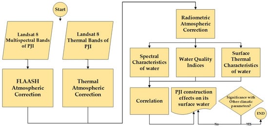
Figure 3.
The flowcharts of the present research methods.
3. Results and Discussion
3.1. Changes in Water Spectral Characteristics
The study aims to evaluate the effects of island construction, specially PJI, Dubai, on its surrounding water reflectance, content, and temperature using remote sensing data to observe the changes during the years 2001 (before there was the island), 2014, 2016, 2019, and 2020. The results indicate that the water reflectance of the water around the island has been changed during the study period (Figure 4).
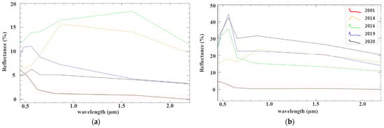
Figure 4.
(a) Maximum and (b) mean reflectance of water surrounding PJI for the years 2001, 2014, 2016, 2019, and 2020.
Figure 4a clearly illustrates that the maximum reflectance has shifted to shorter wavelengths during the time period under review. The maximum water reflectance was 0.8~0.9 µm in 2014, and it had shifted to 0.5~0.6 µm in 2019 and 2020. Although the maximum reflectance of surrounding water was 1.6~1.7 µm in 2016, two peaks in 0.8~0.9 µm (near to 2014) and a high value of reflectance in 0.5~0.6 µm (near 2019 and 2020) are observed. It is while the reflectance was at 0.483 µm in 2001 that it shows an observable shift of the maximum reflectance to shorter wavelengths. Figure 4b also shows an almost regular trend with a regular increase of mean of water reflectance in 0.5~0.6 µm and 0.6~0.7 µm of wavelength from 2001 to 2016.
The comparison of the maximum water reflectance between 2014 and 2016 (Figure 4a) also clearly shows an increase in 0.8~0.9 µm in 2016, and the same increase has accrued between 2019 and 2020 in 0.5~0.6 µm of wavelength; the difference is that the maximum reflectance of 2019, in 0.5~0.6 µm, was much higher than in 2020. In the same trend as Figure 4a, the mean of water reflectance in 0.5~0.6 µm of wavelength was higher in 2019 than in 2020 (Figure 4b). This trend is significant according to Figure 5 in the perception of the amount of substances in water.
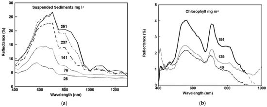
Figure 5.
The relationship between reflectance and wavelength as affected by the (a) concentration of suspended sediments [43] and (b) chlorophyll concentrations [79].
3.2. Water Temperature Changes
Remote sensing mapping of absolute temperatures reveals geographical and temporal patterns of thermal releases that may be used to manage thermal releases. In this study, the assessment of water temperature was performed using SST algorithms. Thus, the SST maps for 2001, 2014, 2016, 2019, and 2020, and the overall changes to the maps, were calculated from ETM+ and TIRS thermal bands as shown in Figure 6.
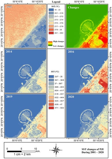
Figure 6.
The calculated SST maps for 2001, 2014, 2016, 2019, and 2020 of PJI together with the overall map changes during this period.
As shown in Figure 6, the island’s surrounding water surface temperature has gradually warmed since the island was built in 2001. The change map shows this change visually (Figure 6). The statistics of the SST maps indicate that the mean of the SST around the island has continuously increased from 27.5 °C in 2001 to 34.5 °C in 2014, 34.9 °C in 2016 and 2019, and finally, 35 °C in 2020. The maximum and minimum SST also increased constantly from 28 and 26.7 °C, respectively, in 2001 to 36.7 and 34.3 °C, respectively, in 2020 (Figure 7).
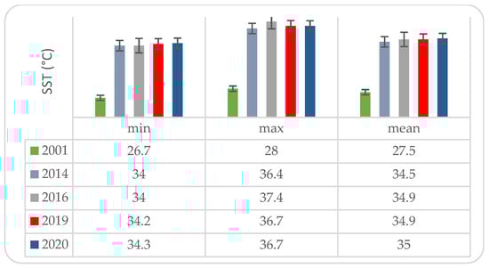
Figure 7.
Statistics of the SST maps for 2001, 2014, 2016, 2019, and 2020 of PJI.
The results also show that there was no significance between the SST obtained in the study area and the climatic parameters of areas such as air temperature, wind speed, and relative humidity (Table 4).
Table 4.
Statistical values of the relationships between different climatic parameters and the SST in the study area.
3.3. Assessment of Water Indices
Since many studies have used spectral indices in order to assess water quality, content, etc., in the present study we calculated some indices to find out the effects of the island’s construction on the water quality in the PJI area. To achieve this goal, GNDVI and NDTI were calculated to give a clear view of the changes that have taken place in this region, during the study period. The maps of changes of these indices during the relevant time period are shown in Figure 8.
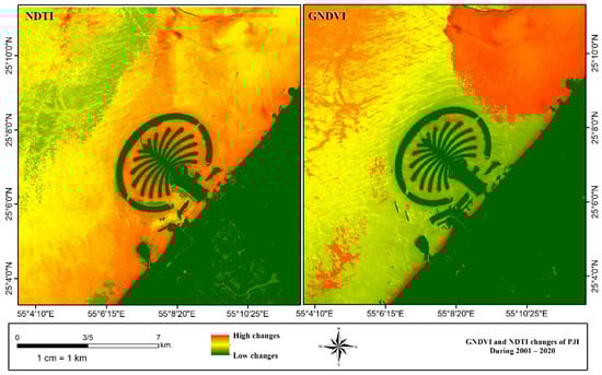
Figure 8.
The GNDVI and NDTI change maps for PJI’s surrounding water from 2001 to 2020.
The mean outputs of the GNDVI and NDTI calculations, which are more acceptable for deriving water parameters, are presented in Figure 9.
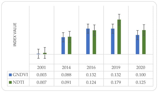
Figure 9.
Results of the GNDVI and NDTI calculations from PJI’s surrounding water (mean).
Based on the indices results (Figure 9), GNDVI permanently increased from 0.003 in 2001 to 0.132 in 2019 in the water surrounding PJI. The NDTI results also confirm a similar trend around the island, it has had increased from 0.007 in 2001 to 0.179 in 2019. In 2020, a small decrease was observed in the GNDVI and NDTI results from 2019 (by 0.032 and 0.054, respectively) to 0.1 and 0.125, respectively.
The results show that increases in GNDVI, NDTI, and SST in the surrounding waters of PJI have been observed since building the island. However, the results of the statistical analysis of the matrix of changes in the pixels of the water area around PJI indicate that the highest significance and correlation was between the GNDVI results and the SST, with a correlation and R2 of 85.3% and 80.76%, respectively. After this, the highest correlation and significance was observed between the NDTI results and the green band reflectance (GBR), with a correlation of 49.7% and an R2 of 36.08%. Then came the correlation and significance between the GNDVI and NDTI results, with a correlation and R2 of 39.1% and 44.81%, respectively, and NDTI and SST, with a correlation and R2 of 34.5% and 40.77%, respectively. Finally, the least correlation and significance were obtained between GNDVI and GBR, with less than 20%, and SST and GBR, with less than 12% Table 5.
Table 5.
Statistical relation between PJI water surrounding indices (sorted by descending).
4. Discussion
The maximum reflectance has changed to shorter wavelengths over time, indicating that the maximum reflectance has altered. As a result, in 2014, the maximum water reflectance was 0.8~0.9 µm, whereas, in 2019 and 2020, it was 0.5~0.6 µm. Even though the highest depth of surrounding water was 1.61.7 m in 2016, two peaks in 0.8~0.9 µm (near 2014) and a high value of reflectance in 0.5~0.6 µm (near 2019 and 2020) have been detected. The results depict an observable shift of the maximum reflectance to shorter wavelengths, while the reflectance was 0.483 µm in 2001. From 2001 to 2016, the results also demonstrate an extremely consistent trend of increasing mean water reflectance in the 0.5~0.6 and 0.6~0.7 µm wavelength ranges. Significant connections have been described between suspended sediments and brightness or reflectance measured on satellite sensors using spectral bands or combinations of bands before [43,50]. So the increase in PJI’s surrounding water reflectance in 0.5~0.6 µm of wavelength, reveals the increase in the concentration of suspended sediments in the water due to the island’s construction. Increased reflection at 0.5~0.65 µm wavelengths may also indicate an increase in chlorophyll [79] at the water surface. In addition, the maximum water reflectance between 2014 and 2016 (Figure 4a) indicates a definite rise in 0.8~0.9 µm in 2016 and a similar increase in 0.5~0.6 µm wavelength between 2019 and 2020. The difference is that the maximum reflectance of 2019 in 0.5~0.6 µm was significantly higher than in 2020 (Figure 4b). Considering that the inhabitants of this island are of seventy different nationalities [80], the COVID-19 lockdown has led to a decrease in travel and human activity in the region, so this reduction in the maximum reflectance may be due to a 68 to 82% fall in tourism to Dubai in 2020, due to the COVID-19 pandemic [81]. In this regard, many prior studies have proven the effect of lockdown in the COVID-19 era [82,83,84] and foreign direct investment [85] on environmental pollution.
According to the results, the SST of the waters around PJI has increased by a maximum of 27.2% over 19 years. While earlier Landsat satellite studies used a mono-window technique with single-channel data for SST retrieval [62,63,64], the Landsat 8 OLI/TIRS allowed for the use of a split-window method with multi-channel data for the SST estimate [65,66,67,68,69,70,71,72,73]. Thus, comparing the following years with 2001 (27.5 °C), in 2014, this temperature had a difference of 25.5% to 34.5 °C, in 2016 and 2019, a difference of 26.7% to 34.9 °C, and finally, in 2020, a difference of 27.2% to 35 °C. When human impact alters the temperature of a body of water, thermal pollution occurs. So, in addition to water reflectance, considering that no significant relationship was observed in the results between the SST values and the climatic variables of air temperature, wind speed, and relative humidity, the change in SST in the water surrounding PJI is clearly the effect of the island’s construction. The results show that the increase in the GNDVI and NDTI was up to a maximum of 4203% and 2321%, respectively. This amount was recorded from 0.0003 in 2001, with a 2764.7% difference, with 0.0088 in 2014, with a 4203% difference, with 0.132 in 2016 and 2019, and with a 3139.2% difference, with 0.1 in 2020. These differences may be because the creation of the island has increased the water chlorophyll, as the indices are sensitive to chlorophyll content changes [76,77]. Further, as an estimation for water turbidity, the NDTI results clearly show an increase in turbidity in the water surrounding PJI. In 2020, both the GNDVI and NDTI decreased somewhat (by 0.032 and 0.054, respectively) to 0.1 and 0.125, respectively. This, as mentioned before, could be due to a decrease of 68% to 82% of tourists in Dubai in 2020.
In addition, the results obtained from the study with respect to the correlation and significance between indices (and GBR), indicate that the highest correlation and R2 (above 80%) was between GNDVI and SST. This can be a good indication of the relationship between these two indicators and the effect of the increased GNDVI values (increasing water chlorophyll content) and the increased water surface temperature. Next, NDTI and GBR values, with a correlation coefficient of 49.7% and an R2 of 36.08%, have a relatively high correlation and significance, which clearly indicates the relationship between these two parameters and the increase in the reflection in the green wavelength and the increase in the NDTI values during the study period and after the construction of PJI. The third significant correlation, with the correlation coefficient of 39.1% and R2 of 44.81%, was between NDTI and GNDVI, which can indicate the effect of these two parameters on each other during the statistical period and the consequent increase in both of these parameters (increased chlorophyll and suspended sediments) after PJI’s fabrication. In addition, NDTI and SST, with a correlation coefficient of 34.5% and R2 of 40.77%, indicate a relatively significant relationship between these two parameters and could indicate that this index is similar to GNDVI but with a lower coefficient that has increased the water surface temperature. Both GNDVI and SST values had a low correlation and significance (less than 20% and 12%, respectively) with GBR, indicating that these two parameters were not directly related to or affected by GBR.
5. Conclusions
This study aimed to investigate the effect of PJI’s construction on the quality of its surrounding waters from 2001 (before island construction) to 2020. According to the results, the construction of this island has changed the spectral characteristics of the surrounding water and has increased water reflection in the range of 0.5 to 0.8 µm. This increase can be considered to be an increase in suspended particles and chlorophyll in the water. The construction also raised the average water temperature by 7.5 °C, over 19 years. The results obtained from the study of GNDI and NDTI also showed an increase in the values of these indices from 2001 to 2019, which can be considered to be an increase in the water’s chlorophyll content and water turbidity. The study found a slight drop in the values of these indicators in 2020, which is likely due to a sharp decline (68 to 82%) in tourists in Dubai in 2020 (due to the COVID-19 pandemic). The study results were obtained using Landsat-7/ETM+ and Landsat-8 OLI/TIRS images to assess the quality and temperature of the seawater in the study area around the island. These results can be used as a reference for more specialized studies by experts in the field of hydrology, using the remote sensing data which is presented in this research.
Author Contributions
Conceptualization, M.M.; data curation, M.M. and H.R.G.M.; funding acquisition, H.Z.; methodology, M.M., H.R.G.M. and I.R.; software, M.M., H.R.G.M. and I.R.; supervision, H.R.G.M., H.O. and H.Z.; validation, H.R.G.M., H.O. and H.Z.; visualization, M.M.; Writing—review & editing, M.M. and H.Z. All authors have read and agreed to the published version of the manuscript.
Funding
This study is supported by Shanghai Municipal Science and Technology Commission within the international cooperation framework of the Youth Scientists from the ‘One Belt and One Road’ countries.
Institutional Review Board Statement
Not Applicable.
Informed Consent Statement
Not Applicable.
Data Availability Statement
Contact to mohammadmoghaddam@stu.yazd.ac.ir or irousta@yazd.ac.ir.
Acknowledgments
I.R. is deeply grateful to his supervisor (Haraldur Olafsson, Professor of Atmospheric Sciences, Institute for Atmospheric Sciences-Weather and Climate, and the Department of Physics, University of Iceland, and Icelandic Meteorological Office (IMO)), for his great support, kind guidance, and encouragement.
Conflicts of Interest
The authors declare no conflict of interest.
References
- Rousta, I.; Olafsson, H.; Moniruzzaman, M.; Ardö, J.; Zhang, H.; Mushore, T.D.; Shahin, S.; Azim, S. The 2000–2017 drought risk assessment of the western and southwestern basins in Iran. Modeling Earth Syst. Environ. 2020, 6, 1201–1221. [Google Scholar] [CrossRef]
- He, Q.; Silliman, B.R. Climate change, human impacts, and coastal ecosystems in the Anthropocene. Curr. Biol. 2019, 29, R1021–R1035. [Google Scholar] [CrossRef] [PubMed]
- Rahman, M.T.U.; Tabassum, F.; Rasheduzzaman, M.; Saba, H.; Sarkar, L.; Ferdous, J.; Uddin, S.Z.; Islam, A.Z. Temporal dynamics of land use/land cover change and its prediction using CA-ANN model for southwestern coastal Bangladesh. Environ. Monit. Assess. 2017, 189, 565. [Google Scholar] [CrossRef]
- Moniruzzaman, M.; Thakur, P.K.; Kumar, P.; Ashraful Alam, M.; Garg, V.; Rousta, I.; Olafsson, H. Decadal Urban Land Use/Land Cover Changes and Its Impact on Surface Runoff Potential for the Dhaka City and Surroundings Using Remote Sensing. Remote Sens. 2021, 13, 83. [Google Scholar] [CrossRef]
- Mansourmoghaddam, M.; Rousta, I.; Zamani, M.; Mokhtari, M.H.; Karimi Firozjaei, M.; Alavipanah, S.K. Study and prediction of land surface temperature changes of Yazd city: Assessing the proximity and changes of land cover. J. RS GIS Nat. Resour. 2021, 12, 1–27. [Google Scholar]
- Basar, A. Water security in coastal region of Bangladesh: Would desalination be a solution to the vulnerable communities of the sundarbans? Bangladesh E J. Sociol. 2012, 9, 31. [Google Scholar]
- Baten, M.A.; Seal, L.; Lisa, K.S. Salinity intrusion in interior coast of Bangladesh: Challenges to agriculture in south-central coastal zone. Am. J. Clim. Change 2015, 4, 248. [Google Scholar] [CrossRef]
- Le Tixerant, M. Dynamique des Activités Humaines en Mer Côtière. Application à la Mer d’Iroise; Université de Bretagne occidentale-Brest: Brest, France, 2004. [Google Scholar]
- Ferdous, J.; Rahman, M.T.U. Developing an empirical model from Landsat data series for monitoring water salinity in coastal Bangladesh. J. Environ. Manag. 2020, 255, 109861. [Google Scholar] [CrossRef]
- Nahian, M.A.; Ahmed, A.; Lázár, A.N.; Hutton, C.W.; Salehin, M.; Streatfield, P.K.; Chadwick, O.; Renaud, F. Drinking water salinity associated health crisis in coastal Bangladesh. Elem. Sci. Anthr. 2018, 6, 2. [Google Scholar] [CrossRef]
- Rahman, M.T.U.; Ferdous, J. Detection of environmental degradation of satkhira district, Bangladesh through remote sensing indices. In Proceedings of Global Civil Engineering Conference; Springer: Singapore, 2017; pp. 1053–1066. [Google Scholar]
- Miao, R.; Liu, Y.; Wu, L.; Wang, D.; Liu, Y.; Miao, Y.; Yang, Z.; Guo, M.; Ma, J. Effects of long-term grazing exclusion on plant and soil properties vary with position in dune systems in the Horqin Sandy Land. Catena 2022, 209, 105860. [Google Scholar] [CrossRef]
- Zhao, T.; Shi, J.; Lv, L.; Xu, H.; Chen, D.; Cui, Q.; Jackson, T.J.; Yan, G.; Jia, L.; Chen, L. Soil moisture experiment in the Luan River supporting new satellite mission opportunities. Remote Sens. Environ. 2020, 240, 111680. [Google Scholar] [CrossRef]
- Zhao, T.; Shi, J.; Entekhabi, D.; Jackson, T.J.; Hu, L.; Peng, Z.; Yao, P.; Li, S.; Kang, C.S. Retrievals of soil moisture and vegetation optical depth using a multi-channel collaborative algorithm. Remote Sens. Environ. 2021, 257, 112321. [Google Scholar] [CrossRef]
- Zhang, K.; Chao, L.-J.; Wang, Q.-Q.; Huang, Y.-C.; Liu, R.-H.; Hong, Y.; Tu, Y.; Qu, W.; Ye, J.-Y. Using multi-satellite microwave remote sensing observations for retrieval of daily surface soil moisture across China. Water Sci. Eng. 2019, 12, 85–97. [Google Scholar] [CrossRef]
- Zhang, K.; Ali, A.; Antonarakis, A.; Moghaddam, M.; Saatchi, S.; Tabatabaeenejad, A.; Chen, R.; Jaruwatanadilok, S.; Cuenca, R.; Crow, W.T. The sensitivity of North American terrestrial carbon fluxes to spatial and temporal variation in soil moisture: An analysis using radar-derived estimates of root-zone soil moisture. J. Geophys. Res. Biogeosci. 2019, 124, 3208–3231. [Google Scholar] [CrossRef]
- Cherif, E.K.; Salmoun, F.; Mesas-Carrascosa, F.J. Determination of bathing water quality using thermal images Landsat 8 on the west coast of Tangier: Preliminary results. Remote Sens. 2019, 11, 972. [Google Scholar] [CrossRef]
- Selvakumar, A.; Borst, M. Variation of microorganism concentrations in urban stormwater runoff with land use and seasons. J. Water Health 2006, 4, 109–124. [Google Scholar] [CrossRef] [PubMed]
- Abdelmalik, K. Role of statistical remote sensing for Inland water quality parameters prediction. Egypt. J. Remote Sens. Space Sci. 2018, 21, 193–200. [Google Scholar] [CrossRef]
- Morshed, M.M.; Islam, M.T.; Jamil, R. Soil salinity detection from satellite image analysis: An integrated approach of salinity indices and field data. Environ. Monit. Assess. 2016, 188, 119. [Google Scholar] [CrossRef]
- Swain, R.; Sahoo, B. Mapping of heavy metal pollution in river water at daily time-scale using spatio-temporal fusion of MODIS-aqua and Landsat satellite imageries. J. Environ. Manag. 2017, 192, 1–14. [Google Scholar] [CrossRef]
- Shahzad, M.I.; Meraj, M.; Nazeer, M.; Zia, I.; Inam, A.; Mehmood, K.; Zafar, H. Empirical estimation of suspended solids concentration in the Indus Delta Region using Landsat-7 ETM+ imagery. J. Environ. Manag. 2018, 209, 254–261. [Google Scholar] [CrossRef]
- Le, C.; Hu, C.; Cannizzaro, J.; Duan, H. Long-term distribution patterns of remotely sensed water quality parameters in Chesapeake Bay. Estuar. Coast. Shelf Sci. 2013, 128, 93–103. [Google Scholar] [CrossRef]
- Dona, C.; Chang, N.-B.; Caselles, V.; Sánchez, J.M.; Camacho, A.; Delegido, J.; Vannah, B.W. Integrated satellite data fusion and mining for monitoring lake water quality status of the Albufera de Valencia in Spain. J. Environ. Manag. 2015, 151, 416–426. [Google Scholar] [CrossRef] [PubMed]
- Binding, C.E.; Greenberg, T.A.; Watson, S.B.; Rastin, S.; Gould, J. Long term water clarity changes in North America’s Great Lakes from multi-sensor satellite observations. Limnol. Oceanogr. 2015, 60, 1976–1995. [Google Scholar] [CrossRef]
- Bugnot, A.; Lyons, M.; Scanes, P.; Clark, G.; Fyfe, S.; Lewis, A.; Johnston, E. A novel framework for the use of remote sensing for monitoring catchments at continental scales. J. Environ. Manag. 2018, 217, 939–950. [Google Scholar] [CrossRef] [PubMed]
- Hellweger, F.; Schlosser, P.; Lall, U.; Weissel, J. Use of satellite imagery for water quality studies in New York Harbor. Estuar. Coast. Shelf Sci. 2004, 61, 437–448. [Google Scholar] [CrossRef]
- Pavelsky, T.M.; Smith, L.C. Remote sensing of suspended sediment concentration, flow velocity, and lake recharge in the Peace-Athabasca Delta, Canada. Water Resour. Res. 2009, 45. [Google Scholar] [CrossRef]
- González-Márquez, L.C.; Torres-Bejarano, F.M.; Rodríguez-Cuevas, C.; Torregroza-Espinosa, A.C.; Sandoval-Romero, J.A. Estimation of water quality parameters using Landsat 8 images: Application to Playa Colorada Bay, Sinaloa, Mexico. Appl. Geomat. 2018, 10, 147–158. [Google Scholar] [CrossRef]
- Mallick, J.; Hasan, M.A.; Alashker, Y.; Ahmed, M. Bathymetric and geochemical analysis of lake al-saad, abha, kingdom of saudi arabia using geoinformatics technology. J. Geogr. Inf. Syst. 2014, 6, 440. [Google Scholar] [CrossRef]
- Hasab, H.A.; Ahmad, A.; Marghany, M.; Ziboon, A.R. Landsat TM-8 Data for retrieving salinity in AL-HUWAIZAH marsh, south of IRAQ. J. Teknol. 2015, 75, 201–206. [Google Scholar] [CrossRef][Green Version]
- Nas, B.; Ekercin, S.; Karabörk, H.; Berktay, A.; Mulla, D.J. An application of Landsat-5TM image data for water quality mapping in Lake Beysehir, Turkey. Water Air Soil Pollut. 2010, 212, 183–197. [Google Scholar] [CrossRef]
- Chen, X.; Quan, Q.; Zhang, K.; Wei, J. Spatiotemporal characteristics and attribution of dry/wet conditions in the Weihe River Basin within a typical monsoon transition zone of East Asia over the recent 547 years. Environ. Model. Softw. 2021, 143, 105116. [Google Scholar] [CrossRef]
- Huo, W.; Li, Z.; Wang, J.; Yao, C.; Zhang, K.; Huang, Y. Multiple hydrological models comparison and an improved Bayesian model averaging approach for ensemble prediction over semi-humid regions. Stoch. Environ. Res. Risk Assess. 2019, 33, 217–238. [Google Scholar] [CrossRef]
- Zhao, X.; Xia, H.; Pan, L.; Song, H.; Niu, W.; Wang, R.; Li, R.; Bian, X.; Guo, Y.; Qin, Y. Drought monitoring over Yellow River basin from 2003–2019 using reconstructed MODIS land surface temperature in Google Earth Engine. Remote Sens. 2021, 13, 3748. [Google Scholar] [CrossRef]
- Vu, N.N.; Trung, L.V.; Van, T.T. Development of the Statistical Model for Monitoring Salinization in the Mekong Delta of Vietnam Using Remote Sensing Data and In-Situ Measurements. Proceedings 2018, 2, 565. [Google Scholar] [CrossRef]
- Chang, N.-B.; Bai, K.; Chen, C.-F. Integrating multisensor satellite data merging and image reconstruction in support of machine learning for better water quality management. J. Environ. Manag. 2017, 201, 227–240. [Google Scholar] [CrossRef]
- Vignolo, A.; Pochettino, A.; Cicerone, D. Water quality assessment using remote sensing techniques: Medrano Creek, Argentina. J. Environ. Manag. 2006, 81, 429–433. [Google Scholar] [CrossRef] [PubMed]
- Ferdous, J.; Rahman, M.T.U.; Ghosh, S.K. Detection of total dissolved solids from Landsat 8 OLI image in coastal Bangladesh. In Proceedings of the 3rd International Conference on Climate Change, San Francisco, CA, USA, 28–30 July 2018; pp. 35–44. [Google Scholar]
- Ferdous, J.; Rahman, M.T.U. Applicability of Landsat TM Images to Detect Soil Salinity of Coastal Areas in Bangladesh. In Conference of the Arabian Journal of Geosciences; Springer: Berlin/Heidelberg, Germany, 2019; pp. 219–221. [Google Scholar]
- Lamghari Moubarrad, F.-Z.; Assobhei, O. The health effects of wastewater on the prevalence of ascariasis among the children of the discharge zone of El Jadida, Morocco. Int. J. Environ. Health Res. 2005, 15, 135–142. [Google Scholar] [CrossRef]
- Quan, Q.; Gao, S.; Shang, Y.; Wang, B. Assessment of the sustainability of Gymnocypris eckloni habitat under river damming in the source region of the Yellow River. Sci. Total Environ. 2021, 778, 146312. [Google Scholar] [CrossRef]
- Oxford, M. Remote sensing of suspended sediments in surface waters. Photogramm. Eng. Remote Sens 1976, 42, 1539–1545. [Google Scholar]
- Chen, Z.; Liu, Z.; Yin, L.; Zheng, W. Statistical analysis of regional air temperature characteristics before and after dam construction. Urban Clim. 2022, 41, 101085. [Google Scholar] [CrossRef]
- City-Facts. Palm Jumeirah, Dubai, United Arab Emirates. Available online: https://www.city-facts.com/palm-jumeirah-dubai-united-arab-emirates (accessed on 18 December 2021).
- NAKHEEL. PALM JUMEIRAH. Available online: https://www.nakheel.com/nakheel-palm-jumeirah.html (accessed on 18 December 2021).
- El Amrousi, M.; Elhakeem, M.; Paleologos, E. Building on Water: The Use of Satellite Images to Track Urban Changes and Hydrodynamic Models to Simulate Flow Patterns Around Artificial Islands. In International Conference on Intelligent Human Systems Integration; Springer: Berlin/Heidelberg, Germany, 2019; pp. 363–369. [Google Scholar]
- NAKHEEL. WHO WE ARE. Available online: https://www.nakheel.com/nakheel-who-we-are.html (accessed on 18 December 2021).
- Jong, R.d.; Lindo, M.H.; Saeed, S.A.; Vrijhof, J. Execution methodology for reclamation works Palm Island 1. Terra Aqua 2003, 92, 14–25. [Google Scholar]
- Ritchie, J.C.; Zimba, P.V.; Everitt, J.H. Remote sensing techniques to assess water quality. Photogramm. Eng. Remote Sens. 2003, 69, 695–704. [Google Scholar] [CrossRef]
- Hernandez-Baquero, E.D. Characterization of the Earth’s Surface and Atmosphere from Multispectral and Hyperspectral Thermal Imagery; Air Force Inst of Tech Wright-Pattersonafb oh School of Engineering, Defense Technical Information Center: Rochester, NY, USA, 2000. [Google Scholar]
- Johnson, B.; Young, S.J. In-Scene Atmospheric Compensation: Application to SEBASS Data Collected at the ARM Site; Space and Environment Technology Center, the Aerospace Corporation: Segundo, CA, USA, 1998. [Google Scholar]
- Trisakti, B.; Sulma, S.; Budhiman, S. Study of sea surface temperature (SST) using Landsat-7 ETM (In Comparison with sea surface temperature of NOAA-12 AVHRR). In Proceedings of the 13th Workshop of OMISAR (WOM-13) on Validation and Application of Satellite Data for Marine Resources Conservation, Denpasar, Indonesia, 5–9 October 2004; pp. 7–10. Available online: https://www.researchgate.net/publication/301808555_Study_of_Sea_Surface_Temperature_SST_using_Landsat-7_ETM_In_Comparison_with_Sea_Surface_Temperature_of_NOAA-12_AVHRR (accessed on 5 February 2022).
- Petrenko, B.; Ignatov, A.; Kihai, Y.; Heidinger, A. Clear-sky mask for the advanced clear-sky processor for oceans. J. Atmos. Ocean. Technol. 2010, 27, 1609–1623. [Google Scholar] [CrossRef]
- Cayula, J.-F.P.; May, D.A.; McKenzie, B.D.; Willis, K.D. VIIRS-derived SST at the Naval Oceanographic Office: From evaluation to operation. In Proceedings of Ocean Sensing and Monitoring V; International Society for Optics and Photonics: Bellingham, WA, USA, 2013; p. 87240S. [Google Scholar]
- McBride, W.; Arnone, R.; Cayula, J.-F. Improvements of satellite SST retrievals at full swath. In Proceedings of Ocean Sensing and Monitoring V; International Society for Optics and Photonics: Bellingham, WA, USA, 2013; p. 87240R. [Google Scholar]
- Marsouin, A.; Le Borgne, P.; Legendre, G.; Péré, S.; Roquet, H. Six years of OSI-SAF METOP-A AVHRR sea surface temperature. Remote Sens. Environ. 2015, 159, 288–306. [Google Scholar] [CrossRef]
- McMillin, L.M. Estimation of sea surface temperatures from two infrared window measurements with different absorption. J. Geophys. Res. 1975, 80, 5113–5117. [Google Scholar] [CrossRef]
- Bernstein, R. Sea surface temperature estimation using the NOAA 6 satellite advanced very high resolution radiometer. J. Geophys. Res. Ocean. 1982, 87, 9455–9465. [Google Scholar] [CrossRef]
- McMillin, L.; Crosby, D. Theory and validation of the multiple window sea surface temperature technique. J. Geophys. Res. Ocean. 1984, 89, 3655–3661. [Google Scholar] [CrossRef]
- McClain, E.P.; Pichel, W.G.; Walton, C.C. Comparative performance of AVHRR-based multichannel sea surface temperatures. J. Geophys. Res. Ocean. 1985, 90, 11587–11601. [Google Scholar] [CrossRef]
- Kang, K.-M.; Kim, S.H.; Kim, D.-j.; Cho, Y.-K.; Lee, S.-H. Comparison of coastal sea surface temperature derived from ship-, air-, and space-borne thermal infrared systems. In Proceedings of the 2014 IEEE Geoscience and Remote Sensing Symposium, Quebec City, QC, Canada, 13–18 July 2014; pp. 4419–4422. [Google Scholar]
- Syariz, M.; Jaelani, L.; Subehi, L.; Pamungkas, A.; Koenhardono, E.; Sulisetyono, A. Retrieval of sea surface temperature over Poteran Island water of Indonesia with Landsat 8 TIRS image: A preliminary algorithm. Int. Arch. Photogramm. Remote Sens. Spat. Inf. Sci. 2015, 40, 87. [Google Scholar] [CrossRef]
- Snyder, J.; Boss, E.; Weatherbee, R.; Thomas, A.C.; Brady, D.; Newell, C. Oyster aquaculture site selection using Landsat 8-Derived Sea surface temperature, turbidity, and chlorophyll a. Front. Mar. Sci. 2017, 4, 190. [Google Scholar] [CrossRef]
- Rozenstein, O.; Qin, Z.; Derimian, Y.; Karnieli, A. Derivation of land surface temperature for Landsat-8 TIRS using a split window algorithm. Sensors 2014, 14, 5768–5780. [Google Scholar] [CrossRef] [PubMed]
- Yu, X.; Guo, X.; Wu, Z. Land surface temperature retrieval from Landsat 8 TIRS—Comparison between radiative transfer equation-based method, split window algorithm and single channel method. Remote Sens. 2014, 6, 9829–9852. [Google Scholar] [CrossRef]
- Aleskerova, A.; Kubryakov, A.; Stanichny, S. A two-channel method for retrieval of the Black Sea surface temperature from Landsat-8 measurements. Izv. Atmos. Ocean. Phys. 2016, 52, 1155–1161. [Google Scholar] [CrossRef]
- Bayat, F.; Hasanlou, M. Feasibility study of landsat-8 imagery for retrieving sea surface temperature (case study persian gulf). Int. Arch. Photogramm. Remote Sens. Spat. Inf. Sci. 2016, 41, 1107–1110. [Google Scholar] [CrossRef]
- Cahyono, A.B.; Saptarini, D.; Pribadi, C.B.; Armono, H.D. Estimation of Sea Surface Temperature (SST) Using Split Window Methods for Monitoring Industrial Activity in Coastal Area. In Applied Mechanics and Materials; Trans Tech Publications Ltd.: Freienbach, Switzerland, 2017; pp. 90–95. [Google Scholar]
- Jaelani, L.M.; Alfatinah, A. Sea surface temperature mapping at medium scale using Landsat 8-TIRS satellite image. IPTEK J. Proc. Ser. 2017, 3. [Google Scholar] [CrossRef]
- Jiménez-Muñoz, J.C.; Sobrino, J.A.; Skoković, D.; Mattar, C.; Cristóbal, J. Land surface temperature retrieval methods from Landsat-8 thermal infrared sensor data. IEEE Geosci. Remote Sens. Lett. 2014, 11, 1840–1843. [Google Scholar] [CrossRef]
- Xufeng, X.; Yang, L.; Wentong, D.; Zhonglin, W.; Lianlong, Z.; Zhen, S.; Huang, M. An algorithm to inverse sea surface temperatures at offshore water by employing Landsat 8/TIRS Data. In Proceedings of the 36th Asian Conference on Remote Sensing, Metro Manila, Philippines, 19–23 October 2015; pp. 4504–4511. [Google Scholar]
- Jang, J.-C.; Park, K. High-resolution sea surface temperature retrieval from Landsat 8 OLI/TIRS data at coastal regions. Remote Sens. 2019, 11, 2687. [Google Scholar] [CrossRef]
- CustomWeather. Annual Weather Averages Near Jumeirah Beach. Available online: https://www.timeanddate.com/weather/@7535569/climate (accessed on 8 February 2022).
- Gitelson, A.; Merzlyak, M.N. Quantitative estimation of chlorophyll-a using reflectance spectra: Experiments with autumn chestnut and maple leaves. J. Photochem. Photobiol. B Biol. 1994, 22, 247–252. [Google Scholar] [CrossRef]
- Gitelson, A.A.; Merzlyak, M.N. Remote estimation of chlorophyll content in higher plant leaves. Int. J. Remote Sens. 1997, 18, 2691–2697. [Google Scholar] [CrossRef]
- Elhag, M.; Gitas, I.; Othman, A.; Bahrawi, J.; Gikas, P. Assessment of water quality parameters using temporal remote sensing spectral reflectance in arid environments, Saudi Arabia. Water 2019, 11, 556. [Google Scholar] [CrossRef]
- Lacaux, J.; Tourre, Y.; Vignolles, C.; Ndione, J.; Lafaye, M. Classification of ponds from high-spatial resolution remote sensing: Application to Rift Valley Fever epidemics in Senegal. Remote Sens. Environ. 2007, 106, 66–74. [Google Scholar] [CrossRef]
- Schalles, J.F.; Schiebe, F.R.; Starks, P.J. Estimation of Algal and Suspended Sediment Loads (Singly and Combined) Using Hyperspectral Sensors and Integrated Mesocosm Experiments; Environmental Research Institute of Michigan: Ann Arbor, MI, USA, 1997. [Google Scholar]
- Nakheel PJSC. PALM JUMEIRAH. Available online: https://www.nakheel.com/en/our-communities/nakheel-palm-jumeirah-interesting-facts (accessed on 8 February 2022).
- Aburumman, A.A. COVID-19 impact and survival strategy in business tourism market: The example of the UAE MICE industry. Humanit. Soc. Sci. Commun. 2020, 7, 141. [Google Scholar] [CrossRef]
- Syed, A.; Zhang, J.; Moniruzzaman, M.; Rousta, I.; Omer, T.; Ying, G.; Olafsson, H. Situation of Urban Mobility in Pakistan: Before, during, and after the COVID-19 Lockdown with Climatic Risk Perceptions. Atmosphere 2021, 12, 1190. [Google Scholar] [CrossRef]
- Asna-ashary, M.; Farzanegan, M.R.; Feizi, M.; Sadati, S.M. COVID-19 Outbreak and Air Pollution in Iran: A Panel VAR Analysis; Joint Discussion Paper Series in Economics; Philipps-University Marburg, School of Business and Economics: Marburg, Germany, 2020. [Google Scholar]
- Ju, M.J.; Oh, J.; Choi, Y.-H. Changes in air pollution levels after COVID-19 outbreak in Korea. Sci. Total Environ. 2021, 750, 141521. [Google Scholar] [CrossRef] [PubMed]
- Wang, H.; Luo, Q. Can a colonial legacy explain the pollution haven hypothesis? A city-level panel analysis. Struct. Chang. Econ. Dyn. 2022, 60, 482–495. [Google Scholar] [CrossRef]


Publisher’s Note: MDPI stays neutral with regard to jurisdictional claims in published maps and institutional affiliations. |
© 2022 by the authors. Licensee MDPI, Basel, Switzerland. This article is an open access article distributed under the terms and conditions of the Creative Commons Attribution (CC BY) license (https://creativecommons.org/licenses/by/4.0/).