Abstract
The study presents an approach to predicting the hysteresis behavior of shape memory alloys (SMAs) using recurrent neural networks, including SimpleRNN, LSTM, and GRU architectures. The experimental dataset was constructed from 100 to 250 loading–unloading cycles collected at seven loading frequencies (0.1, 0.3, 0.5, 1, 3, 5, and 10 Hz). The input features included the applied stress σ (MPa), the cycle number N (the Cycle parameter), and the indicator of the loading–unloading stage (UpDown). The output variable was the material strain ε (%). Data for training, validation, and testing were split according to the group-based principle using the Cycle parameter. Eighty percent of cycles were used for model training, while the remaining 20% were reserved for independent assessment of generalization performance. Additionally, 10% of the training portion was reserved for internal validation during training. Model accuracy was evaluated using MAE, MSE, MAPE, and the coefficient of determination R2. All architectures achieved R2 > 0.999 on the test sets. Generalization capability was further assessed on fully independent cycles 251, 260, 300, 350, 400, 450, and 500. Among all architectures, the LSTM network showed the highest accuracy and the most stable extrapolation, consistently reproducing hysteresis loops across frequencies 0.1–3 Hz and 10 Hz, whereas the GRU network showed the best performance at 5 Hz. Model interpretability using the Integrated Gradient (IG) method revealed that Stress is the dominant factor influencing the predicted strain, contributing the largest proportion to the overall feature importance. The UpDown parameter has a stable but secondary role, reflecting transitions between loading and unloading phases. The influence of the Cycle feature gradually increases with the cycle number, indicating the model’s ability to account for the accumulation of material fatigue effects. The obtained interpretability results confirm the physical plausibility of the model and enhance confidence in its predictions.
Keywords:
SMA; hysteresis; cyclic loading; RNN; LSTM; GRU; integrated gradients; XAI; machine learning; neural networks 1. Introduction
Over the past decades, shape memory alloys (SMAs) have evolved from a subject of purely fundamental research into an essential functional component of modern high-technology engineering systems. SMAs are widely used in medicine [1,2], the aviation [3,4] and space [5,6] industries, robotics [7,8], automation systems [9,10], the automotive sector [11,12], and civil engineering [13,14].
Among the wide variety of shape memory alloys, NiTi-based alloys have achieved the greatest industrial adoption. Historically, they have become the benchmark class of SMAs due to their combination of moderate phase-transformation temperatures, high corrosion resistance, and excellent biocompatibility. SMAs are characterized by their ability to transition between two primary crystalline states—austenite and martensite. The austenitic phase has a body-centered cubic B2 lattice (with Ni atoms positioned at the cube corners and Ti atoms at the center), which provides high stiffness and a large yield strength (Figure 1a). The martensitic phase, by contrast, is described by a monoclinic B19′ lattice in which the planes are sheared relative to the original cubic cell, imparting significant ductility to the alloy (Figure 1b).
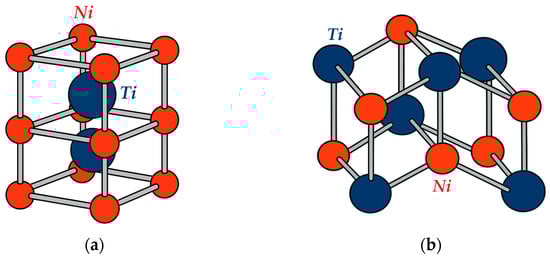
Figure 1.
Crystal structure of NiTi (a) austenitic phase B2 and (b) martensitic phase B19′.
SMAs exhibit two unique functional properties: the Shape Memory Effect (SME) and Superelasticity (SE), the latter often referred to as Pseudoelasticity (PE).
The Shape Memory Effect occurs during temperature changes, during which the alloy undergoes sequential phase transformations. Upon cooling, austenite transforms first into twinned martensite and subsequently into detwinned martensite. When heated, the material reverts to the austenitic state. This thermally driven transformation cycle repeats each time the alloy is cooled and reheated. Superelasticity, in contrast, manifests under isothermal conditions when the material temperature is equal to or exceeds the austenite finish temperature. Under these conditions, the alloy remains in a stable austenitic phase and transforms into detwinned martensite upon application of mechanical loading. Upon unloading, the structure returns to the austenitic state, fully recovering its original shape. This superelastic thermomechanical cycle begins at elevated temperatures in a fully austenitic state, proceeds through the formation of stable detwinned martensite under loading, and concludes with complete reversion to austenite upon unloading.
Owing to their ability to undergo reversible phase transformations, SMAs can recover their original shape in response to changes in temperature or applied mechanical loading. This unique mechanism is governed by microstructural rearrangements and the interplay between the material’s mechanical and functional properties. As a result of the reversible transformations occurring during the superelastic cycle, a hysteresis loop appears in the stress–strain space, the area of which corresponds to the energy dissipated by the material during transitions between austenite and martensite (Figure 2).
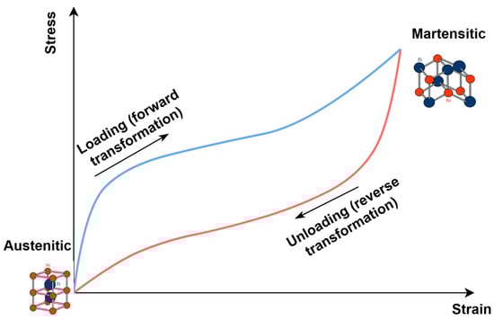
Figure 2.
Hysteresis loop of one SMA loading and unloading cycle.
The presence of energy dissipation reflects the alloy’s ability to convert part of the mechanical energy into heat during the austenite–martensite transformation. This behavior characterizes the material’s damping capacity and its superelastic response. Owing to these properties, shape memory alloys are highly effective for vibration suppression and operation under dynamic loading conditions. The dimensions of the hysteresis loop depend on the alloy’s chemical composition, thermal treatment, and external loading conditions.
The main advantages of SMA in actuators and sensors are their simple design and high degree of miniaturization [15]. Traditionally, actuators and sensors are based on elements made of functional materials (bimetallic plates, piezoelectric elements, etc.) capable of converting electrical, thermal, and magnetic energy into mechanical energy. Compared to these types of materials, SMAs offer lower actuator response times but significantly higher specific power output. They can also serve as both a control system and an actuator [16]. These actuators and sensors can operate independently of complex drives and mechanical systems, thereby reducing the overall weight and size of the devices.
The application of machine learning methods spans a wide range of research domains, including materials science [17,18,19,20,21,22,23], medicine [24,25,26,27,28,29], finance [30,31,32,33,34], engineering [35,36,37,38,39], and information technology [40,41,42,43,44]. There are known studies that deal with neural network modeling of the stress–strain state of materials with shape memory and structures made from them, which enable a careful consideration of their features and properties, ensuring the stability of operational characteristics in the presence of instability in macro- and microstructural parameters. Studying the obtained patterns can facilitate the analysis of the correlation between SMA microstructure and hysteresis behavior [45,46].
Due to their ability to process large datasets and identify complex nonlinear relationships, machine learning techniques enable the effective prediction of system and material behavior under diverse operating conditions. A considerable research effort has focused on modeling the properties of shape memory alloys using machine learning algorithms. Numerous studies confirmed the effectiveness of such approaches for predicting key SMA characteristics. The work in [47], for example, presents a comprehensive review of artificial neural network applications for modeling SMA properties, covering various neural network architectures and their performance in reproducing SMA behavior. In [48,49], a universal approach for predicting the martensitic transformation temperature in SMAs using machine learning techniques is proposed.
The authors derive an empirical formula for the martensitic transformation temperature, demonstrating strong generalizability across various SMA types. In [50], the feasibility of predicting the loading frequency of SMAs from experimental data using different machine learning methods is investigated. The study specifically shows that a multilayer perceptron (MLP) neural network achieves the highest classification accuracy. Predicting the loading frequency from known input parameters (such as stress, strain, and cycle number) allows researchers to determine the frequency at which the material dissipates a given amount of energy, which is essential for analyzing the functional behavior of SMAs. The study [51] employs machine learning methods to expedite the design of NiTi alloys with enhanced elastocaloric effects, which is promising for solid-state cooling. Nine new alloys were discovered during the learning process. The model showed high interpretability and efficiency. In article [52], a machine learning method is proposed for identifying the thermodynamic parameters of superelastic SMAs, which considers the dependence on the deformation rate. In study [53], machine learning models were developed to predict the mechanical properties of nickel-free titanium shape memory alloys. The research focused on forecasting the ultimate tensile strength (UTS) and elongation (EL). The Gradient Boosting Regression model demonstrated the highest accuracy for predicting EL, whereas the prediction of UTS proved to be less accurate. In [54], an LSTM-based model was developed to predict the rotational angle of a pulley in an SMA-wire-driven actuator, taking into account the hysteresis behavior of the alloy. In [55], an interpretable piecewise-linear regression model was developed and experimentally validated to identify the ranges of chemical and physical properties that lead to either B19 or B19′ transformation, as well as to predict a parameter derived from the chemical characteristics of the alloy composition. In study [56], a machine learning approach was employed to identify NiTiHf alloys suitable for actuator applications in space environments. The K-nearest neighbors model achieved the highest accuracy, enabling effective prediction of phase transformation temperatures. In [57], the authors demonstrated the effectiveness of statistical learning for predicting the martensitic transformation temperature of SMAs using three descriptors related to chemical bonding and atomic radii of the alloying elements. This approach accelerated the discovery of alloys with targeted transformation temperatures. In study [58], the behavior of NiTi SMAs was analyzed using a neural-network-based modeling approach, where the model predicted strain as a function of temperature. In [59], a platform was introduced for discovering new SMA compositions exhibiting narrow temperature hysteresis loops under applied loading. The work in [60] examined the use of a deep neural network to predict the outcomes of electrochemical processing of NiTi SMA. The model outperformed traditional approaches, demonstrating lower RMSE values and higher predictive accuracy. In a study [61], a neural network model was proposed to predict temperature and displacement in SMA-based actuators, eliminating the need for bulky position sensors.
One of the key limitations of studies that employ machine learning to predict SMA properties is the insufficient volume of experimental data. The limited availability of high-quality and representative datasets hinders effective model training, reducing predictive accuracy—particularly when modeling complex nonlinear behaviors. In particular, constructing models capable of accurately reproducing SMA behavior under repeated cyclic loading and unloading requires experimental data that capture a wide range of loading cycles and the progressive structural changes occurring with each subsequent cycle. This need becomes especially critical for accurately representing hysteresis loops under multiple cycles and varying loading frequencies. A review of the scientific literature on machine learning applications for SMA property prediction reveals a significant lack of studies focused on modeling hysteresis behavior under repeated cyclic loading. Predicting deformation under such conditions is essential, as it allows for estimating the amount of energy dissipated during phase transformations between martensite and austenite—a key parameter for many practical SMA applications.
The aim of this study is to develop and evaluate machine learning models for predicting the hysteresis behavior of SMAs, as well as to ensure the interpretability of these models through the application of Explainable Artificial Intelligence (XAI) techniques. The work focuses on improving strain-prediction accuracy and reducing forecasting errors. The integration of XAI enables the analysis of how individual input parameters contribute to the model’s predictions, thereby enhancing model transparency and supporting the physical validity of the results with respect to the underlying phase-transformation mechanisms in SMAs.
2. Materials and Methods
2.1. Data Collection and Preparation
The experimental data were obtained from low-cycle fatigue tests of a NiTi shape memory alloy wire with a diameter of 1.5 mm and a length of 210 mm. The wire was supplied by Wuxi Xin Xin Glai Steel Trade Co., Ltd. (Wuxi, China). The chemical composition of the material was 55.78% Ni and 44.12% Ti, with a total impurity content of 0.1% (Table 1).

Table 1.
Chemical composition of nitinol (%).
The Young’s modulus of nitinol in the austenitic state was EA = 52.7 GPa [62]. The onset of the forward austenite-to-martensite transformation occurred at a stress of σAM = 338 MPa. The tests were carried out in air at a temperature of 24 ± 1 °C using an STM-100 servo-hydraulic testing machine (Figure 3a) in stress-controlled mode, in accordance with ASTM F2516-14 [63]. Uniaxial tensile fatigue tests were performed under sinusoidal cyclic loading with a stress ratio of 0.1. During testing, the applied force, actuator displacement, and wire elongation were recorded. Experiments were conducted at various loading frequencies (f = 0.1, 0.3, 0.5, 1, 3, 5, and 10 Hz) [64]. Elongation was measured using a Bi-06-308 extensometer (Figure 3b) manufactured by Bangalore Integrated System Solutions (BISS), while displacement was recorded using a Bi-02-313 inductive displacement sensor (Figure 3c).
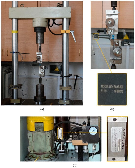
Figure 3.
The machine for the experiment: (a) general view of the STM-100; (b) test sample fixed in the grippers and Bi-06-308 sensor; (c) Bi-02-313 sensor.
The relative measurement error of the instruments, as indicated by their calibration certificates, did not exceed 0.1%. Stress σ (MPa) and strain ε (%) were determined from the recorded force–elongation data using the Test Builder software, version 5.3. At least three specimens were tested for each loading frequency. Hysteresis loops were saved for every cycle, which enabled the calculation of instantaneous stress, strain, and the dissipated energy Wdis, defined as the area enclosed by the loading–unloading loop. In this study, experimentally obtained data from 100 to 250 loading–unloading cycles of the SMA material were used for all seven loading frequencies: 0.1, 0.3, 0.5, 1, 3, 5, and 10 Hz.
2.2. Experimental Dataset Description and Correlation Analysis
The experimental dataset consisted of the applied stress σ (MPa), the loading cycle number N, the material strain ε (%), an indicator of loading or unloading, and the loading frequency f (Hz). The number of elements in the dataset for each of the seven frequencies is shown in Table 2.
Table 2.
Distribution of the number of elements in the dataset by cyclic load frequencies.
During the preliminary data processing, the dataset was first examined for abnormal values of Stress and Strain that could distort the statistical characteristics or adversely affect model training. To accomplish this, three independent criteria were applied sequentially.
First, the ±3sigma rule, also known as the k-sigma test [65], was applied. For each numerical variable, the mean μ and standard deviation sigma were computed. Any observation in which at least one variable fell outside the interval μ ± 3sigma was considered a potential outlier. This approach relies on the assumption of a quasi-normal distribution. Under a normal distribution, more than 99.7% of all data points are expected to lie within three standard deviations from the mean; therefore, a violation of this boundary indicates atypical behavior in the data. Next, the interquartile range (IQR) method, using the classical multiplier of 1.5, was applied [66]. For each feature, the first (Q1) and third (Q3) quartiles were computed, followed by the calculation of the interquartile range IQR = Q3 − Q1. The inner bounds were then defined using the standard formulas Q1 − 1.5·IQR and Q3 + 1.5·IQR. Any observation that exceeded these limits in at least one variable was flagged as a potential outlier. This method does not rely on any distributional assumptions and is robust to isolated extreme values. To identify local anomalies, a rolling z-score method [67] with a window of 20 points (10 preceding and 10 following the current point) was applied. Within this window, the local mean μ and standard deviation sigma were computed, and the condition |z| > 3 was checked. This approach is capable of detecting short-term spikes or drops that may not affect the global statistics but still disrupt the local structure of the signal. Each criterion operated independently. All candidates for removal were combined, duplicates were eliminated, and the total number of unique suspicious rows was counted. As a result of applying three independent methods for detecting outliers, less than 0.1% of samples were removed from the dataset for each loading frequency, which has no effect on the statistical distribution of the data. Outlier detection at this stage enhanced both the stability and the generalization capability of the models.
A correlation analysis [68] was also performed to evaluate the linear relationships between the input features Stress, Cycle, and UpDown and the output variable Strain, determining the degree of their mutual dependence before constructing machine learning regression models.
Figure 4 shows the correlation matrix for load frequencies of 0.1, 1, and 10 Hz.
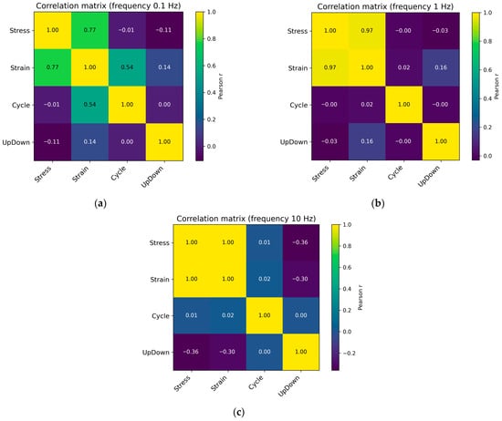
Figure 4.
Pearson correlation coefficient matrix for cyclic loading with a frequency of 0.1 Hz (a), 1 Hz (b), and 10 Hz (c).
Similar Pearson correlation matrices were generated for the remaining loading frequencies. As the loading frequency increases, a pronounced strengthening of the positive correlation between stress and strain is observed, accompanied by the disappearance of any meaningful correlation between strain and the cycle number. At the low frequency of 0.1 Hz, the Pearson correlation coefficient for the Stress–Strain pair is approximately 0.77, while Strain still exhibits a noticeable correlation with Cycle (≈0.54), reflecting the accumulation of residual deformation under slow, quasi-static loading conditions. Already at 0.3–0.5 Hz, the Stress–Strain correlation rises sharply to 0.93–0.94, while the Strain–Cycle relationship weakens. Under these conditions, the material has time to unload only partially, and strain becomes almost a direct function of the instantaneous stress rather than of the cycle history. A further increase in frequency (1–5 Hz) elevates the Stress–Strain correlation to 0.97–0.99, whereas all pairs involving Cycle remain close to zero. The mechanical response transitions into an almost elastic regime: the hysteresis loop narrows, and the accumulation effect disappears. At the highest frequency of 10 Hz, the Stress–Strain correlation reaches 1.00. Thus, as the frequency increases, the system evolves from a quasi-static, energy-dissipative regime to a high-rate regime approaching elastic–plastic behavior, in which Stress and Strain are fully correlated, and all other interactions diminish. The pseudoelastic effect becomes substantially diminished [69,70].
Multicollinearity among the input features is practically absent. The pairwise Pearson correlation coefficients in the correlation matrix fluctuate near zero, indicating that no feature pair exhibits a strong linear relationship. According to the commonly accepted threshold of ∣r∣ < 0.3, this confirms the absence of multicollinearity. To additionally verify multidimensional collinearity, the Variance Inflation Factor (VIF) values were computed [71]. All three input features have VIF ≈ 1, which indicates a complete absence of linear dependence between each feature and any linear combination of the remaining features. Although the machine learning models used in this study are not sensitive to multicollinearity, its absence confirms that no informational redundancy exists among the features and serves as an additional indicator of feature set quality.
As part of the data preparation process, the dataset was split into training and test subsets according to the group parameter Cycle, which denotes the loading cycle number of the material. Group-based splitting by Cycle ensured that data from different cycles did not mix between subsets, thereby preventing information leakage and providing an objective evaluation of the model. To construct the subsets, 80% of the cycles were assigned to the training set, while the remaining 20% were allocated to the test set. Thus, the model was trained on cycles within the range 100–250 but evaluated on an independent subset of cycles, ensuring a correct assessment of its generalization ability. Additionally, 10% of the training data was set aside for internal model validation during training. This split was also performed using the group-based principle with respect to the Cycle parameter, guaranteeing that validation cycles did not overlap with the training cycles. This approach enabled an objective assessment of the model’s generalization capability and ensured the reliability of comparisons between the predicted results and the experimental data.
2.3. Machine Learning Methods Used in the Study
The study employed neural networks of various architectures, including the Simple Recurrent Neural Network (SimpleRNN), Long Short-Term Memory (LSTM) network, and Gated Recurrent Unit (GRU) network.
2.4. Evaluation and Interpretation Methods
In this study, the model’s performance was evaluated using the mean absolute error (MAE), mean squared error (MSE), coefficient of determination (R2), and mean absolute percentage error (MAPE) [72].
MAE represents the average magnitude of the absolute deviations between the predicted and actual values, allowing one to assess how much the predictions differ from the true values on average. The MAE metric was computed using the following formula:
where is the true value of material strain in the test dataset, is the predicted value of material strain in the test dataset, and n is the size of the test dataset.
MSE provides an assessment of the magnitude of the squared error, emphasizing larger deviations because the quadratic function substantially amplifies the impact of large errors. The metric was calculated using the following formula:
MAPE reflects the average percentage deviation of the predicted values from the actual values, making it convenient for interpreting the relative accuracy of the predictions. The metric was calculated using the following formula:
The coefficient of determination R2 indicates how well the model explains the variance of the actual values in the test dataset. It was computed using the following formula:
where is the mean value of true material strains in the test dataset.
In this study, the machine learning models were interpreted using the Integrated Gradient (IG) method [73,74], which belongs to the class of Explainable Artificial Intelligence (XAI) techniques. Its application made it possible not only to quantitatively assess the contribution of individual features to the model’s decision-making process but also to enhance the transparency and credibility of the obtained results. The Integrated Gradients method computes the contribution of each feature to the model’s prediction by integrating the gradients of the output function along a straight-line path between a baseline (neutral) input and the actual input vector.
Let F(x) be a differentiable model (e.g., a neural network) that maps the input feature vector x = (x1, x2, …. xn) to a scalar prediction. Then, the contribution (integrated gradient) of the i-th feature is defined as:
where x′ = (x1′, x2′, …, xn′) is the baseline (neutral) input vector, for which the model output F(x′) is typically close to zero or otherwise non-informative, α ∈ [0, 1] is the parameter that traces the path from the baseline input to the actual example, and denotes the partial derivative (gradient) of the output function with respect to the i-th feature.
The resulting integrated gradients provide a quantitative measure of the contribution of each feature to the model’s output. The sum of all feature contributions approximates the difference between the predicted value and the baseline output:
The method is based on the axioms of Sensitivity and Implementation Invariance, which ensure its reliability and theoretical soundness [73]. This approach enables the evaluation of the influence of each feature on the model output while maintaining mathematical consistency with the model itself.
In our study, the IG method was applied to interpret neural network models (RNN, LSTM, GRU), all of which are differentiable architectures. This allowed us to analyze how variations in the input features affect the predicted output and to identify which parameters have the greatest influence on the model’s decisions. Visualization of the resulting feature contributions enabled the identification of the most significant factors and revealed hidden patterns that were not apparent from metric-based evaluation alone.
Additionally, several visualization tools were employed during the model evaluation process to perform a qualitative assessment of how well the predicted values matched the experimental data. The actual vs. predicted plot enabled an examination of the degree of agreement between the predicted and true values. The residual plot illustrated the distribution of prediction errors (the differences between actual and predicted values) as a function of the test sample index. Constructed hysteresis loops allowed for a visual comparison of the shapes of the experimental and predicted stress–strain curves. These visualizations complemented numerical evaluation metrics, providing a deeper insight into the behavior and reliability of the models.
3. Results and Discussion
3.1. Results of Neural Networks
3.1.1. Architecture
In this study, recurrent neural networks—SimpleRNN, LSTM, and GRU—were employed. These models belong to the class of deep learning architectures capable of effectively capturing temporal dependencies in sequential data. The architectures were built using the TensorFlow/Keras framework [75] with automated hyperparameter selection based on the Hyperband algorithm, which provides an efficient search for optimal configurations in a wide model space. Each model contains an input layer corresponding to the number of input features (Stress, Cycle, and UpDown), four hidden recurrent LSTM layers with nonlinear tanh activation and full sequence return, and an output layer that generates a deformation prediction for each time step. As part of the hyperparameter optimization procedure, the number of neurons in the hidden recurrent layers was varied in the range 32–256 with a step size of 32. The number of hidden LSTM layers varied from one to four. For each recurrent layer, Dropout coefficients were automatically selected within the range of 0.1–0.5 with a step size of 0.1, allowing for the control of regularization and a reduction in the risk of overfitting.
To ensure stable convergence of the learning process in all architectures, the Adam optimizer with exponential learning rate decay was used, implemented through the ExponentialDecay mechanism, where the initial value of the learning rate parameter was 0.001 or 0.0001, after which an exponential decrease in the learning rate with a coefficient of 0.96 was applied every 1000 steps. The final value was fixed at initial_lr = 0.001 for the final models. This approach ensured an adaptive reduction in the learning rate during training, contributing to a gradual approach to the minimum loss function without sharp fluctuations. In addition, an EarlyStopping mechanism with a patience parameter of 150 was used, which automatically stops training when the validation error stabilizes and restores the weights corresponding to the best model state. The combination of automated hyperparameter selection, adaptive optimization, and early stopping made it possible to increase the stability of the learning process, accelerate convergence, and ensure the high generalization ability of recurrent neural networks. The final configuration of each model was determined by the minimum value of the MSE loss function on the validation sample.
The architectural parameters and the results of the automated tuning procedure are summarized in Table 3, Table 4 and Table 5.
Table 3.
Main hyperparameters of the SimpleRNN-based neural network models.
Table 4.
Main hyperparameters of the LSTM-based neural network models.
Table 5.
Main hyperparameters of the GRU-based neural network models.
3.1.2. Performance Evaluation
Model performance was evaluated using standard regression metrics, including MSE, MAE, R2, and MAPE. The results for the three architectures and seven loading frequencies are summarized in Table 6.
Table 6.
Accuracy metrics of the SimpleRNN, LSTM, and GRU models for different loading frequencies.
Analysis of the results presented in Table 6 shows that all recurrent architectures achieved high accuracy on the test data. For all models, the coefficient of determination exceeds R2 = 0.999, indicating an almost perfect agreement between the experimental and predicted strain values.
To visually assess the quality of the predictions, actual versus predicted plots were constructed to illustrate the relationship between the experimental and computed strain values. This approach provides an intuitive means of verifying how well the model aligns with the real data. Points located along the line y = x indicate high prediction accuracy and the absence of systematic bias between the predicted and actual values (Figure 5).
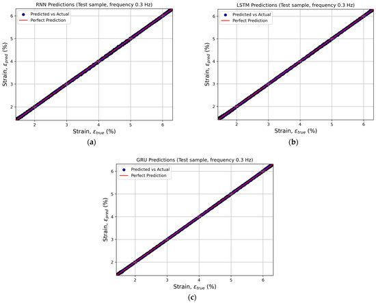
Figure 5.
Comparison of the actual and predicted strain values at a loading frequency of 0.3 Hz for recurrent neural networks: (a) SimpleRNN, (b) LSTM, and (c) GRU.
Similar plots were generated for the remaining loading frequencies. The results showed that, for all frequencies, the data points cluster tightly around the bisector of the first coordinate angle.
Additionally, to assess the quality of prediction, residual plots were constructed, reflecting the distribution of differences between actual and predicted deformation values as a function of the measurement number (sample) in the test subsample. This analysis enables the detection of potential systematic errors, local deviations, or hidden trends that may not be apparent from other evaluation metrics (Figure 6).
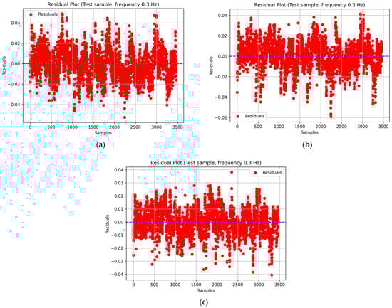
Figure 6.
Residual plots for SimpleRNN (a), LSTM (b), and GRU (c) models at a loading frequency of 0.3 Hz.
Similar plots were generated for the remaining loading frequencies. For all models, the residuals exhibit a random distribution with no visible trends or systematic deviations from the zero line, indicating the absence of systematic errors and demonstrating proper model generalization. The amplitude of residual fluctuations does not exceed ±0.05, which confirms the high stability of the predictions and the well-balanced training of the recurrent neural networks.
3.1.3. Verification of Generalization Ability
To evaluate the ability of the developed recurrent neural networks to generalize beyond the training and test ranges, independent testing was performed on loading cycles that were not included in either subset—specifically, cycles 251, 260, 300, 350, 400, 450, and 500. This testing aimed to assess the extrapolation capability of the models, that is, their ability to predict the hysteresis behavior of the alloy as fatigue effects continue to accumulate.
The values of MSE, MAE, R2, and MAPE for the three architectures and seven loading frequencies are presented in Appendix A.
The results obtained indicate high prediction accuracy in the area closest to the training sample (251–300 cycles) and a gradual increase in errors with increasing cycle number. The increase in errors during extrapolation to distant cycles (>300) is not a disadvantage of the neural network architecture, but rather a consequence of physically induced material degradation associated with the accumulation of fatigue effects that exceed the information available to the model at the training stage.
At a frequency of 0.1 Hz (Table A1), all models accurately reproduced the hysteresis loops up to cycle 300. Beginning with cycle 350, the accuracy of the SimpleRNN and GRU architectures decreased sharply, whereas the LSTM network maintained acceptable accuracy (R2 = 0.9244, MAE ≈ 0.1672 at cycle 400) and demonstrated the strongest extrapolation capability, remaining reliable up to cycle 500. The deformation processes occur more slowly at a frequency of 0.1 Hz, which causes the most pronounced hysteresis behavior of the material. Hysteresis, by its nature, is a process with ‘memory,’ in which the current state of the system is determined by the entire previous load history. With an increase in the number of cycles (after approximately 350), the accumulated error in models that do not work effectively with long-term dependencies becomes critical. The SimpleRNN architecture has the simplest structure and is most susceptible to the vanishing gradient problem, resulting in the loss of information from the early stages of loading in long sequences. Although GRU manages information flows more efficiently using update gate and reset gate mechanisms, its simplified structure with a combined hidden state and memory limits its ability to predict long-term material degradation. In contrast, LSTM is specifically designed to model long-term dependencies through the presence of a separate cell state, which ensures stable information transfer over time. The forget gate mechanism enables the selective rejection of irrelevant data while preserving key features of load evolution over hundreds of cycles, which is crucial for accurately predicting hysteresis loops under low-frequency loading.
At a frequency of 0.3 Hz (Table A2), all architectures preserved high prediction accuracy across the entire range. The LSTM model exhibited the lowest errors and proved to be the optimal architecture for this frequency. At a frequency of 0.5 Hz (Table A3), the prediction accuracy remained consistently high up to cycle 450. At cycle 500, the LSTM model demonstrated the best performance (R2 = 0.9912, MAE = 0.0572). Thus, LSTM is the most effective architecture for this frequency. At 1 Hz (Table A4), all models showed excellent agreement with the experimental data up to cycle 400. With further increases in cycle number, the accuracy decreased slightly; however, LSTM maintained the highest performance (R2 = 0.9976, MAE = 0.0282 at cycle 500). At a frequency of 3 Hz (Table A5), all models exhibited high prediction quality; however, LSTM produced the lowest errors and the most stable convergence (R2 = 0.9867, MAE = 0.0629 at cycle 500). The GRU model exhibited similar accuracy but showed slightly greater variability in error at higher cycle numbers. Therefore, LSTM is the most suitable architecture for a 3 Hz signal. For the 5 Hz frequency (Table A6), the GRU model achieved the best performance (R2 = 0.9805, MAE = 0.0614 at cycle 500). At the highest frequency of 10 Hz (Table A7), all models maintained high accuracy within the first extrapolated cycles (251–350), although accuracy decreased for more distant cycles. The LSTM model demonstrated the most stable performance (R2 = 0.9979, MAE = 0.0153, MAPE = 0.8% at cycle 500).
Summarizing the results across all frequencies, the following conclusions can be drawn:
- LSTM demonstrated the highest stability and extrapolation accuracy for frequencies of 0.1–3 Hz and 10 Hz;
- GRU proved to be the optimal architecture for 5 Hz;
- SimpleRNN provides acceptable accuracy only within the training range but loses consistency during long-range extrapolation (beyond approximately 350 cycles).
Thus, the LSTM and GRU models demonstrated strong generalization capability and robust extrapolation performance in predicting the hysteresis behavior of SMAs under cyclic loading, making them suitable for long-term forecasting applications.
3.1.4. Comparison of Experimental and Predicted Hysteresis Loops
For all loading frequencies and for all recurrent neural network architectures, experimental and predicted hysteresis loops were constructed for cycles 251, 260, 300, 350, 400, 450, 500, and 600. This graphical representation enabled the visual comparison of the predicted loop shapes with the experimental data, allowing for an assessment of the models’ ability to accurately reproduce phase transitions and fatigue-accumulation effects. Across all frequencies, a high degree of agreement was observed between the predicted and experimental curves, further confirming the physical credibility of the obtained predictions.
Figure 7 and Figure 8 present an example of the comparison between the experimental and predicted hysteresis loops generated by the LSTM model for cycles 251, 260, 300, 350, 400, 450, 500, and 600 at a loading frequency of 0.3 Hz. Within the range of cycles 251–300, the predicted and experimental curves almost perfectly overlap, demonstrating the model’s high accuracy in reproducing the material’s hysteresis behavior (Figure 7).
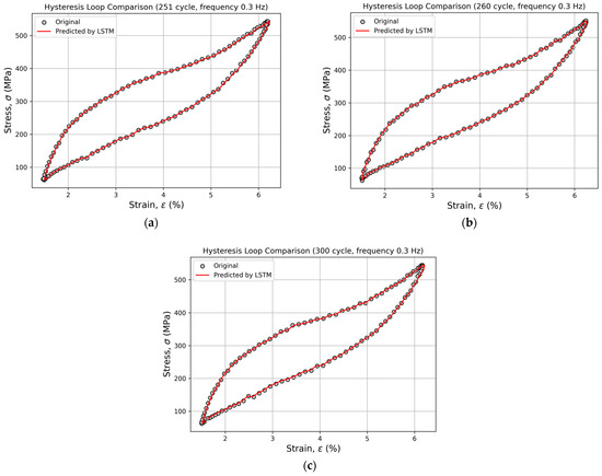
Figure 7.
Comparison of experimental and predicted hysteresis loops for cycles 251 (a), 260 (b), and 300 (c) at a loading frequency of 0.3 Hz, obtained using the LSTM model.
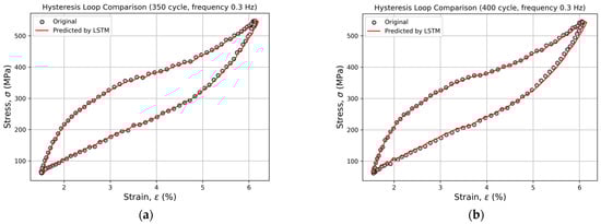
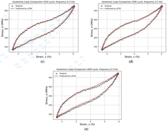
Figure 8.
Comparison of experimental and predicted hysteresis loops for cycles 350 (a), 400 (b), 450 (c), 500 (d), and 600 (e) at a loading frequency of 0.3 Hz, obtained using the LSTM model.
Starting from cycle 350, slight deviations become noticeable in the upper portion of the loop (Figure 8).
Even at cycle 600, the model adequately reproduces the phase transitions and the overall loop shape, demonstrating its robust extrapolation capability and strong physical consistency.
3.2. Interpretation of Neural Network Results
In this study, the Integrated Gradients method was applied to analyze the SimpleRNN, LSTM, and GRU models. The method made it possible to determine which input parameters (stress (σ), loading cycle number (N), and the loading–unloading indicator (UpDown)) have the greatest influence on the predicted strain (ε).
The analysis was performed at both the local level (for individual loading cycles) and the global level (for the entire dataset). To generalize the results across the full dataset, the mean absolute attribution value was used, representing the average magnitude of the influence of each feature on the model output (attribution). This metric reflects the average contribution of each feature to a single prediction, eliminating dependence on the number of points per cycle or the dataset size. Such an approach ensures a correct comparison of global feature importance across different loading frequencies and models and aligns with standard practices for evaluating global attributions in contemporary XAI research. For an individual cycle, the total importance was computed as the sum of the absolute attribution values for each feature within that cycle. This metric reflects the integrated influence of a feature on the predicted strain across the entire loading–unloading cycle. The use of total importance is particularly appropriate for analyzing the evolution of the influence of physical parameters over time, i.e., as the number of loading–unloading cycles increases.
Figure 9 presents the global distribution of feature importance for the LSTM model, obtained using the IG method at a loading frequency of 0.3 Hz
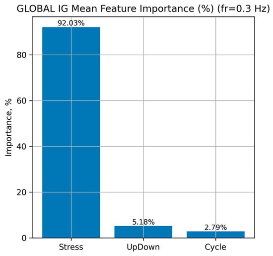
Figure 9.
Global distribution of input-feature importance for the LSTM neural network at a loading frequency of 0.3 Hz.
The results show that the dominant factor determining the predicted Strain is Stress, which accounts for approximately 92.0% of the overall mean importance. The features UpDown (approximately 5.2%) and Cycle (approximately 2.8%) contribute substantially less, indicating their secondary influence compared with Stress.
Figure 10 presents the distribution of local feature importance for individual loading cycles (251, 300, 400, 500, and 600) at a frequency of 0.3 Hz for the LSTM neural network.
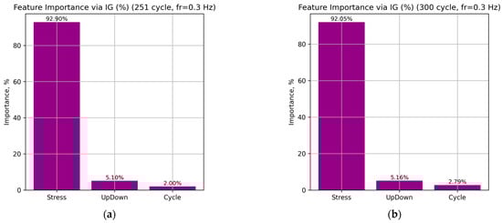
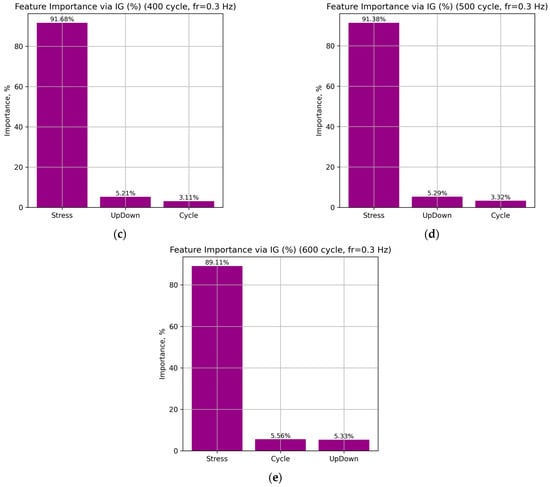
Figure 10.
Distribution of the total importance of input features for the LSTM neural network at a frequency of 0.3 Hz: cycles 251 (a), 300 (b), 400 (c), 500 (d), and 600 (e).
According to the obtained results, the Stress feature dominates in all cases, accounting for 92.90–89.11% of the total attribution sum, which indicates its leading role in determining the predicted strain. The UpDown feature provides a stable but secondary contribution (5.10–5.33%), associated with transitions between the loading and unloading phases. Meanwhile, the influence of the Cycle parameter gradually increases from 2.00% to 5.56% as the number of cycles increases, indicating that the model correctly captures the accumulation of fatigue effects in the material.
This distribution of attributions is consistent with the physical nature of deformation processes in NiTi SMA. Variations in Stress directly govern the phase transitions between martensite and austenite. The relatively constant contribution of UpDown reflects the model’s consistent reproduction of hysteresis behavior during loading and unloading. The Cycle parameter represents the long-term fatigue accumulation effect.
4. Conclusions
This work presents an approach to predicting the hysteresis behavior of NiTi shape memory alloys which integrates recurrent neural networks (SimpleRNN, LSTM, GRU) with XAI-based interpretability methods. The experimental dataset was constructed from loading–unloading cycles at seven loading frequencies (0.1, 0.3, 0.5, 1, 3, 5, and 10 Hz) between 100 and 250 cycles. Generalization capability was evaluated on independent cycles 251, 260, 300, 350, 400, 450, and 500. The data were split according to the Cycle group parameter, which prevents information leakage between subsets and ensures an objective evaluation of model performance.
The results demonstrate high modeling accuracy across the entire frequency range. On the test subsets, all architectures achieved an R2 value greater than 0.999, with very low MAE, MSE, and MAPE values. The residuals exhibit a random distribution without systematic trends, confirming proper model training and strong agreement between predictions and experimental measurements. Extrapolation tests showed that high accuracy is retained for cycles 251–300, with errors gradually increasing for later cycles due to the accumulation of fatigue effects. Among the architectures, the LSTM network showed the highest accuracy and strongest extrapolation capability for frequencies ranging from 0.1 to 3 Hz and 10 Hz, whereas the GRU model performed best at 5 Hz. Visual comparison of the experimental and predicted hysteresis loops confirmed that the phase transitions between austenite and martensite were accurately reproduced, even at distant cycles.
Model explainability using Integrated Gradients revealed that Stress is the dominant factor determining the predicted strain. The UpDown feature has a stable but secondary contribution associated with the transition between loading and unloading phases. The influence of the Cycle parameter increases gradually with cycle number, indicating that the model correctly captures the progressive accumulation of fatigue effects in the material. These interpretability results enhance trust in the predictions and support the physical validity of the models.
Future work will focus on integrating Temporal Convolutional Networks (TCNs) as an alternative architecture. The application of TCNs represents a promising direction for further enhancing the model’s extrapolation capability.
Author Contributions
Conceptualization, D.T. and O.Y.; methodology, D.T. and O.Y.; software, D.T.; validation, D.T., O.Y. and I.D.; formal analysis, P.M. and N.L.; investigation, D.T. and I.D.; resources, N.L.; data curation, D.T. and N.L.; writing—original draft preparation, D.T. and O.Y.; writing—review and editing, D.T., O.Y. and I.D.; visualization, D.T.; supervision, P.M.; project administration, P.M.; funding acquisition, P.M. All authors have read and agreed to the published version of the manuscript.
Funding
This research received no external funding.
Data Availability Statement
The raw data supporting the conclusions of this article will be made available by the authors on request.
Conflicts of Interest
The authors declare no conflicts of interest.
Appendix A
Table A1.
Accuracy metrics of the SimpleRNN, LSTM, and GRU models at a loading frequency of 0.1 Hz.
Table A1.
Accuracy metrics of the SimpleRNN, LSTM, and GRU models at a loading frequency of 0.1 Hz.
| Model | Cycle | MSE | MAE | R2 | MAPE |
|---|---|---|---|---|---|
| SimpleRNN | 251 | 0.0011 | 0.0266 | 0.9990 | 0.0029 |
| 260 | 0.0018 | 0.0324 | 0.9982 | 0.0036 | |
| 300 | 0.0562 | 0.1823 | 0.9343 | 0.0204 | |
| 350 | 0.3457 | 0.4423 | 0.5341 | 0.0496 | |
| 400 | 0.6182 | 0.6096 | 0.1619 | 0.0685 | |
| 450 | 0.6629 | 0.6303 | 0.0053 | 0.0699 | |
| 500 | 0.7200 | 0.6597 | −0.1014 | 0.0731 | |
| LSTM | 251 | 0.0006 | 0.0223 | 0.9994 | 0.0024 |
| 260 | 0.0007 | 0.0224 | 0.9993 | 0.0024 | |
| 300 | 0.0048 | 0.0593 | 0.9944 | 0.0063 | |
| 350 | 0.0162 | 0.0966 | 0.9782 | 0.0105 | |
| 400 | 0.0557 | 0.1672 | 0.9244 | 0.0188 | |
| 450 | 0.0775 | 0.1966 | 0.8836 | 0.0219 | |
| 500 | 0.1329 | 0.2663 | 0.7966 | 0.0296 | |
| GRU | 251 | 0.0008 | 0.0242 | 0.9993 | 0.0026 |
| 260 | 0.0035 | 0.0535 | 0.9967 | 0.0056 | |
| 300 | 0.0628 | 0.2319 | 0.9266 | 0.0238 | |
| 350 | 0.2212 | 0.4571 | 0.7019 | 0.0474 | |
| 400 | 0.4344 | 0.6508 | 0.4110 | 0.0682 | |
| 450 | 0.6044 | 0.7665 | 0.0930 | 0.0797 | |
| 500 | 0.7636 | 0.8510 | -0.1681 | 0.0886 |
Table A2.
Accuracy metrics of the SimpleRNN, LSTM, and GRU models at a loading frequency of 0.3 Hz.
Table A2.
Accuracy metrics of the SimpleRNN, LSTM, and GRU models at a loading frequency of 0.3 Hz.
| Model | Cycle | MSE | MAE | R2 | MAPE |
|---|---|---|---|---|---|
| SimpleRNN | 251 | 0.0005 | 0.0180 | 0.9998 | 0.0049 |
| 260 | 0.0001 | 0.0097 | 0.9999 | 0.0030 | |
| 300 | 0.0007 | 0.0207 | 0.9997 | 0.0056 | |
| 350 | 0.0044 | 0.0555 | 0.9983 | 0.0146 | |
| 400 | 0.0080 | 0.0738 | 0.9968 | 0.0180 | |
| 450 | 0.0089 | 0.0795 | 0.9964 | 0.0197 | |
| 500 | 0.0141 | 0.1016 | 0.9941 | 0.0260 | |
| LSTM | 251 | 0.0003 | 0.0138 | 0.9999 | 0.0043 |
| 260 | 0.0008 | 0.0077 | 0.9999 | 0.0025 | |
| 300 | 0.0003 | 0.0153 | 0.9999 | 0.0052 | |
| 350 | 0.0010 | 0.0278 | 0.9996 | 0.0078 | |
| 400 | 0.0019 | 0.0368 | 0.9992 | 0.0096 | |
| 450 | 0.0018 | 0.0366 | 0.9992 | 0.0113 | |
| 500 | 0.0022 | 0.0430 | 0.9990 | 0.0145 | |
| 600 | 0.0122 | 0.0838 | 0.9946 | 0.0241 | |
| GRU | 251 | 0.0001 | 0.0091 | 0.9999 | 0.0024 |
| 260 | 0.0009 | 0.0064 | 0.9999 | 0.0018 | |
| 300 | 0.0004 | 0.0152 | 0.9998 | 0.0045 | |
| 350 | 0.0010 | 0.0254 | 0.9996 | 0.0060 | |
| 400 | 0.0023 | 0.0405 | 0.9990 | 0.0105 | |
| 450 | 0.0015 | 0.0327 | 0.9993 | 0.0106 | |
| 500 | 0.0028 | 0.0467 | 0.9988 | 0.0151 |
Table A3.
Accuracy metrics of the SimpleRNN, LSTM, and GRU models at a loading frequency of 0.5 Hz.
Table A3.
Accuracy metrics of the SimpleRNN, LSTM, and GRU models at a loading frequency of 0.5 Hz.
| Model | Cycle | MSE | MAE | R2 | MAPE |
|---|---|---|---|---|---|
| SimpleRNN | 251 | 0.0001 | 0.0130 | 0.9996 | 0.0041 |
| 260 | 0.0002 | 0.0075 | 0.9998 | 0.0027 | |
| 300 | 0.0003 | 0.0132 | 0.9994 | 0.0045 | |
| 350 | 0.0003 | 0.0152 | 0.9992 | 0.0049 | |
| 400 | 0.0006 | 0.0204 | 0.9987 | 0.0067 | |
| 450 | 0.0012 | 0.0305 | 0.9973 | 0.0096 | |
| 500 | 0.0059 | 0.0682 | 0.9874 | 0.0200 | |
| LSTM | 251 | 0.0001 | 0.0074 | 0.9999 | 0.0025 |
| 260 | 0.0001 | 0.0097 | 0.9998 | 0.0032 | |
| 300 | 0.0002 | 0.0118 | 0.9994 | 0.0042 | |
| 350 | 0.0009 | 0.0271 | 0.9980 | 0.0086 | |
| 400 | 0.0008 | 0.0246 | 0.9980 | 0.0086 | |
| 450 | 0.0015 | 0.0337 | 0.9966 | 0.0112 | |
| 500 | 0.0041 | 0.0572 | 0.9912 | 0.0180 | |
| GRU | 251 | 0.0001 | 0.0073 | 0.9998 | 0.0028 |
| 260 | 0.0003 | 0.0147 | 0.9995 | 0.0045 | |
| 300 | 0.0007 | 0.0234 | 0.9986 | 0.0076 | |
| 350 | 0.0012 | 0.0309 | 0.9974 | 0.0103 | |
| 400 | 0.0023 | 0.0419 | 0.9949 | 0.0124 | |
| 450 | 0.0040 | 0.0567 | 0.9911 | 0.0170 | |
| 500 | 0.0094 | 0.0864 | 0.9797 | 0.0250 |
Table A4.
Accuracy metrics of the SimpleRNN, LSTM, and GRU models at a loading frequency of 1 Hz.
Table A4.
Accuracy metrics of the SimpleRNN, LSTM, and GRU models at a loading frequency of 1 Hz.
| Model | Cycle | MSE | MAE | R2 | MAPE |
|---|---|---|---|---|---|
| SimpleRNN | 251 | 0.0001 | 0.0094 | 0.9997 | 0.0037 |
| 260 | 0.0001 | 0.0117 | 0.9996 | 0.0047 | |
| 300 | 0.0005 | 0.0185 | 0.9989 | 0.0087 | |
| 350 | 0.0019 | 0.0354 | 0.9959 | 0.0166 | |
| 400 | 0.0041 | 0.0546 | 0.9916 | 0.0247 | |
| 450 | 0.0076 | 0.0783 | 0.9842 | 0.0337 | |
| 500 | 0.0125 | 0.1015 | 0.9735 | 0.0408 | |
| LSTM | 251 | 0.0001 | 0.0084 | 0.9998 | 0.0036 |
| 260 | 0.0001 | 0.0077 | 0.9998 | 0.0031 | |
| 300 | 0.0001 | 0.0081 | 0.9998 | 0.0034 | |
| 350 | 0.0003 | 0.0144 | 0.9993 | 0.0064 | |
| 400 | 0.0005 | 0.0198 | 0.9990 | 0.0083 | |
| 450 | 0.0008 | 0.0247 | 0.9983 | 0.0108 | |
| 500 | 0.0011 | 0.0282 | 0.9976 | 0.0121 | |
| GRU | 251 | 0.0001 | 0.0081 | 0.9998 | 0.0036 |
| 260 | 0.0001 | 0.0090 | 0.9997 | 0.0039 | |
| 300 | 0.0002 | 0.0121 | 0.9995 | 0.0056 | |
| 350 | 0.0008 | 0.0210 | 0.9984 | 0.0099 | |
| 400 | 0.0013 | 0.0250 | 0.9973 | 0.0123 | |
| 450 | 0.0023 | 0.0322 | 0.9953 | 0.0159 | |
| 500 | 0.0027 | 0.0368 | 0.9942 | 0.0177 |
Table A5.
Accuracy metrics of the SimpleRNN, LSTM, and GRU models at a loading frequency of 3 Hz.
Table A5.
Accuracy metrics of the SimpleRNN, LSTM, and GRU models at a loading frequency of 3 Hz.
| Model | Cycle | MSE | MAE | R2 | MAPE |
|---|---|---|---|---|---|
| SimpleRNN | 251 | 0.0001 | 0.0084 | 0.9997 | 0.0044 |
| 260 | 0.0001 | 0.0080 | 0.9997 | 0.0041 | |
| 300 | 0.0004 | 0.0155 | 0.9990 | 0.0069 | |
| 350 | 0.0015 | 0.0307 | 0.9967 | 0.0139 | |
| 400 | 0.0045 | 0.0516 | 0.9909 | 0.0221 | |
| 450 | 0.0083 | 0.0693 | 0.9835 | 0.0298 | |
| 500 | 0.0114 | 0.0827 | 0.9775 | 0.0367 | |
| LSTM | 251 | 0.0001 | 0.0054 | 0.9999 | 0.0030 |
| 260 | 0.0001 | 0.0076 | 0.9998 | 0.0036 | |
| 300 | 0.0002 | 0.0107 | 0.9994 | 0.0059 | |
| 350 | 0.0006 | 0.0171 | 0.9987 | 0.0084 | |
| 400 | 0.0025 | 0.0372 | 0.9949 | 0.0168 | |
| 450 | 0.0047 | 0.0506 | 0.9906 | 0.0223 | |
| 500 | 0.0067 | 0.0629 | 0.9867 | 0.0290 | |
| GRU | 251 | 0.0001 | 0.0054 | 0.9999 | 0.0027 |
| 260 | 0.0001 | 0.0043 | 0.9999 | 0.0019 | |
| 300 | 0.0002 | 0.0142 | 0.9994 | 0.0074 | |
| 350 | 0.0007 | 0.0232 | 0.9985 | 0.0119 | |
| 400 | 0.0028 | 0.0492 | 0.9943 | 0.0250 | |
| 450 | 0.0049 | 0.0645 | 0.9902 | 0.0329 | |
| 500 | 0.0070 | 0.0722 | 0.9862 | 0.0376 |
Table A6.
Accuracy metrics of the SimpleRNN, LSTM, and GRU models at a loading frequency of 5 Hz.
Table A6.
Accuracy metrics of the SimpleRNN, LSTM, and GRU models at a loading frequency of 5 Hz.
| Model | Cycle | MSE | MAE | R2 | MAPE |
|---|---|---|---|---|---|
| SimpleRNN | 251 | 0.0001 | 0.0061 | 0.9997 | 0.0033 |
| 260 | 0.0001 | 0.0105 | 0.9992 | 0.0055 | |
| 300 | 0.0056 | 0.0691 | 0.9797 | 0.0467 | |
| 350 | 0.0071 | 0.0731 | 0.9765 | 0.0488 | |
| 400 | 0.0106 | 0.0915 | 0.9679 | 0.0579 | |
| 450 | 0.0182 | 0.1125 | 0.9479 | 0.0602 | |
| 500 | 0.0329 | 0.1492 | 0.9111 | 0.0740 | |
| LSTM | 251 | 0.0001 | 0.0054 | 0.9998 | 0.0030 |
| 260 | 0.0001 | 0.0089 | 0.9995 | 0.0046 | |
| 300 | 0.0055 | 0.0699 | 0.9799 | 0.0470 | |
| 350 | 0.0082 | 0.0860 | 0.9730 | 0.0562 | |
| 400 | 0.0112 | 0.0962 | 0.9661 | 0.0642 | |
| 450 | 0.0117 | 0.0934 | 0.9664 | 0.0606 | |
| 500 | 0.0181 | 0.1137 | 0.9510 | 0.0739 | |
| GRU | 251 | 0.0001 | 0.0032 | 0.9999 | 0.0019 |
| 260 | 0.0002 | 0.0126 | 0.9991 | 0.0069 | |
| 300 | 0.0072 | 0.0815 | 0.9739 | 0.0535 | |
| 350 | 0.0063 | 0.0746 | 0.9792 | 0.0493 | |
| 400 | 0.0070 | 0.0729 | 0.9788 | 0.0481 | |
| 450 | 0.0057 | 0.0578 | 0.9835 | 0.0355 | |
| 500 | 0.0072 | 0.0614 | 0.9805 | 0.0367 |
Table A7.
Accuracy metrics of the SimpleRNN, LSTM, and GRU models at a loading frequency of 10 Hz.
Table A7.
Accuracy metrics of the SimpleRNN, LSTM, and GRU models at a loading frequency of 10 Hz.
| Model | Cycle | MSE | MAE | R2 | MAPE |
|---|---|---|---|---|---|
| SimpleRNN | 251 | 0.0001 | 0.0058 | 0.9995 | 0.0031 |
| 260 | 0.0001 | 0.0076 | 0.9991 | 0.0041 | |
| 300 | 0.0003 | 0.0137 | 0.9973 | 0.0069 | |
| 350 | 0.0002 | 0.0103 | 0.9987 | 0.0055 | |
| 400 | 0.0005 | 0.0185 | 0.9959 | 0.0089 | |
| 450 | 0.0006 | 0.0182 | 0.9951 | 0.0090 | |
| 500 | 0.0014 | 0.0335 | 0.9902 | 0.0181 | |
| LSTM | 251 | 0.0001 | 0.0056 | 0.9996 | 0.0029 |
| 260 | 0.0001 | 0.0041 | 0.9997 | 0.0022 | |
| 300 | 0.0001 | 0.0107 | 0.9984 | 0.0058 | |
| 350 | 0.0002 | 0.0120 | 0.9981 | 0.0061 | |
| 400 | 0.0001 | 0.0100 | 0.9988 | 0.0054 | |
| 450 | 0.0003 | 0.0159 | 0.9971 | 0.0083 | |
| 500 | 0.0003 | 0.0153 | 0.9979 | 0.0082 | |
| GRU | 251 | 0.0001 | 0.0055 | 0.9996 | 0.0030 |
| 260 | 0.0001 | 0.0053 | 0.9995 | 0.0029 | |
| 300 | 0.0003 | 0.0125 | 0.9974 | 0.0064 | |
| 350 | 0.0004 | 0.0149 | 0.9969 | 0.0083 | |
| 400 | 0.0016 | 0.0310 | 0.9874 | 0.0158 | |
| 450 | 0.0058 | 0.0576 | 0.9565 | 0.0298 | |
| 500 | 0.0099 | 0.0836 | 0.9302 | 0.0456 |
References
- Chaudhary, K.; Haribhakta, V.K.; Jadhav, P.V. A review of shape memory alloys in MEMS devices and biomedical applications. Mater. Today Proc. 2024; in press. [Google Scholar] [CrossRef]
- Abbas, A.; Hung, H.-Y.; Lin, P.-C.; Yang, K.-C.; Chen, M.-C.; Lin, H.-C.; Han, Y.-Y. Atomic layer deposited TiO2 films on an equiatomic NiTi shape memory alloy for biomedical applications. J. Alloys Compd. 2021, 886, 161282. [Google Scholar] [CrossRef]
- Sharma, K.; Srinivas, G. Flying smart: Smart materials used in aviation industry. Mater. Today Proc. 2020, 27, 244–250. [Google Scholar] [CrossRef]
- Künnecke, S.C.; Vasista, S.; Riemenschneider, J.; Keimer, R.; Kintscher, M. Review of Adaptive Shock Control Systems. Appl. Sci. 2021, 11, 817. [Google Scholar] [CrossRef]
- Bovesecchi, G.; Corasaniti, S.; Costanza, G.; Tata, M.E. A novel self-deployable solar sail system activated by shape memory alloys. Aerospace 2019, 6, 78. [Google Scholar] [CrossRef]
- Costanza, G.; Tata, M.E. Shape memory alloys for aerospace, recent developments, and new applications: A short review. Materials 2020, 13, 1856. [Google Scholar] [CrossRef]
- Niu, X.; Yao, X.; Dong, E. Design and control of bio-inspired joints for legged robots driven by shape memory alloy wires. Biomimetics 2025, 10, 378. [Google Scholar] [CrossRef] [PubMed]
- Sun, L.; Gu, H. Envelope morphology of an elephant trunk-like robot based on differential cable–sma spring actuation. Actuators 2025, 14, 100. [Google Scholar] [CrossRef]
- Schmelter, T.; Bade, L.; Kuhlenkötter, B. A two-finger gripper actuated by shape memory alloy for applications in automation technology with minimized installation space. Actuators 2024, 13, 425. [Google Scholar] [CrossRef]
- Wang, X.-Y.; Pei, Y.-C.; Yao, Z.-Y.; Wang, B.-H.; Wu, L. A multi-functional sensing unit of planar 3DOFs displacements and forces based on superelastic SMA wires. Sens. Actuators A Phys. 2024, 377, 115766. [Google Scholar] [CrossRef]
- Riccio, A.; Sellitto, A.; Ameduri, S.; Concilio, A.; Arena, M. Shape memory alloys (SMA) for automotive applications and challenges. In Shape Memory Alloy Engineering; Elsevier: Amsterdam, The Netherlands, 2021; pp. 785–808. [Google Scholar] [CrossRef]
- Turabimana, P.; Sohn, J.W.; Choi, S.-B. Design and control of a shape memory alloy-based idle air control actuator for a mid-size passenger vehicle application. Appl. Sci. 2024, 14, 4784. [Google Scholar] [CrossRef]
- Zhang, H.; Zhao, L.; Li, A.; Xu, S. Design and hysteretic performance analysis of a novel multi-layer self-centering damper with shape memory alloy. Buildings 2024, 14, 483. [Google Scholar] [CrossRef]
- Pereiro-Barceló, J.; Bonet, J.L.; Martínez-Jaén, B.; Cabañero-Escudero, B. Design recommendations for columns made of ultra-high-performance concrete and NiTi SMA bars. Buildings 2023, 13, 991. [Google Scholar] [CrossRef]
- Pruski, A.; Kihl, H. Shape Memory Alloy Hysteresis. Sens. Actuators A 1993, 36, 29–35. [Google Scholar] [CrossRef]
- Li, Y.; Lin, J.; Zhao, Z.; Wu, S.; Qie, X. A novel approach to realize sensing-actuation integrated function based on shape memory alloy. Smart Mater. Struct. 2025, 34, 065002. [Google Scholar] [CrossRef]
- Song, Z.; Peng, J.; Zhu, L.; Deng, C.; Zhao, Y.; Guo, Q.; Zhu, A. High-Cycle fatigue life prediction of additive manufacturing inconel 718 alloy via machine learning. Materials 2025, 18, 2604. [Google Scholar] [CrossRef] [PubMed]
- Tymoshchuk, D.; Didych, I.; Maruschak, P.; Yasniy, O.; Mykytyshyn, A.; Mytnyk, M. Machine Learning Approaches for Classification of Composite Materials. Modelling 2025, 6, 118. [Google Scholar] [CrossRef]
- Stukhliak, P.; Totosko, O.; Vynokurova, O.; Stukhlyak, D. Investigation of Tribotechnical Characteristics of Epoxy Composites Using Neural Networks. CEUR Workshop Proc. 2024, 3842, 157–170. [Google Scholar]
- Yasniy, O.; Didych, I.; Tymoshchuk, D.; Maruschak, P.; Demchyk, V. Prediction of structural elements lifetime of titanium alloy using neural network. Procedia Struct. Integr. 2025, 72, 181–187. [Google Scholar] [CrossRef]
- Jeon, J.; Seo, N.; Son, S.B.; Lee, S.-J.; Jung, M. Application of machine learning algorithms and SHAP for prediction and feature analysis of tempered martensite hardness in low-alloy steels. Metals 2021, 11, 1159. [Google Scholar] [CrossRef]
- Yasniy, O.; Tymoshchuk, D.; Didych, I.; Zagorodna, N.; Malyshevska, O. Modelling of automotive steel fatigue lifetime by machine learning method. CEUR Workshop Proc. 2024, 3896, 165–172. [Google Scholar]
- Stukhliak, P.; Totosko, O.; Stukhlyak, D.; Vynokurova, O.; Lytvynenko, I. Use of neural networks for modelling the mechanical characteristics of epoxy composites treated with electric spark water hammer. CEUR Workshop Proc. 2024, 3896, 405–418. [Google Scholar]
- Dong, T.; Oronti, I.B.; Sinha, S.; Freitas, A.; Zhai, B.; Chan, J.; Fudulu, D.P.; Caputo, M.; Angelini, G.D. Enhancing cardiovascular risk prediction: Development of an advanced xgboost model with hospital-level random effects. Bioengineering 2024, 11, 1039. [Google Scholar] [CrossRef]
- Tonti, E.; Tonti, S.; Mancini, F.; Bonini, C.; Spadea, L.; D’Esposito, F.; Gagliano, C.; Musa, M.; Zeppieri, M. Artificial intelligence and advanced technology in glaucoma: A review. J. Pers. Med. 2024, 14, 1062. [Google Scholar] [CrossRef]
- Abbas, S.; Qaisar, A.; Farooq, M.S.; Saleem, M.; Ahmad, M.; Khan, M.A. Smart vision transparency: Efficient ocular disease prediction model using explainable artificial intelligence. Sensors 2024, 24, 6618. [Google Scholar] [CrossRef]
- Hadad, Y.; Bensimon, M.; Ben-Shimol, Y.; Greenberg, S. Situational awareness classification based on EEG signals and spiking neural network. Appl. Sci. 2024, 14, 8911. [Google Scholar] [CrossRef]
- Karunarathna, T.S.; Liang, Z. Development of non-invasive continuous glucose prediction models using multi-modal wearable sensors in free-living conditions. Sensors 2025, 25, 3207. [Google Scholar] [CrossRef]
- Alshammari, M.M.; Almuhanna, A.; Alhiyafi, J. Mammography image-based diagnosis of breast cancer using machine learning: A pilot study. Sensors 2021, 22, 203. [Google Scholar] [CrossRef] [PubMed]
- Koukaras, P.; Nousi, C.; Tjortjis, C. Stock market prediction using microblogging sentiment analysis and machine learning. Telecom 2022, 3, 358–378. [Google Scholar] [CrossRef]
- Mirete-Ferrer, P.M.; Garcia-Garcia, A.; Baixauli-Soler, J.S.; Prats, M.A. A review on machine learning for asset management. Risks 2022, 10, 84. [Google Scholar] [CrossRef]
- Li, Y.; Stasinakis, C.; Yeo, W.M. A hybrid xgboost-mlp model for credit risk assessment on digital supply chain finance. Forecasting 2022, 4, 184–207. [Google Scholar] [CrossRef]
- Mndawe, S.T.; Paul, B.S.; Doorsamy, W. Development of a stock price prediction framework for intelligent media and technical analysis. Appl. Sci. 2022, 12, 719. [Google Scholar] [CrossRef]
- Park, J.; Shin, M. An approach for variable selection and prediction model for estimating the risk-based capital (RBC) based on machine learning algorithms. Risks 2022, 10, 13. [Google Scholar] [CrossRef]
- Zhang, C.; Liu, J.; Shao, Y.; Ni, X.; Xie, J.; Luo, H.; Yang, T. Rotational triboelectric nanogenerator with machine learning for monitoring speed. Sensors 2025, 25, 2533. [Google Scholar] [CrossRef] [PubMed]
- Kiakojouri, A.; Wang, L. A generalized convolutional neural network model trained on simulated data for fault diagnosis in a wide range of bearing designs. Sensors 2025, 25, 2378. [Google Scholar] [CrossRef]
- Scholz, V.; Winkler, P.; Hornig, A.; Gude, M.; Filippatos, A. Structural damage identification of composite rotors based on fully connected neural networks and convolutional neural networks. Sensors 2021, 21, 2005. [Google Scholar] [CrossRef]
- Ariche, S.; Boulghasoul, Z.; El Ouardi, A.; Elbacha, A.; Tajer, A.; Espié, S. A comparative study of electric vehicles battery state of charge estimation based on machine learning and real driving data. J. Low Power Electron. Appl. 2024, 14, 59. [Google Scholar] [CrossRef]
- Hu, S.; Guo, T.; Alam, M.S.; Koetaka, Y.; Ghafoori, E.; Karavasilis, T.L. Machine learning in earthquake engineering: A review on recent progress and future trends in seismic performance evaluation and design. Eng. Struct. 2025, 340, 120721. [Google Scholar] [CrossRef]
- Ahmed, N.; Ngadi, M.A.; Almazroi, A.A.; Alghanmi, N.A. Hybrid model for novel attack detection using a cluster-based machine learning classification approach for the Internet of Things (IoT). Future Internet 2025, 17, 251. [Google Scholar] [CrossRef]
- Tymoshchuk, D.; Yasniy, O.; Mytnyk, M.; Zagorodna, N.; Tymoshchuk, V. Detection and classification of DDoS flooding attacks by machine learning method. CEUR Workshop Proc. 2024, 3842, 184–195. [Google Scholar]
- Klots, Y.; Titova, V.; Petliak, N.; Tymoshchuk, D.; Zagorodna, N. Intelligent Data Monitoring Anomaly Detection System Based on Statistical and Machine Learning Approaches. CEUR Workshop Proc. 2025, 4042, 80–89. [Google Scholar]
- Ogunseyi, T.B.; Thiyagarajan, G. An explainable LSTM-based intrusion detection system optimized by firefly algorithm for iot networks. Sensors 2025, 25, 2288. [Google Scholar] [CrossRef]
- Alalwany, E.; Alsharif, B.; Alotaibi, Y.; Alfahaid, A.; Mahgoub, I.; Ilyas, M. Stacking ensemble deep learning for real-time intrusion detection in IOMT environments. Sensors 2025, 25, 624. [Google Scholar] [CrossRef]
- Zhou, Z.; Huo, Y.; Wang, Z.; Demir, E.; Jiang, A.; Yan, Z.; He, T. Experimental investigation and crystal plasticity modelling of dynamic recrystallisation in dual-phase high entropy alloy during hot deformation. Mater. Sci. Eng. A 2025, 922, 147634. [Google Scholar] [CrossRef]
- Chen, H.; Huo, Y.; Wang, Z.; Yan, Z.; Hosseini, S.R.E.; Ji, H.; Yu, W.; Wang, Z.; Li, Z.; Yue, X. An unified viscoplastic micro-damage constitutive model for NiAlCrFeMo high-entropy alloys at elevated temperatures considering triaxiality stress. J. Alloys Compd. 2025, 1038, 182707. [Google Scholar] [CrossRef]
- Hmede, R.; Chapelle, F.; Lapusta, Y. Review of neural network modeling of shape memory alloys. Sensors 2022, 22, 5610. [Google Scholar] [CrossRef] [PubMed]
- Liu, H.-X.; Yan, H.-L.; Jia, N.; Yang, B.; Li, Z.; Zhao, X.; Zuo, L. Machine learning-assisted discovery of empirical rule for martensite transition temperature of shape memory alloys. Materials 2025, 18, 2226. [Google Scholar] [CrossRef]
- Song, G.; Chaudhry, V.; Batur, C. A Neural Network Inverse Model for a Shape Memory Alloy Wire Actuator. J. Intell. Mater. Syst. Struct. 2003, 14, 371–377. [Google Scholar] [CrossRef]
- Tymoshchuk, D.; Yasniy, O.; Maruschak, P.; Iasnii, V.; Didych, I. Loading frequency classification in shape memory alloys: A machine learning approach. Computers 2024, 13, 339. [Google Scholar] [CrossRef]
- Gao, Y.; Hu, Y.; Zhao, X.; Liu, Y.; Huang, H.; Su, Y. Machine-Learning-Driven design of high-elastocaloric NiTi-based shape memory alloys. Metals 2024, 14, 1193. [Google Scholar] [CrossRef]
- Lenzen, N.; Altay, O. Machine learning enhanced dynamic response modelling of superelastic shape memory alloy wires. Materials 2022, 15, 304. [Google Scholar] [CrossRef]
- Nohira, N.; Ichisawa, T.; Tahara, M.; Kumazawa, I.; Hosoda, H. Machine learning-based prediction of the mechanical properties of β titanium shape memory alloys. J. Mater. Res. Technol. 2024, 34, 2634–2644. [Google Scholar] [CrossRef]
- Zakerzadeh, M.R.; Naseri, S.; Naseri, P. Modelling hysteresis in shape memory alloys using LSTM recurrent neural network. J. Appl. Math. 2024, 2024, 1174438. [Google Scholar] [CrossRef]
- Hossein Zadeh, S.; Cakirhan, C.; Khatamsaz, D.; Broucek, J.; Brown, T.D.; Qian, X.; Karaman, I.; Arroyave, R. Data-driven study of composition-dependent phase compatibility in NiTi shape memory alloys. Mater. Des. 2024, 244, 113096. [Google Scholar] [CrossRef]
- Kankanamge, U.M.H.U.; Reiner, J.; Ma, X.; Gallo, S.C.; Xu, W. Machine learning guided alloy design of high-temperature NiTiHf shape memory alloys. J. Mater. Sci. 2022, 57, 19447–19465. [Google Scholar] [CrossRef]
- Xue, D.; Xue, D.; Yuan, R.; Zhou, Y.; Balachandran, P.V.; Ding, X.; Sun, J.; Lookman, T. An informatics approach to transformation temperatures of NiTi-based shape memory alloys. Acta Mater. 2017, 125, 532–541. [Google Scholar] [CrossRef]
- Sivaraos; Phanden, R.K.; Lee, K.Y.S.; Abdullah, E.J.; Kumaran, K.; Al-Obaidi, A.S.M.; Devarajan, R. Artificial neural network for performance modelling of shape memory alloy. Int. J. Interact. Des. Manuf. 2025, 19, 6655–6671. [Google Scholar] [CrossRef]
- Trehern, W.; Ortiz-Ayala, R.; Atli, K.C.; Arroyave, R.; Karaman, I. Data-driven shape memory alloy discovery using Artificial Intelligence Materials Selection (AIMS) framework. Acta Mater. 2022, 228, 117751. [Google Scholar] [CrossRef]
- Song, W.J.; Choi, S.G.; Lee, E.-S. Prediction and Comparison of Electrochemical Machining on Shape Memory Alloy(SMA) using Deep Neural Network(DNN). J. Electrochem. Sci. Technol. 2018, 10, 276–283. [Google Scholar] [CrossRef]
- Sheshadri, A.K.; Singh, S.; Botre, B.A.; Bhargaw, H.N.; Akbar, S.A.; Jangid, P.; Hasmi, S.A.R. AI models for prediction of displacement and temperature in shape memory alloy (SMA) wire. In Proceedings of the 4th International Conference on Emerging Technologies; Micro to Nano, 2019: (ETMN 2019), Pune, India, 16–17 December 2019; AIP Publishing: Melville, NY, USA, 2021. [Google Scholar] [CrossRef]
- Iasnii, V.P.; Junga, R. Phase Transformations and Mechanical Properties of the Nitinol Alloy with Shape Memory. Mater. Sci. 2018, 54, 406–411. [Google Scholar] [CrossRef]
- ASTM F2516; Standard Test Method for Tension Testing of Nickel-Titanium Superelastic Materials. ASTM International: West Conshohocken, PA, USA, 2022. Available online: https://store.astm.org/f2516-14.html (accessed on 17 July 2025).
- Iasnii, V.; Bykiv, N.; Yasniy, O.; Budz, V. Methodology and some results of studying the influence of frequency on functional properties of pseudoelastic SMA. Sci. J. Ternopil Natl. Tech. Univ. 2022, 107, 45–50. [Google Scholar] [CrossRef]
- MIT News|Massachusetts Institute of Technology. Explained: Sigma. n.d. Available online: https://news.mit.edu/2012/explained-sigma-0209 (accessed on 26 July 2025).
- ProCogia. (IQR Formula) The Interquartile Range Method for Outliers. n.d. Available online: https://procogia.com/interquartile-range-method-for-reliable-data-analysis/ (accessed on 26 July 2025).
- GeeksforGeeks. Z-Score in Statistics|Engineering Mathematics—GeeksforGeeks. GeeksforGeeks. 7 May 2020. Available online: https://www.geeksforgeeks.org/data-science/z-score-in-statistics/ (accessed on 26 July 2025).
- GeeksforGeeks. Pearson Correlation Coefficient|Types, Interpretation, Examples & Table—GeeksforGeeks. GeeksforGeeks. 14 February 2022. Available online: https://www.geeksforgeeks.org/maths/pearson-correlation-coefficient/ (accessed on 26 July 2025).
- Iasnii, V.; Krechkovska, H.; Budz, V.; Student, O.; Lapusta, Y. Frequency effect on low-cycle fatigue behavior of pseudoelastic NiTi alloy. Fatigue Fract. Eng. Mater. Struct. 2024, 47, 2857–2872. [Google Scholar] [CrossRef]
- Sidharth, R.; Mohammed, A.S.K.; Sehitoglu, H. Functional Fatigue of NiTi Shape Memory Alloy: Effect of Loading Frequency and Source of Residual Strains. Shape Mem. Superelasticity 2022, 8, 394–412. [Google Scholar] [CrossRef]
- The Investopedia Team. Variance Inflation Factor (VIF): Definition and Formula. Investopedia. 14 August 2010. Available online: https://www.investopedia.com/terms/v/variance-inflation-factor.asp (accessed on 26 July 2025).
- Scikit-Learn. Metrics and Scoring: Quantifying the Quality of Predictions. n.d. Available online: https://scikit-learn.org/stable/modules/model_evaluation.html#model-evaluation (accessed on 26 July 2025).
- Sundararajan, M.; Taly, A.; Yan, Q. Axiomatic Attribution for Deep Networks. In Proceedings of the 34th International Conference on Machine Learning, Proceedings of Machine Learning Research, Sydney, Australia, 6–11 August 2017; Volume 70, pp. 3319–3328. [Google Scholar]
- GitHub. Attributing Predictions Made by the Inception Network Using the Integrated Gradients Method. n.d. Available online: https://github.com/ankurtaly/Integrated-Gradients (accessed on 26 July 2025).
- TensorFlow. Keras: The High-Level API for TensorFlow|TensorFlow Core. Available online: https://www.tensorflow.org/guide/keras (accessed on 27 July 2025).
Disclaimer/Publisher’s Note: The statements, opinions and data contained in all publications are solely those of the individual author(s) and contributor(s) and not of MDPI and/or the editor(s). MDPI and/or the editor(s) disclaim responsibility for any injury to people or property resulting from any ideas, methods, instructions or products referred to in the content. |
© 2025 by the authors. Licensee MDPI, Basel, Switzerland. This article is an open access article distributed under the terms and conditions of the Creative Commons Attribution (CC BY) license.