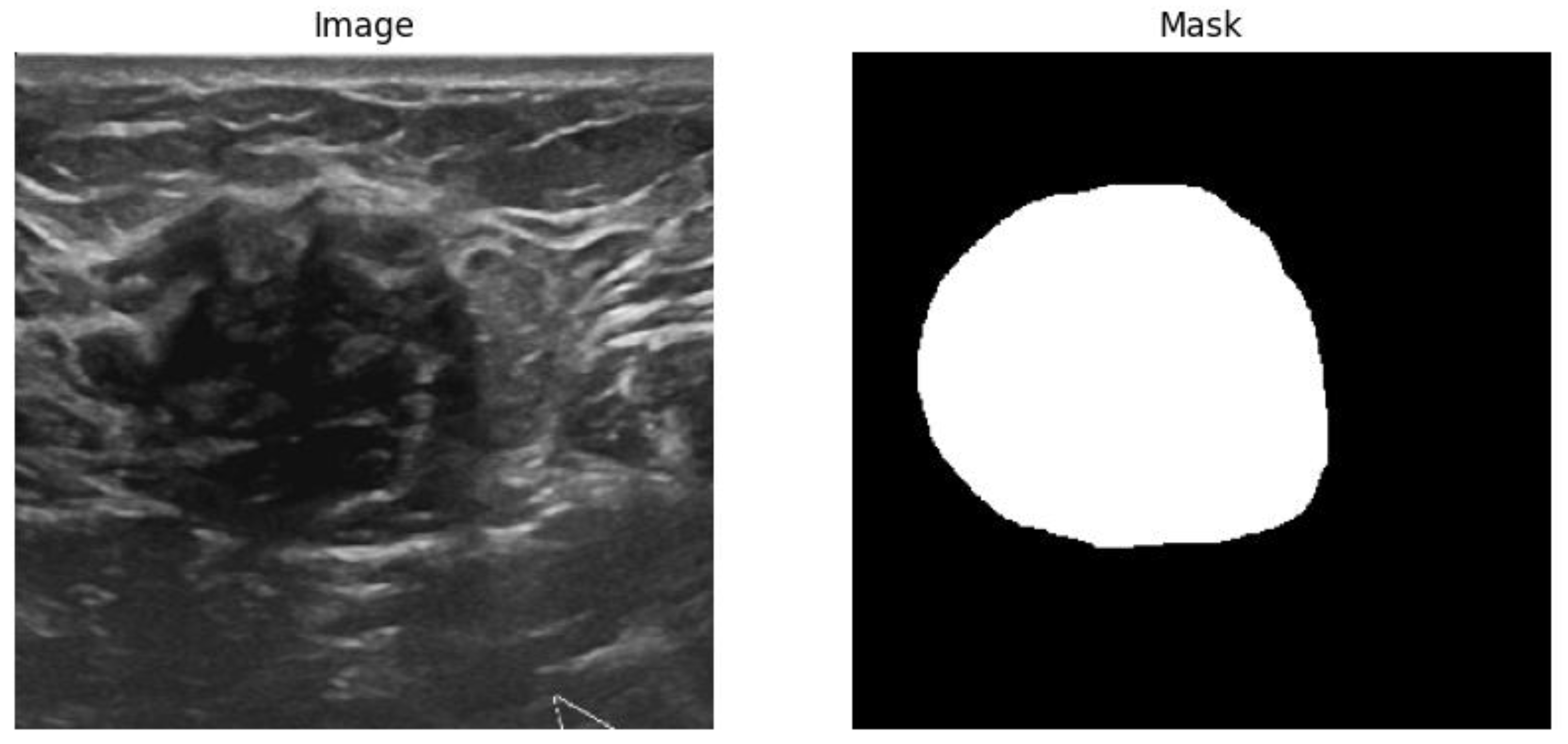
Figure 1.
Sample image and mask pair data for image segmentation task.
Figure 1.
Sample image and mask pair data for image segmentation task.
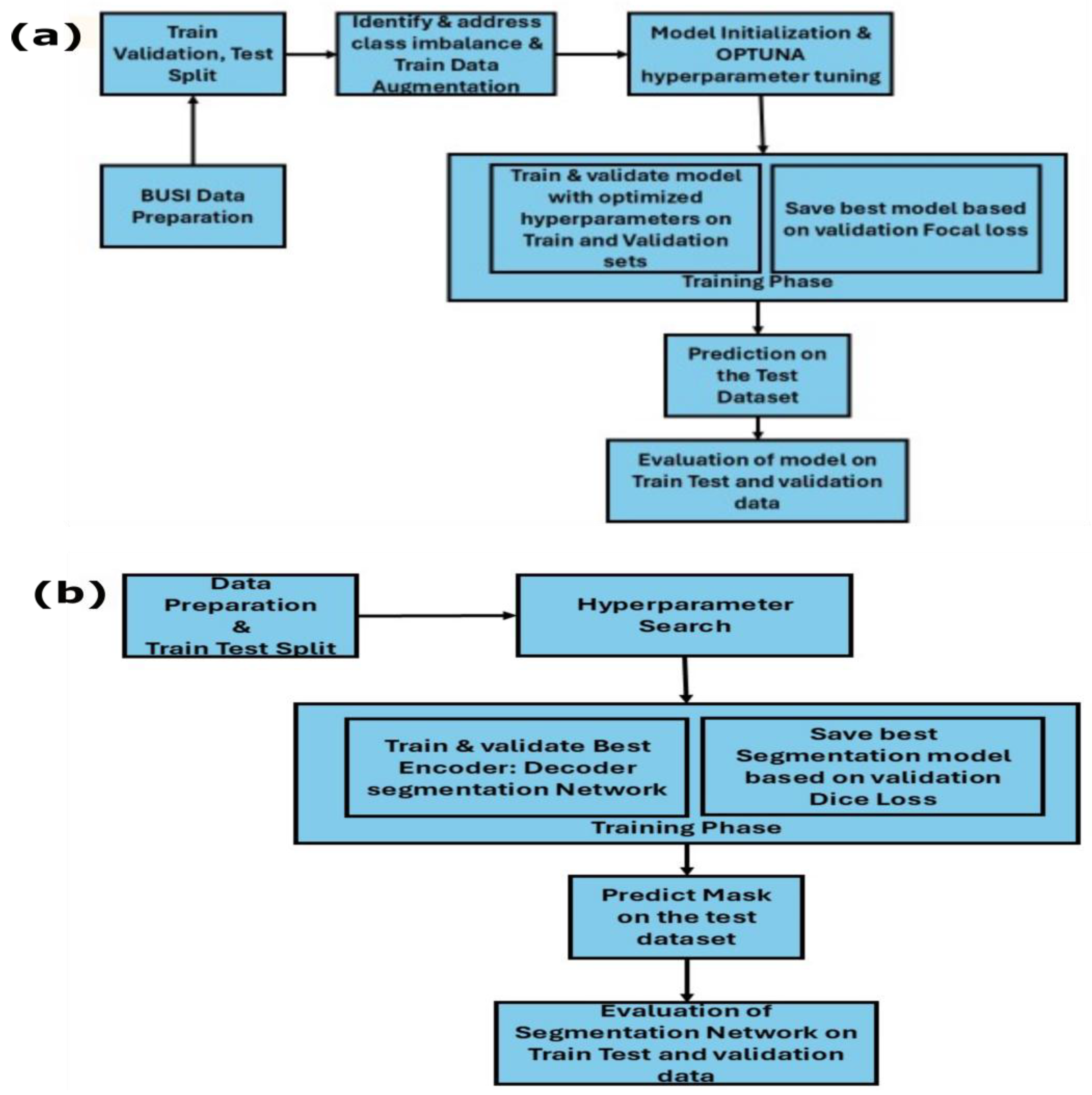
Figure 2.
(a) Breast cancer segmentation using encoder–decoder architecture. (b) Multiclass classification of breast cancer images.
Figure 2.
(a) Breast cancer segmentation using encoder–decoder architecture. (b) Multiclass classification of breast cancer images.
Figure 3.
U-Net architecture for medical image segmentation. The encoder progressively downsamples the input image through convolutional and max pooling layers, while the decoder upsamples feature maps through transposed convolutions and skip connections, producing a pixel-wise segmentation map [
30].
Figure 4.
U-Net++ architecture, demonstrating dense skip connections across multiple scales. The network features a nested encoder–decoder structure with sequential convolutional layers (
) connected through downsampling, upsampling and skip-connection pathways, enabling multi-scale feature extraction and fusion for improved segmentation [
33].
Figure 5.
DeepLabV3 architecture. The core ASPP module captures multi-scale context via parallel branches: (1) convolution, (2) three atrous convolutions with increasing dilation rates and (3) a global average pooling branch.
Figure 5.
DeepLabV3 architecture. The core ASPP module captures multi-scale context via parallel branches: (1) convolution, (2) three atrous convolutions with increasing dilation rates and (3) a global average pooling branch.
Figure 6.
Architecture of Frequency-Aware DeepLabV3 for semantic segmentation. The network consists of a Resnet encoder (blue), frequency enhancement module (yellow), feature fusion module with residual connection (pink), DeepLabV3 decoder with ASPP (green) and predicted mask (purple). The deepest encoder features undergo FFT-based decomposition into low-, mid- and high-frequency components, which are processed independently through convolutional layers with group normalization and dropout before fusion. A residual connection preserves spatial information while incorporating frequency-domain enhancements.
Figure 7.
Examples of data augmentation techniques, illustrating common geometric and photometric transformations applied to ultrasound images of the training set and its corresponding segmentation mask (green) for increasing dataset robustness. The displayed techniques are (a) horizontal flip, (b) vertical flip, (c) color jitter (a photometric alteration) and (d) rotation augmentation (geometric), all of which help deep learning models generalize better across variations in real-world data capture.
Figure 8.
Example predictions of the ground-truth mask by the Resent 18:U-Net model on the (a) train dataset, (b) validation dataset and (c) test dataset.
Figure 8.
Example predictions of the ground-truth mask by the Resent 18:U-Net model on the (a) train dataset, (b) validation dataset and (c) test dataset.
Figure 9.
Example predictions of the ground-truth mask by the Resent 18: U-Net++ model on the (a) training dataset, (b) validation dataset and (c) test dataset.
Figure 9.
Example predictions of the ground-truth mask by the Resent 18: U-Net++ model on the (a) training dataset, (b) validation dataset and (c) test dataset.
Figure 10.
Example predictions of the ground-truth mask by the Resent 18:DeepLabV3 model on the (a) training dataset, (b) validation dataset and (c) test dataset.
Figure 10.
Example predictions of the ground-truth mask by the Resent 18:DeepLabV3 model on the (a) training dataset, (b) validation dataset and (c) test dataset.
Figure 11.
Example predictions of the ground-truth mask by the Resent 18: FADeepLabV3 model on the (a) training dataset, (b) validation dataset and (c) test dataset.
Figure 11.
Example predictions of the ground-truth mask by the Resent 18: FADeepLabV3 model on the (a) training dataset, (b) validation dataset and (c) test dataset.
Figure 12.
Confusion matrix with proportions for the ResNet18 model on (a) training data, (b) validation data and (c) test data. Each matrix compares the true label (actual class) against the predicted label (model output) for the three classes: benign, normal and malignant. Overall accuracy of 96% on the training set, which dropped to 88.9% on the validation set and 86.4% on the test set. Specifically for the malignant class, the model demonstrated high recall across all subsets, maintaining 93.8% on training data, 93.5% on the validation set and 96.9% on the critical test set.
Figure 13.
Confusion matrix with proportions for the InceptionV3 model on (a) training data, (b) validation data and (c) test data. Each matrix compares the true label (actual class) against the predicted label (model output) for the three classes: benign, normal and malignant. Overall accuracy reached 92.08% on the training set, decreased to 87.80% on the validation set and further declined to 74.00% on the test set. The malignant class demonstrated strong recall of 93.5% on training data but degraded to 94.7% on validation data and 76.3% on the test set, indicating overfitting tendencies.
Figure 14.
Confusion matrix with proportions for the DenseNet121 model on (a) training data, (b) validation data and (c) test data. The model achieved 86.80% overall accuracy on the training set, declining to 70.00% on validation data and improving to 90.00% on the test set. The malignant class showed 91.1% recall on training data, declining to 59.3% on validation data but recovering to 89.2% on the test set, demonstrating variable performance across datasets.
Figure 15.
Confusion matrix with proportions for the MobileNet model on (a) training data, (b) validation data and (c) test data. Overall accuracy reached 94.08% on training data, dropped significantly to 81.00% on validation data and further declined to 71.00% on the test set. The malignant class achieved an exceptional 97.0% recall on training data but degraded to 75.0% on validation data and 71.1% on the test set, indicating substantial performance degradation on unseen data.
Figure 16.
Confusion matrix with proportions for GoogleNet model on (a) training data, (b) validation data and (c) test data. Overall accuracy was 91.00% on training data, decreased to 73.00% on validation data and reached 78.00% on the test set. The malignant class maintained a strong 97.1% recall on training data but dropped to 65.6% on validation data and improved to 85.7% on the test set, showing inconsistent generalization performance across datasets.
Figure 17.
Comparison of models’ performance on training, validation and test datasets based on F1 score and accuracy.
Figure 17.
Comparison of models’ performance on training, validation and test datasets based on F1 score and accuracy.
Figure 18.
Samples of classification performance of five encoder architectures (ResNet18, InceptionV3, DenseNet121, MobileNetV3 and GoogleNet) across training, validation and test datasets. Green labels indicate correct predictions, while red labels denote misclassifications. The figure demonstrates each model’s ability to discriminate between normal, benign and malignant breast lesions in ultrasound images.
Figure 19.
Grad-CAM visualizations of model misclassifications. (a) Benign-to-normal: localized focal attention (yellow–orange hot spot) indicates underestimation of pathological significance. (b) Benign-to-malignant: diffuse dual hot spots reflect overinterpretation of lesion boundary features as malignancy indicators.
Table 1.
Data distribution of image-mask pairs for binary segmentation task.
Table 1.
Data distribution of image-mask pairs for binary segmentation task.
| Training Dataset | Validation Dataset | Test Dataset |
|---|
| Images | Masks | Images | Masks | Images | Masks |
| 624 | 624 | 77 | 77 | 77 | 77 |
Table 2.
Dataset distribution of the images for multiclass classification task.
Table 2.
Dataset distribution of the images for multiclass classification task.
| Ultrasound Breast Images | Training Dataset | Validation Dataset | Test Dataset |
|---|
| Benign | 350 | 43 | 43 |
| Malignant | 168 | 21 | 21 |
| Normal | 106 | 13 | 13 |
| Total | 624 | 77 | 77 |
Table 3.
Optuna hyperparameter optimization of segmentation models.
Table 3.
Optuna hyperparameter optimization of segmentation models.
| Encoder | Decoder | Learning Rate | Weight Decay | Batch Size | Optimizer | Image Size |
|---|
| Resnet18 | U-Net | 0.000081 | 0.000079 | 8 | Adam | 288 |
| Resnet18 | U-Net++ | 0.000155 | 1.09011 | 8 | RMSprop | 288 |
| Resnet18 | DeepLabV3 | 0.00019 | 0.00019 | 8 | AdamW | 256 |
Table 4.
Performance of segmentation models on training, validation and test datasets.
Table 4.
Performance of segmentation models on training, validation and test datasets.
| Encoder–Decoder | Dataset | Pixel Accuracy | Dice Coefficient | IoU | AUC Score |
|---|
| Resnet18:U-Net | Train | 0.97 | 0.86 | 0.76 | 0.91 |
| Validation | 0.96 | 0.76 | 0.62 | 0.85 |
| Test | 0.96 | 0.74 | 0.59 | 0.82 |
| Resnet18:U-Net++ | Train | 0.98 | 0.87 | 0.77 | 0.92 |
| Validation | 0.96 | 0.76 | 0.60 | 0.84 |
| Test | 0.97 | 0.83 | 0.71 | 0.91 |
| Resnet18:DeepLabV3 | Train | 0.98 | 0.87 | 0.78 | 0.93 |
| Validation | 0.97 | 0.80 | 0.67 | 0.87 |
| Test | 0.98 | 0.83 | 0.70 | 0.90 |
| Resnet18:FADeepLabv3 | Train | 0.97 | 0.84 | 0.71 | 0.98 |
| Validation | 0.96 | 0.75 | 0.65 | 0.97 |
| Test | 0.97 | 0.85 | 0.72 | 0.98 |
Table 5.
Optuna hyperparameter optimization of multiclass breast cancer classification models.
Table 5.
Optuna hyperparameter optimization of multiclass breast cancer classification models.
| Model | Optimizer | Learning Rate | Weight Decay | FL (α) * | FL (γ) * | Batch Size | | | F1 Score |
|---|
| Resnet18 | RMSprop | 0.0000491 | 0.00027 | 0.57 | 4.03 | 32 | N/A | N/A | 0.77 |
| InceptionV3 | Adam | 0.0000163 | 0.00009 | 0.33 | 4.41 | 16 | 0.84 | 0.98 | 0.83 |
| Densenet121 | RMSprop | 0.0000246 | 0.00060 | 0.65 | 3.55 | 32 | N/A | N/A | 0.87 |
| MobilenetV3 | AdamW | 0.0001120 | 0.00626 | 0.44 | 4.86 | 8 | 0.81 | 0.96 | 0.88 |
| GoogleNet | Adam | 0.0008705 | 0.00015 | 0.73 | 4.24 | 32 | 0.91 | 0.93 | 0.82 |
Table 6.
Performance of the breast cancer classifiers on the training, validation and test datasets.
Table 6.
Performance of the breast cancer classifiers on the training, validation and test datasets.
| Model | Dataset | F1 Score | Accuracy | Metric | Benign | Normal | Malignant | Macro AVG |
|---|
| Resnet18 | Train | 0.90 | 0.90 | Precision | 0.98 | 0.96 | 0.94 | 0.96 |
| Recall | 0.92 | 0.94 | 0.99 | 0.95 |
| F1 score | 0.95 | 0.95 | 0.95 | 0.95 |
| Test | 0.77 | 0.81 | Precision | 0.86 | 0.92 | 0.74 | 0.84 |
| Recall | 0.63 | 0.80 | 0.97 | 0.80 |
| F1 score | 0.73 | 0.86 | 0.84 | 0.81 |
| Validation | 0.81 | 0.82 | Precision | 0.89 | 0.89 | 0.91 | 0.89 |
| Recall | 0.89 | 0.84 | 0.94 | 0.89 |
| F1 score | 0.89 | 0.86 | 0.92 | 0.89 |
| InceptionV3 | Train | 0.91 | 0.91 | Precision | 0.92 | 0.85 | 0.94 | 0.90 |
| Recall | 0.85 | 0.99 | 0.93 | 0.92 |
| F1 score | 0.88 | 0.91 | 0.94 | 0.91 |
| Test | 0.86 | 0.83 | Precision | 0.61 | 1.0 | 0.72 | 0.78 |
| Recall | 0.67 | 0.78 | 0.76 | 0.74 |
| F1 score | 0.64 | 0.88 | 0.74 | 0.75 |
| Validation | 0.77 | 0.74 | Precision | 0.83 | 0.94 | 0.86 | 0.88 |
| Recall | 0.83 | 0.76 | 0.95 | 0.85 |
| F1 score | 0.83 | 0.84 | 0.90 | 0.86 |
| Densenet121 | Train | 0.86 | 0.85 | Precision | 0.96 | 0.76 | 0.78 | 0.83 |
| Recall | 0.81 | 0.94 | 0.91 | 0.89 |
| F1 score | 0.88 | 0.84 | 0.84 | 0.85 |
| Test | 0.82 | 0.82 | Precision | 0.79 | 0.94 | 0.94 | 0.89 |
| Recall | 0.86 | 0.94 | 0.89 | 0.90 |
| F1 score | 0.83 | 0.94 | 0.92 | 0.90 |
| Validation | 0.73 | 0.71 | Precision | 0.71 | 0.57 | 0.84 | 0.71 |
| Recall | 0.78 | 0.72 | 0.59 | 0.70 |
| F1 score | 0.75 | 0.63 | 0.70 | 0.69 |
| MobileNetV3 | Train | 0.93 | 0.94 | Precision | 0.94 | 0.93 | 0.94 | 0.94 |
| Recall | 0.89 | 0.93 | 0.97 | 0.93 |
| F1 score | 0.92 | 0.93 | 0.95 | 0.93 |
| Test | 0.71 | 0.71 | Precision | 0.45 | 0.93 | 0.90 | 0.76 |
| Recall | 0.79 | 0.65 | 0.71 | 0.72 |
| F1 score | 0.58 | 0.76 | 0.79 | 0.71 |
| Validation | 0.81 | 0.80 | Precision | 0.66 | 1.00 | 0.90 | 0.85 |
| Recall | 1.00 | 0.67 | 0.75 | 0.81 |
| F1 score | 0.79 | 0.80 | 0.82 | 0.80 |
| GoogleNet | Train | 0.91 | 0.91 | Precision | 0.95 | 0.93 | 0.86 | 0.92 |
| Recall | 0.80 | 0.93 | 0.97 | 0.90 |
| F1 score | 0.87 | 0.93 | 0.91 | 0.91 |
| Test | 0.78 | 0.77 | Precision | 0.77 | 0.83 | 0.77 | 0.79 |
| Recall | 0.74 | 0.67 | 0.86 | 0.75 |
| F1 score | 0.75 | 0.74 | 0.81 | 0.77 |
| Validation | 0.73 | 0.73 | Precision | 0.64 | 0.81 | 0.75 | 0.73 |
| Recall | 0.86 | 0.71 | 0.66 | 0.74 |
| F1 score | 0.73 | 0.76 | 0.70 | 0.73 |
Table 7.
Misclassification analysis of Resent18 on validation dataset.
Table 7.
Misclassification analysis of Resent18 on validation dataset.
| S.No | True Label | Predicted Label | Normal Probability | Benign Probability | Malignant Probability |
|---|
| 1 | 0 | 1 | 0.38 | 0.42 | 0.20 |
| 2 | 0 | 1 | 0.32 | 0.44 | 0.24 |
| 3 | 0 | 1 | 0.35 | 0.38 | 0.27 |
| 4 | 1 | 2 | 0.10 | 0.39 | 0.51 |
| 5 | 2 | 0 | 0.81 | 0.02 | 0.17 |
| 6 | 1 | 2 | 0.10 | 0.39 | 0.51 |
| 7 | 2 | 0 | 0.81 | 0.02 | 0.17 |
| 8 | 1 | 2 | 0.10 | 0.39 | 0.51 |
| 9 | 2 | 0 | 0.81 | 0.02 | 0.17 |

 ,
, 


