
On Data Selection and Regularization for Underdetermined Vibro-Acoustic Source Identification

Abstract
1. Introduction
2. Brief Descriptions in the Theoretical Backgrounds
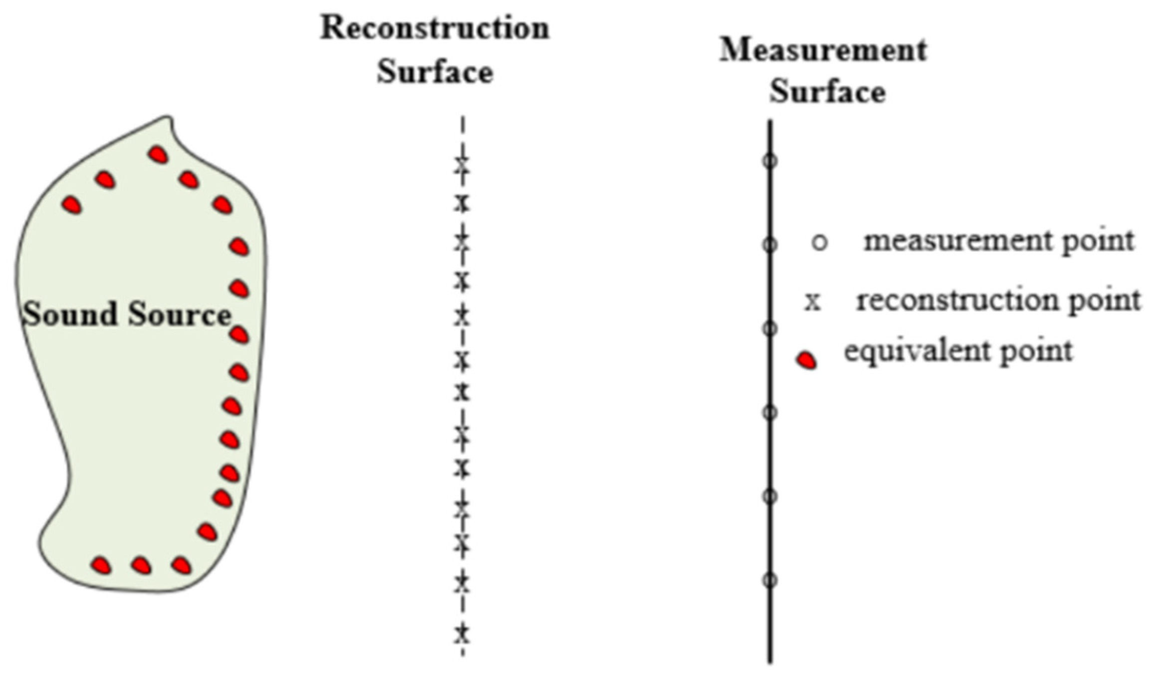
2.1. NAH Based on the ESM
2.2. Preparation of Meaningful Underdetermined Hologram Data
2.2.1. Sequential Elimination of the Most Dependent Positions
2.2.2. Sequential Elimination of Measuring Points Yielding the Smallest Singular Values
2.2.3. Expansion of the Patch Hologram Data with Zero Padding
2.3. Regularization of the Inverse Operation Using the Underdetermined Hologram Data
2.3.1. Tikhonov Regularization Adapting the GCV
2.3.2. Statistical Regularization Based on the Bayesian Technique
2.3.3. Regularization Using the Data Compression Technique
3. Numerical Test
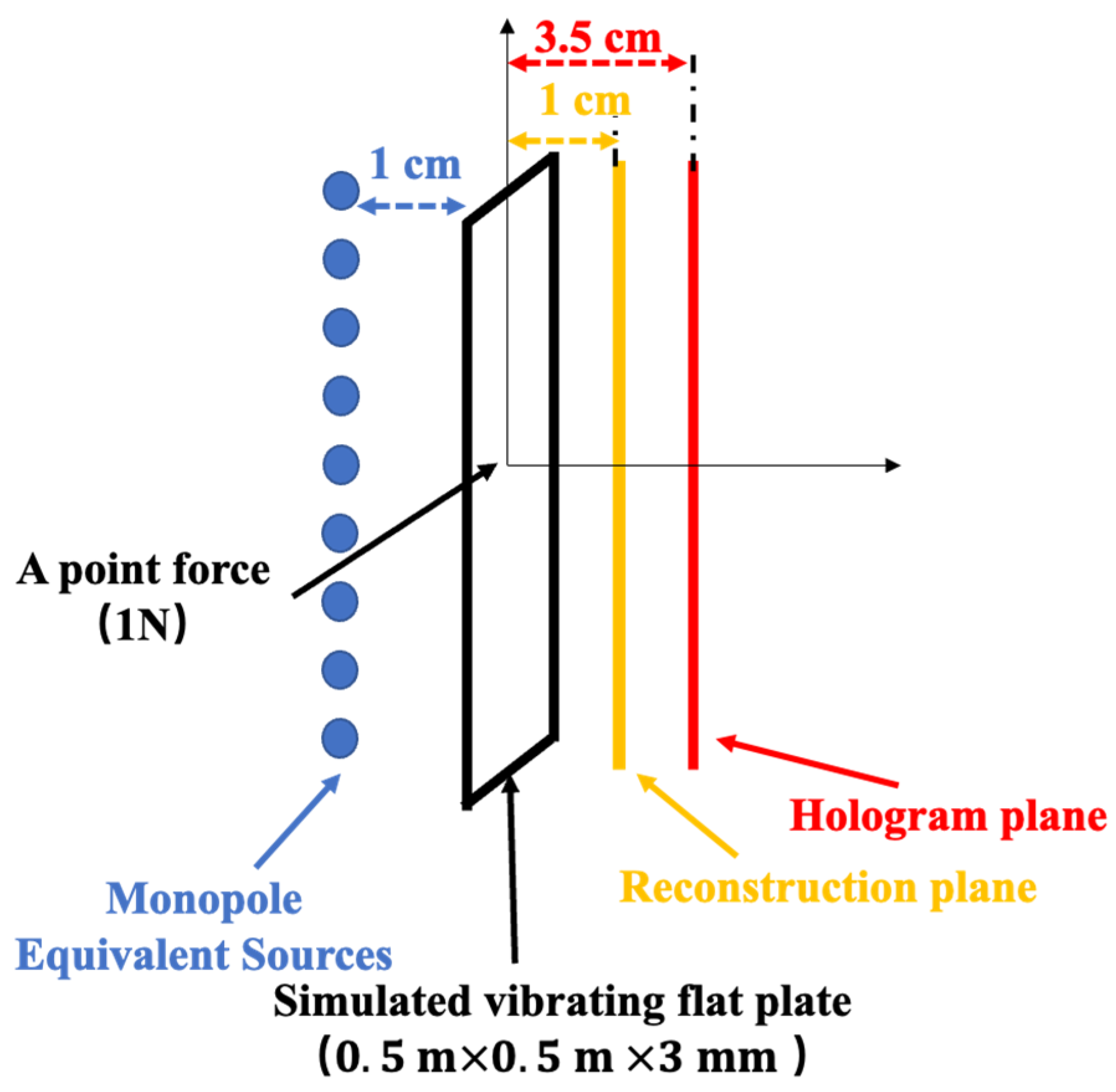
3.1. Test Model and Selection of Measurement Points
3.2. Comparison of the Layout of the Measurement Points
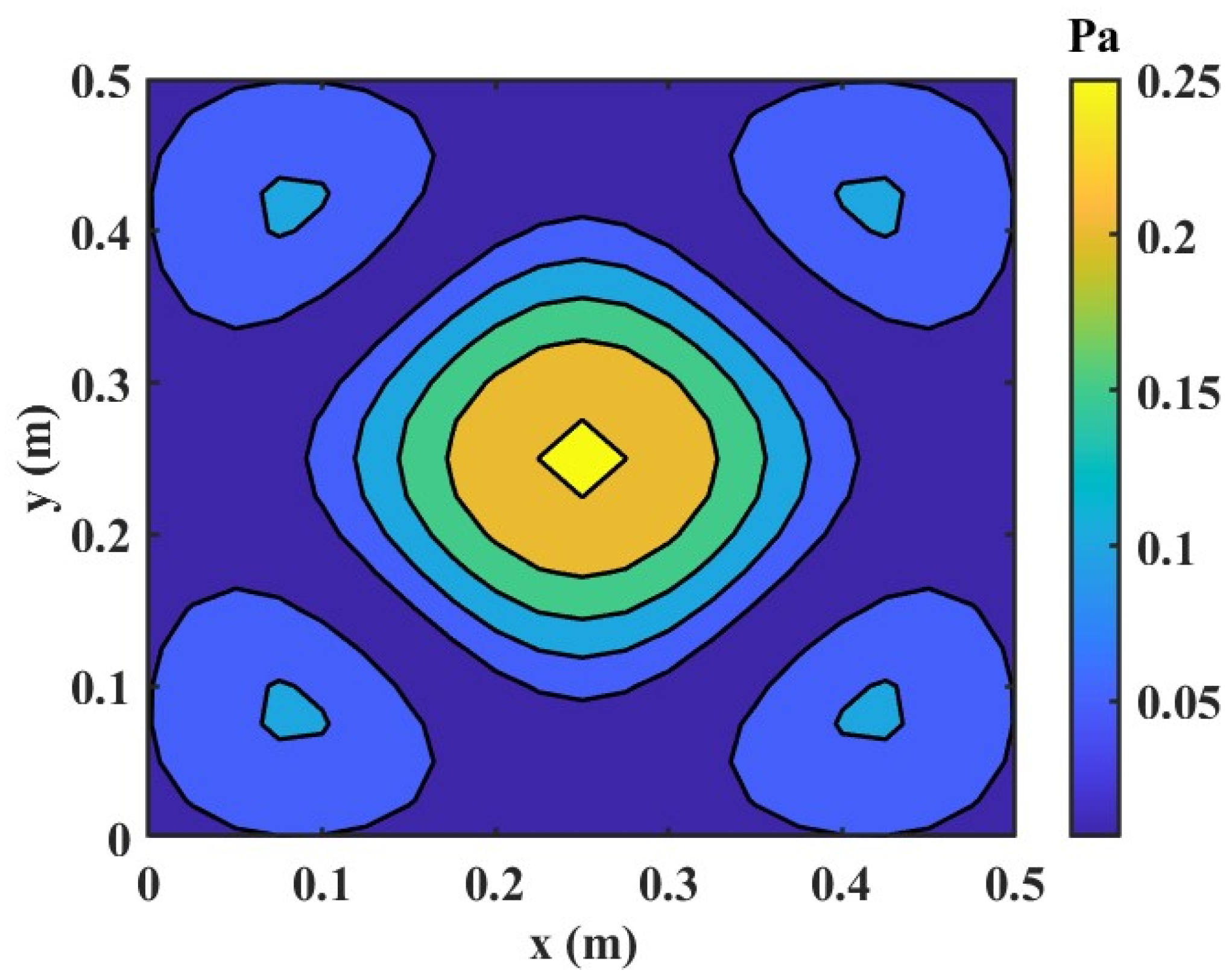
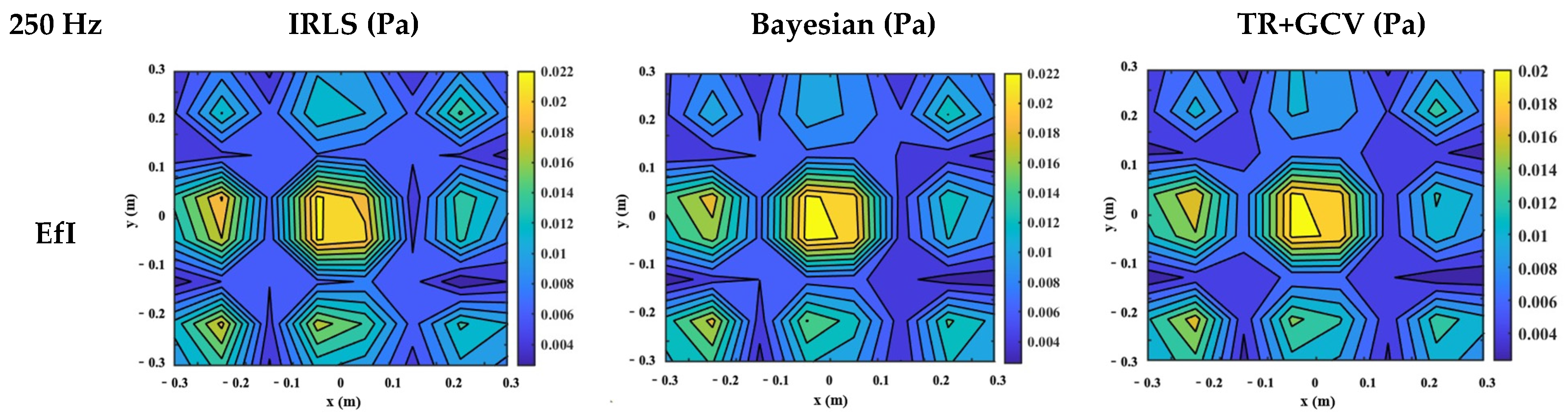
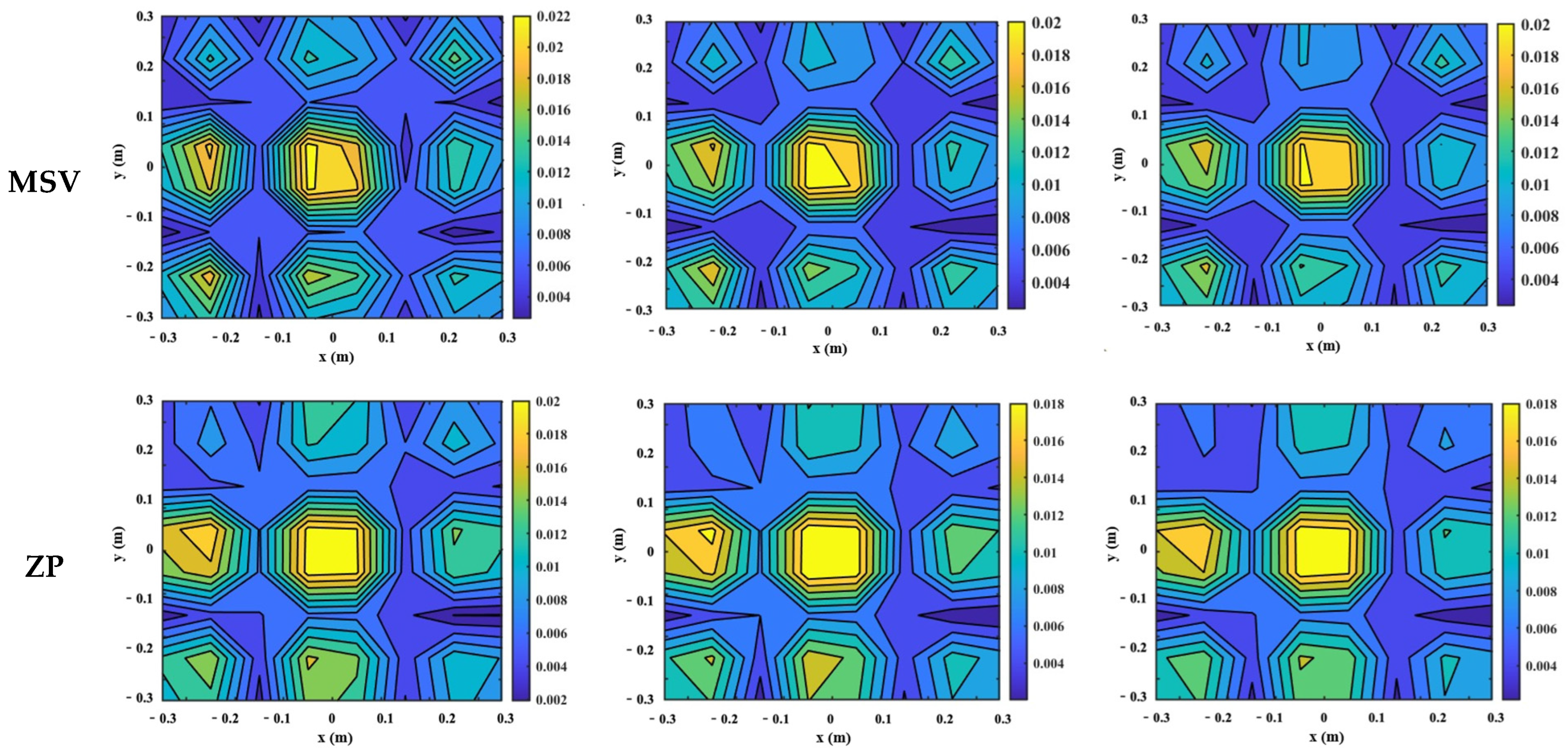
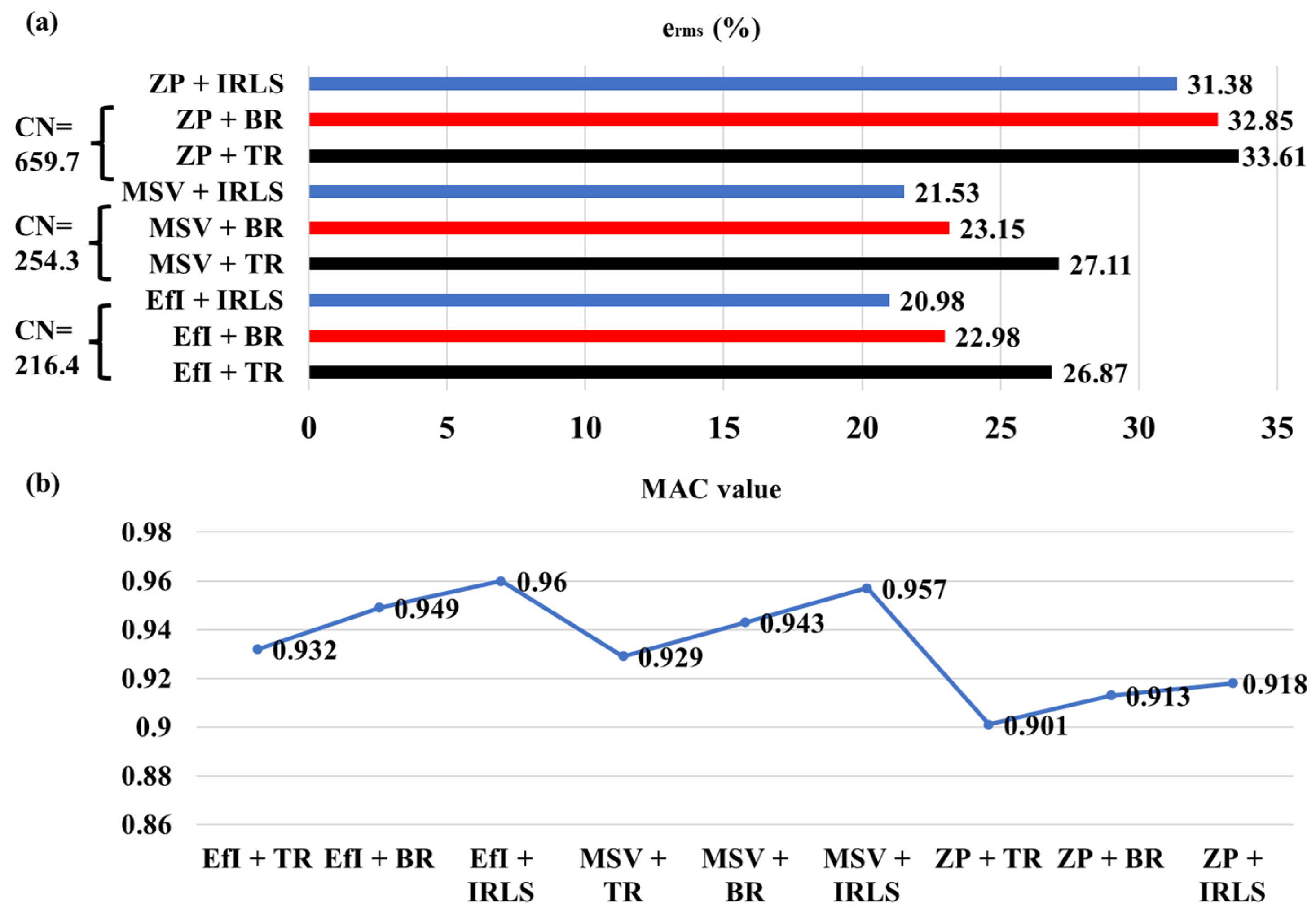
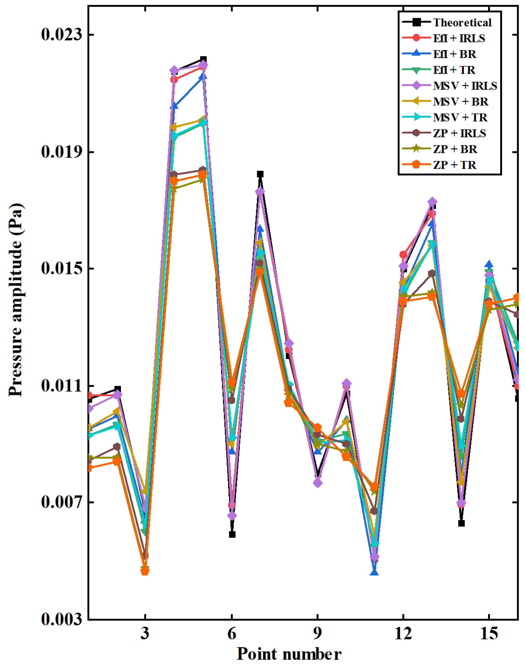
3.3. Reconstruction of Source Field Using the Regularization
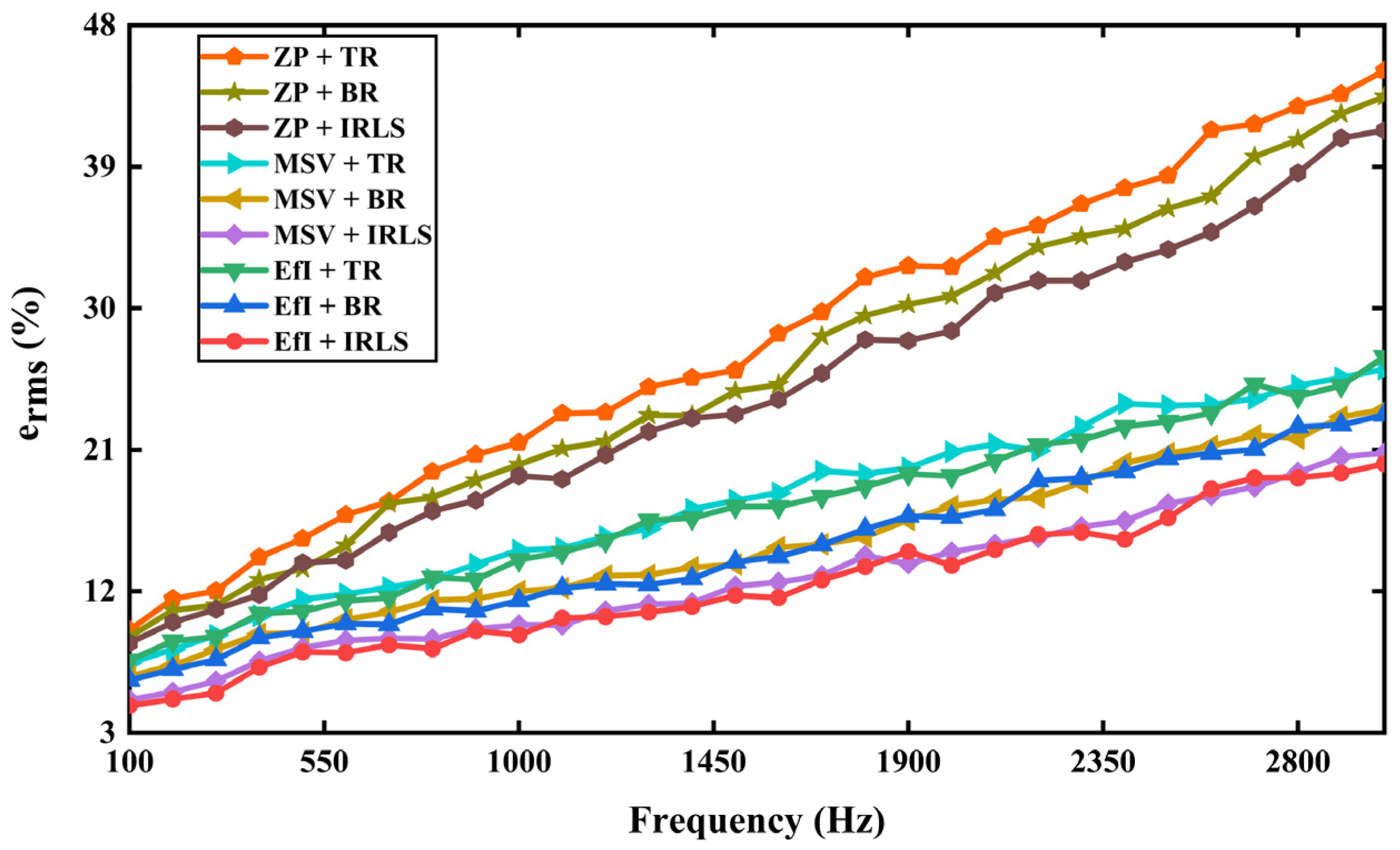
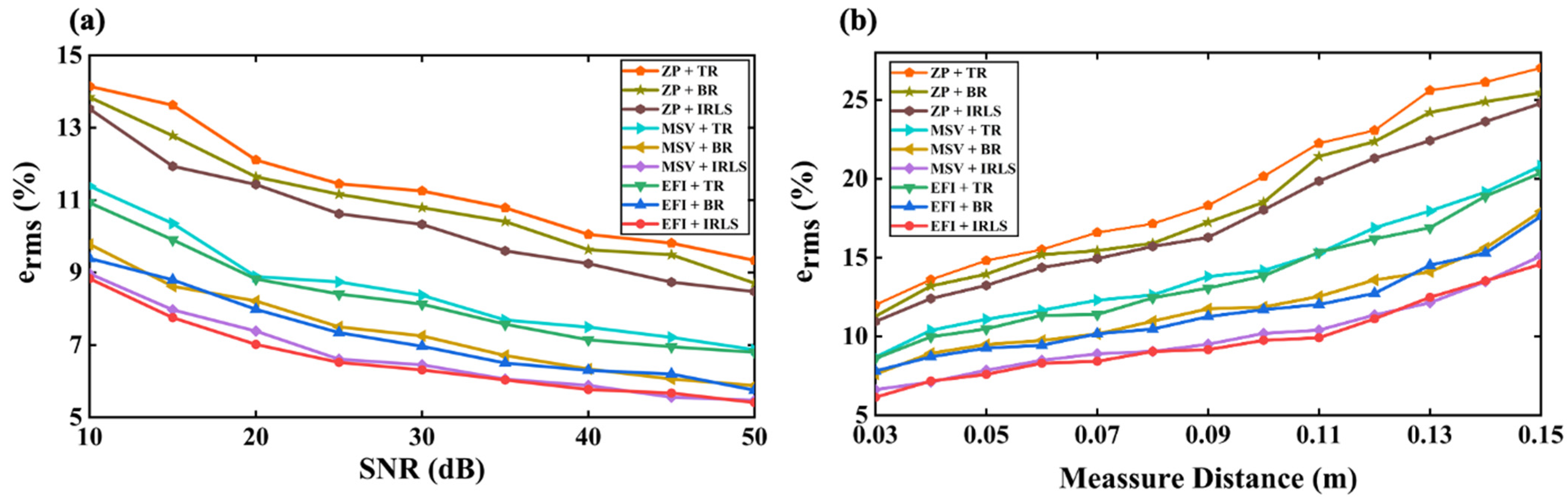
3.4. Effects of SNR and Measuring Distance
4. Experimental Test
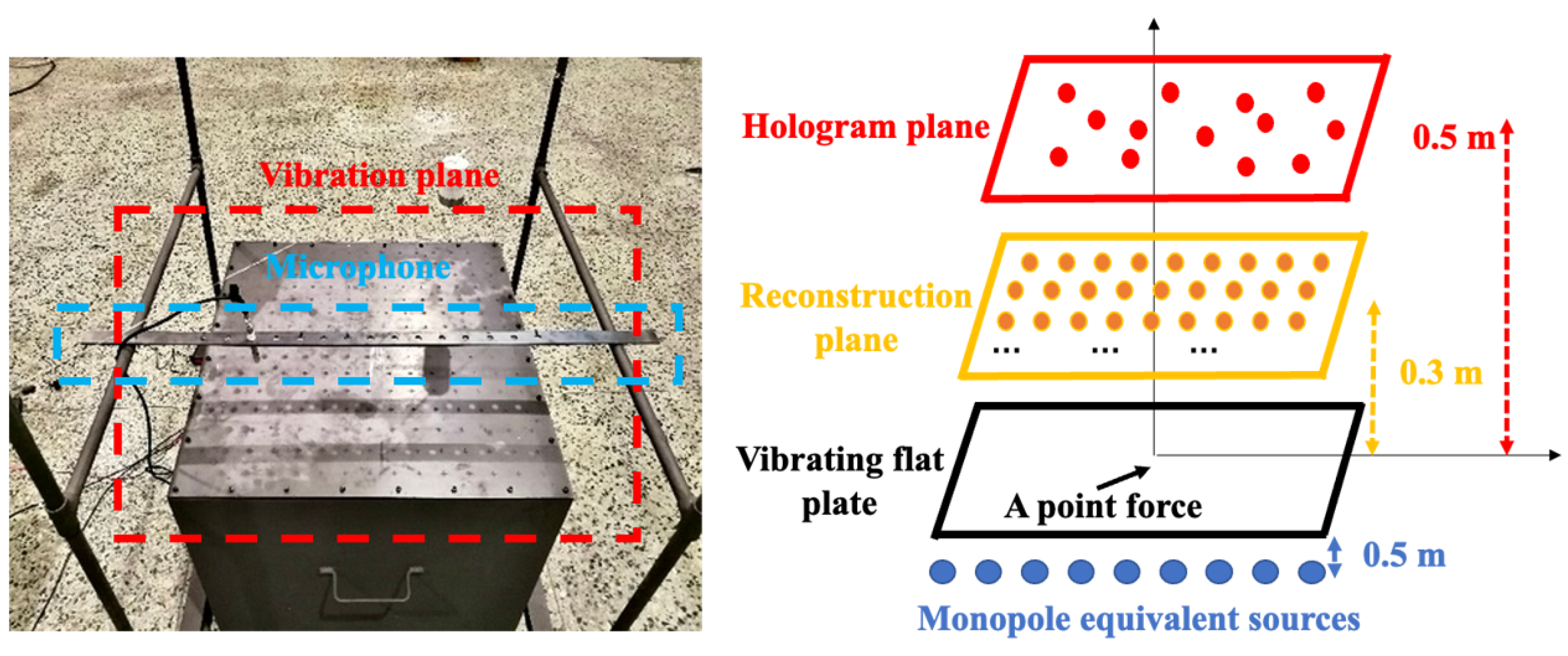
4.1. Test Setup and Method
- (1)
- The experimental bench and measuring device was installed.
- (2)
- A signal was given to the vibration exciter separately and the pressure was measured on the hologram surface.
- (3)
- The radiated pressure on the reconstruction plane was measured at 0.05 m above the steel plate as the actual value for comparison.
- (4)
- After processing the corresponding data, it was imported into the analyzer, where the computer processed the analyzed results.
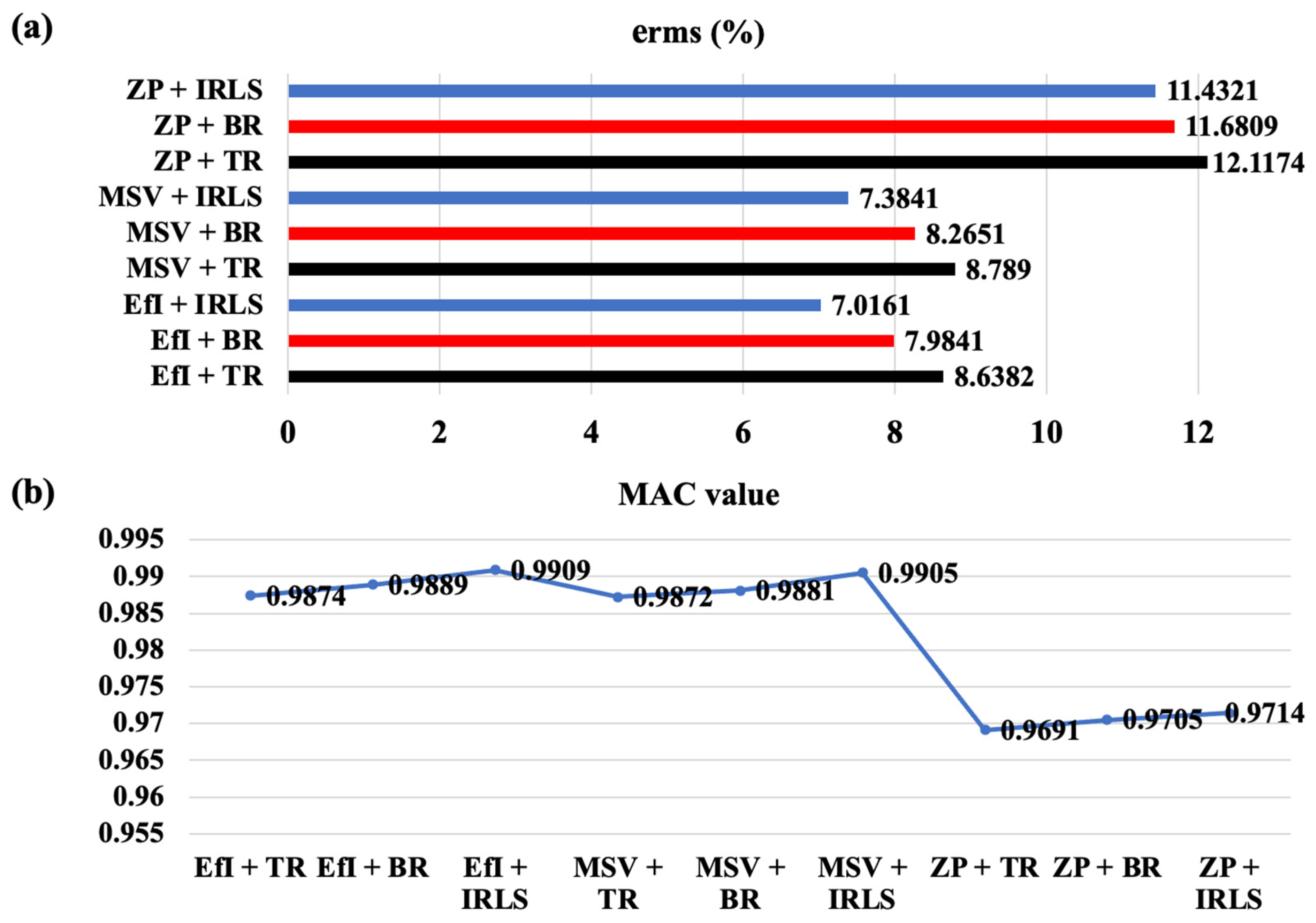
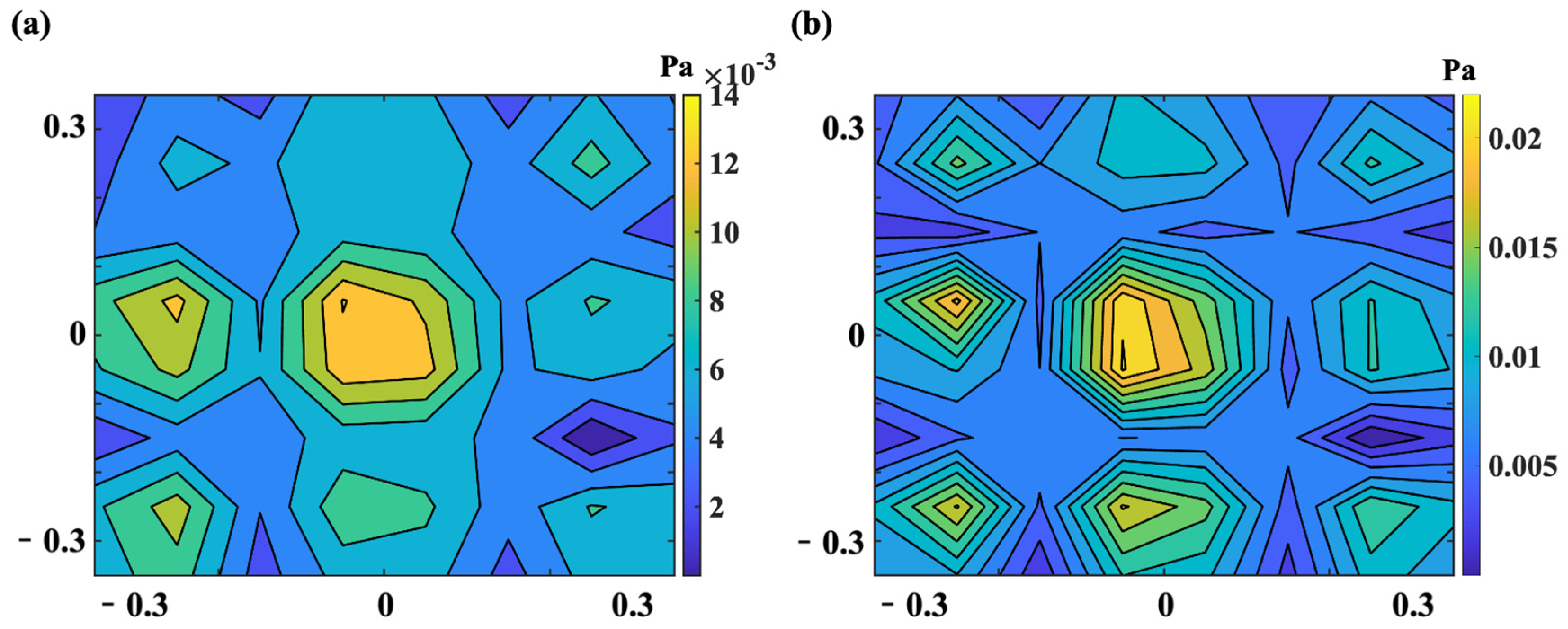
4.2. Test Result
5. Conclusions
Author Contributions
Funding
Institutional Review Board Statement
Informed Consent Statement
Data Availability Statement
Conflicts of Interest
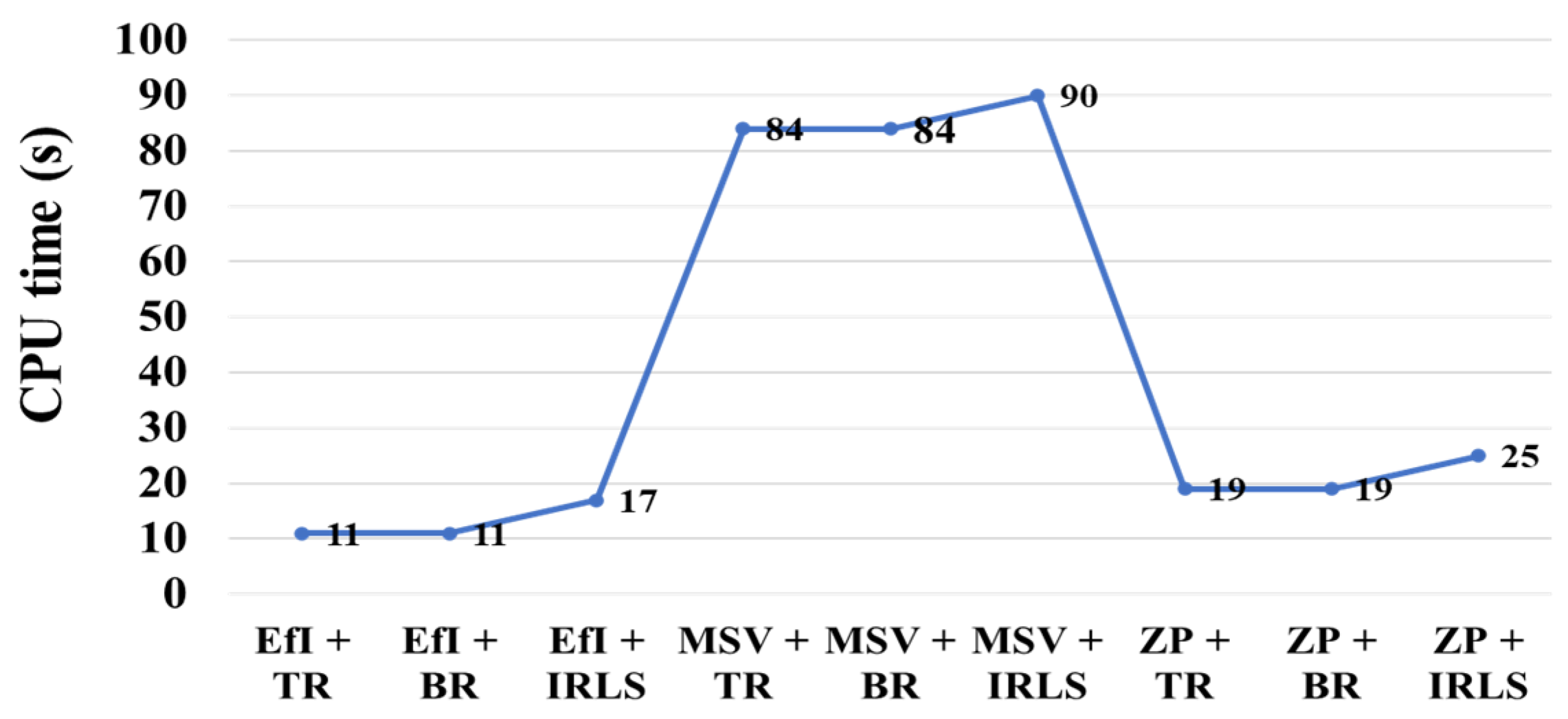
Appendix A. Comparison of CPU Time
References
- Williams, E.G.; Maynard, J.D. Holographic imaging without the wavelength resolution limit. Phys. Rev. Lett. 1980, 45, 554–557. [Google Scholar] [CrossRef]
- Gardner, B.K.; Bernhard, R.J. A noise source identification technique using an inverse Helmholtz integral equation method. J. Vib. Acoust. 1988, 110, 84–90. [Google Scholar] [CrossRef]
- Williams, E.G. Fourier Acoustics: Sound Radiation and Near-Field Acoustical Holography; Academic Press: Cambridge, MA, USA, 1999. [Google Scholar]
- Wang, Z.; Wu, S.F. Helmholtz equation-least-squares method for reconstructing the acoustic pressure field. J. Acoust. Soc. Am. 1997, 102, 2020–2032. [Google Scholar] [CrossRef]
- Bi, C.X.; Dong, B.C.; Zhang, X.Z.; Zhang, Y.B. Equivalent source method-based near-field acoustic holography in a moving medium. J. Vib. Acoust. 2017, 139, 051017. [Google Scholar] [CrossRef]
- Jiang, L.X.; Xiao, Y.H.; Zou, G.P.; Ih, J.G. Optimal sensor positioning for the sparse measurement in the acoustic reconstruction of a large source. IEEE Trans. Instrum. Meas. 2023, 72, 6502513. [Google Scholar] [CrossRef]
- Tikhonov, A.N. Solution of incorrectly formulated problems and the regularization method. Sov. Math. Dokl. 1963, 4, 1035–1038. [Google Scholar]
- Golub, G.H.; Heath, M.; Wahba, G. Generalized cross-validation as a method for choosing a good ridge parameter. Technometrics 1979, 21, 215–223. [Google Scholar] [CrossRef]
- Hansen, P.C.; O’Leary, D.P. The use of the L-curve in the regularisation of discrete ill-posed problems. SIAM J. Sci. Stat. Comput. 1993, 14, 1487–1503. [Google Scholar] [CrossRef]
- Kim, B.K.; Ih, J.G. Design of an optimal wave-vector filter for enhancing the resolution of reconstructed source field by near-field acoustical holography (NAH). J. Acoust. Soc. Am. 2000, 107, 3289–3297. [Google Scholar] [CrossRef]
- Chardon, G.; Daudet, L.; Peillot, A.; Ollivier, F.; Bertin, N.; Gribonval, R. Near-field acoustic holography using sparse regularization and compressive sampling principles. J. Acoust. Soc. Am. 2012, 132, 1521–1534. [Google Scholar] [CrossRef]
- Fernandez-Grande, E.; Xenaki, A. The equivalent source method as a sparse signal reconstruction. In Proceedings of the Inter-Noise, San Francisco, CA, USA, 9–12 August 2015. [Google Scholar]
- Fernandez-Grande, E.; Xenaki, A.; Gerstoft, P. A sparse equivalent source method for near-field acoustic holography. J. Acoust. Soc. Am. 2017, 141, 532–542. [Google Scholar] [CrossRef] [PubMed]
- Bi, C.X.; Liu, Y.; Xu, L.; Zhang, Y.B. Sound field reconstruction using compressed modal equivalent point source method. J. Acoust. Soc. Am. 2017, 141, 73–79. [Google Scholar] [CrossRef]
- Hald, J. Fast wideband acoustical holography. J. Acoust. Soc. Am. 2016, 139, 1508–1517. [Google Scholar] [CrossRef]
- Bai, M.R.; Chun, C.; Shih-Syuan, L. Iterative algorithm for solving acoustic source characterization problems under block sparsity constraints. J. Acoust. Soc. Am. 2018, 143, 3747–3757. [Google Scholar] [CrossRef]
- Grant, M.; Boyd, S. CVX: Matlab Software for Disciplined Convex Programming, Version 1.21; CVX Research: Austin, TX, USA, 2011. Available online: http://cvxr.com/cvx (accessed on 13 July 2021).
- Hald, J. A comparison of iterative sparse equivalent source methods for near-field acoustical holography. J. Acoust. Soc. Am. 2018, 143, 3758–3769. [Google Scholar] [CrossRef]
- Kim, B.K.; Ih, J.G. On the reconstruction of vibro-acoustic field over the surface enclosing an interior space using the boundary element method. J. Acoust. Soc. Am. 1996, 100, 3003–3016. [Google Scholar] [CrossRef]
- Kammer, D.C. Sensor placement for on-orbit modal identification and correlation of large space structures. J. Guid. Control Dyn. 1991, 14, 251–259. [Google Scholar] [CrossRef]
- Lee, M.Y.; Bolton, J.S. Patch near-field acoustical holography in cylindrical geometry. J. Acoust. Soc. Am. 2005, 118, 3721–3732. [Google Scholar] [CrossRef]
- Pascal, J.C.; Paillasseur, S.; Thomas, J.H.; Li, J.F. Patch near-field acoustic holography: Regularized extension and statistically optimized methods. J. Acoust. Soc. Am. 2009, 126, 1264–1268. [Google Scholar] [CrossRef]
- Hald, J. Planar near-field acoustical holography with arrays smaller than the sound source. In Proceedings of the 17th International Congress on Acoustics (ICA), Rome, Italy, 2–7 September 2001; Volume I. Pt. A. [Google Scholar]
- Sarkissian, A. Method of superposition applied to patch near-field acoustical holography. J. Acoust. Soc. Am. 2005, 118, 671–678. [Google Scholar] [CrossRef]
- Pereira, A.; Leclere, Q. Improving the equivalent source method for noise source identification in enclosed spaces. In Proceedings of the 18th International Congress on Sound and Vibration 2011 (ICSV 18), Rio de Janeiro, Brazil, 10–14 July 2011. [Google Scholar]
- Antoni, J. A Bayesian approach to sound source reconstruction: Optimal basis, regularization, and focusing. J. Acoust. Soc. Am. 2012, 131, 2873–2890. [Google Scholar] [CrossRef] [PubMed]
- Hu, D.Y.; Liu, X.Y.; Xiao, Y.; Fang, Y. Fast sparse reconstruction of sound field via Bayesian compressive sensing. J. Vib. Acoust. 2019, 141, 041017. [Google Scholar] [CrossRef]
- Koopmann, G.H.; Song, L.; Fahnline, J. A method for computing acoustic fields based on the principle of wave superposition. J. Acoust. Soc. Am. 1989, 86, 2433–2438. [Google Scholar] [CrossRef]
- Jiang, L.X.; Xiao, Y.H.; Zou, G.P. Data extension near-field acoustic holography based on improved regularization method for resolution enhancement. Appl. Acoust. 2019, 156, 128–141. [Google Scholar] [CrossRef]
- Williams, E.G. Regularization methods for near-field acoustical holography. J. Acoust. Soc. Am. 2001, 110, 1976–1988. [Google Scholar] [CrossRef]
- Yoon, S.H.; Nelson, P.A. Estimation of acoustic source strength by inverse methods: Part II, experimental investigation of methods for choosing regularization parameters. J. Sound Vib. 2000, 233, 665–701. [Google Scholar] [CrossRef]
- Bai, M.R.; Ih, J.G.; Benesty, J. Acoustic Array Systems: Theory, Implementation, and Application; John Wiley: Hoboken, NJ, USA, 2013. [Google Scholar]
- Gomes, J.; Hansen, P.C. A study on regularization parameter choice in near-field acoustical holography. J. Acoust. Soc. Am. 2008, 123, 3385. [Google Scholar] [CrossRef]
- Welch, P.D. The use of fast Fourier transform for the estimation of power spectra: A method based on time averaging over short, modified periodograms. IEEE Trans. Audio Electroacoust. 1967, 2, 70–73. [Google Scholar] [CrossRef]
 is the measurement points, and
  is the padding points.
is the measurement points, and is the padding points.
is the padding points.
is the measurement points, and is the padding points.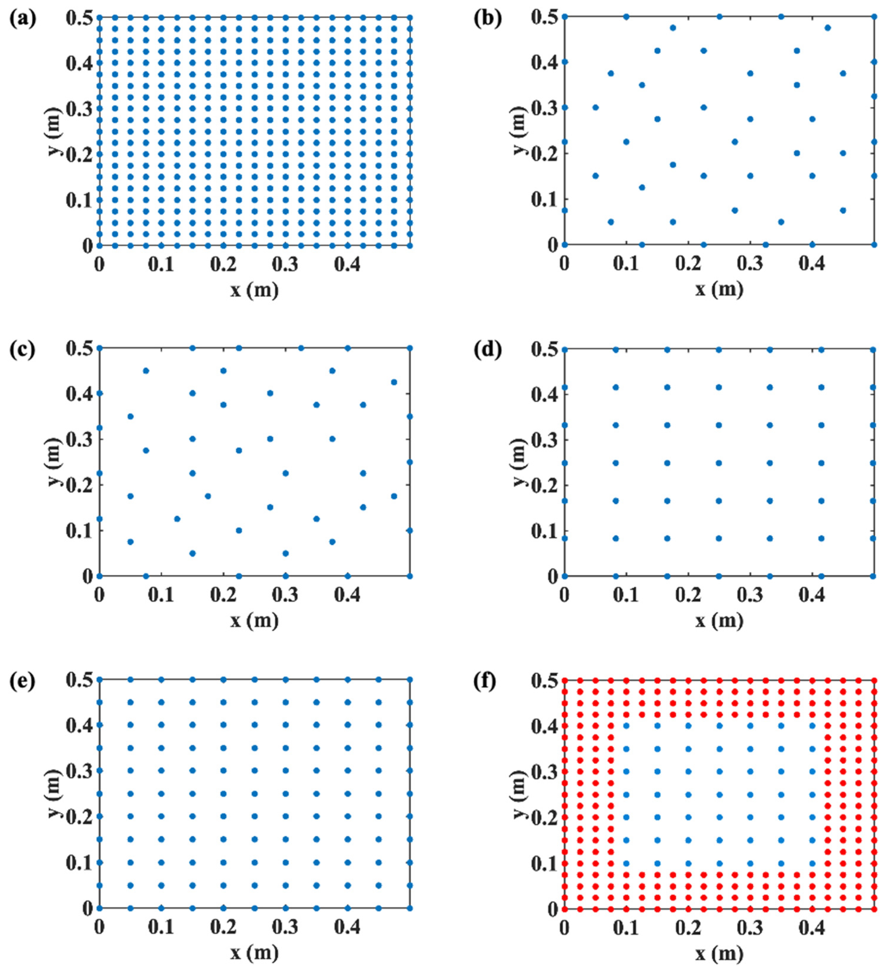
 , selected by the EfI method;
  , selected by the MSV method;
  , evenly spaced points;
  , evenly spaced 49 points with zero padding;
  , evenly spaced 121 points.
, selected by the EfI method; , selected by the MSV method; , evenly spaced points; , evenly spaced 49 points with zero padding; , evenly spaced 121 points.
, evenly spaced 121 points.
, selected by the EfI method; , selected by the MSV method; , evenly spaced points; , evenly spaced 49 points with zero padding; , evenly spaced 121 points.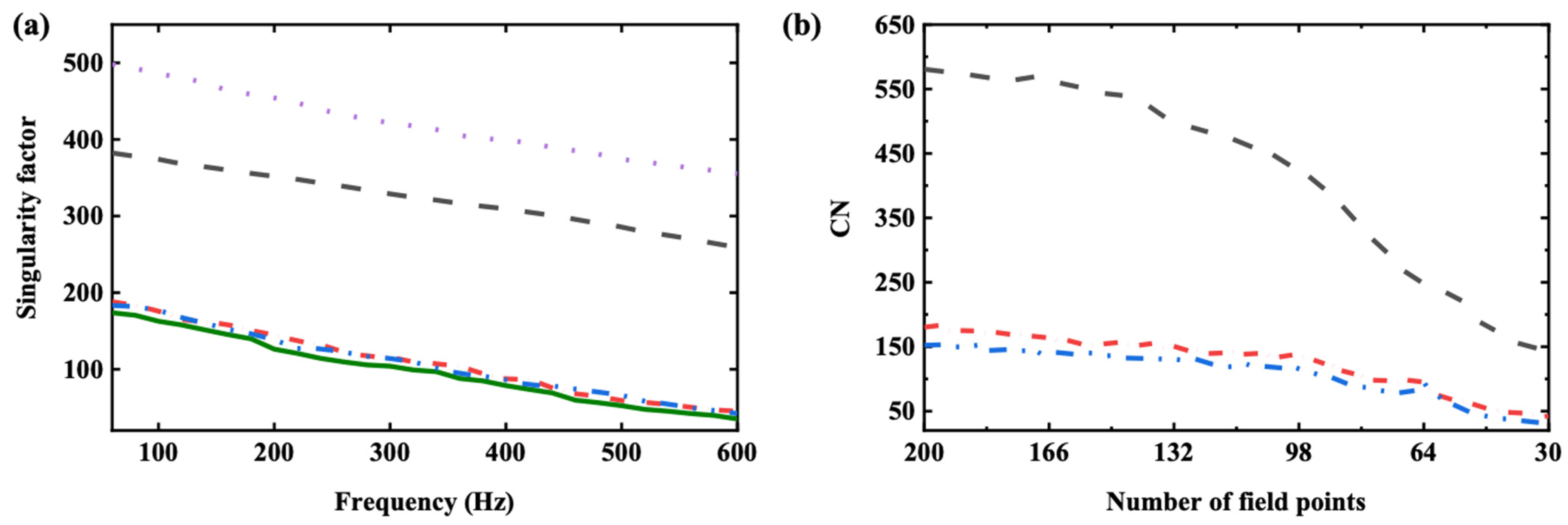
 , selected by the EfI method;
  , selected by the MSV method;
  , evenly spaced 49 points.
, selected by the EfI method; , selected by the MSV method; , evenly spaced 49 points.
, evenly spaced 49 points.
, selected by the EfI method; , selected by the MSV method; , evenly spaced 49 points.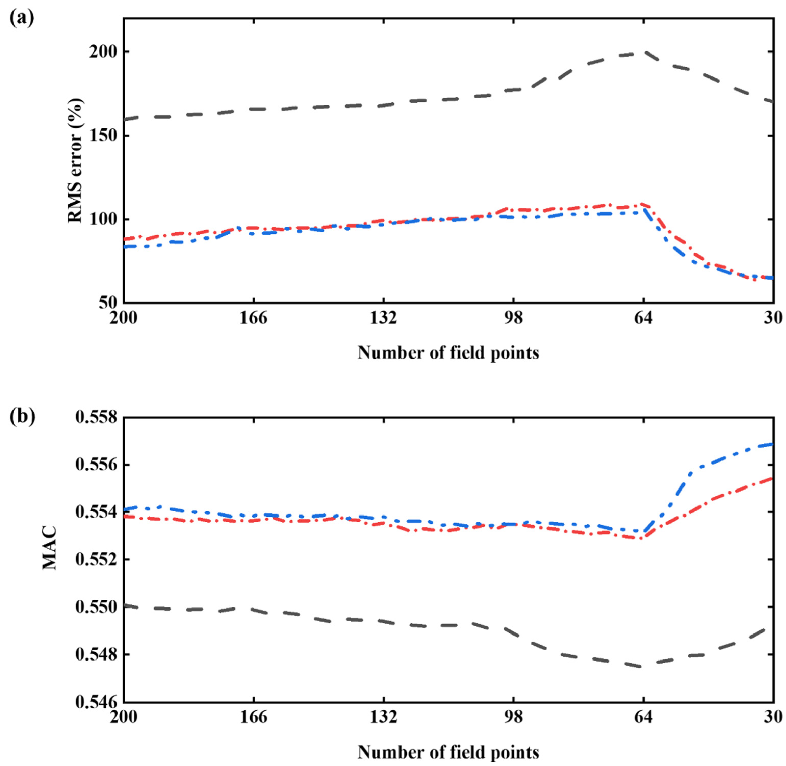
 is the measurement points, and is the padding points.
is the measurement points, and is the padding points.
is the measurement points, and is the padding points.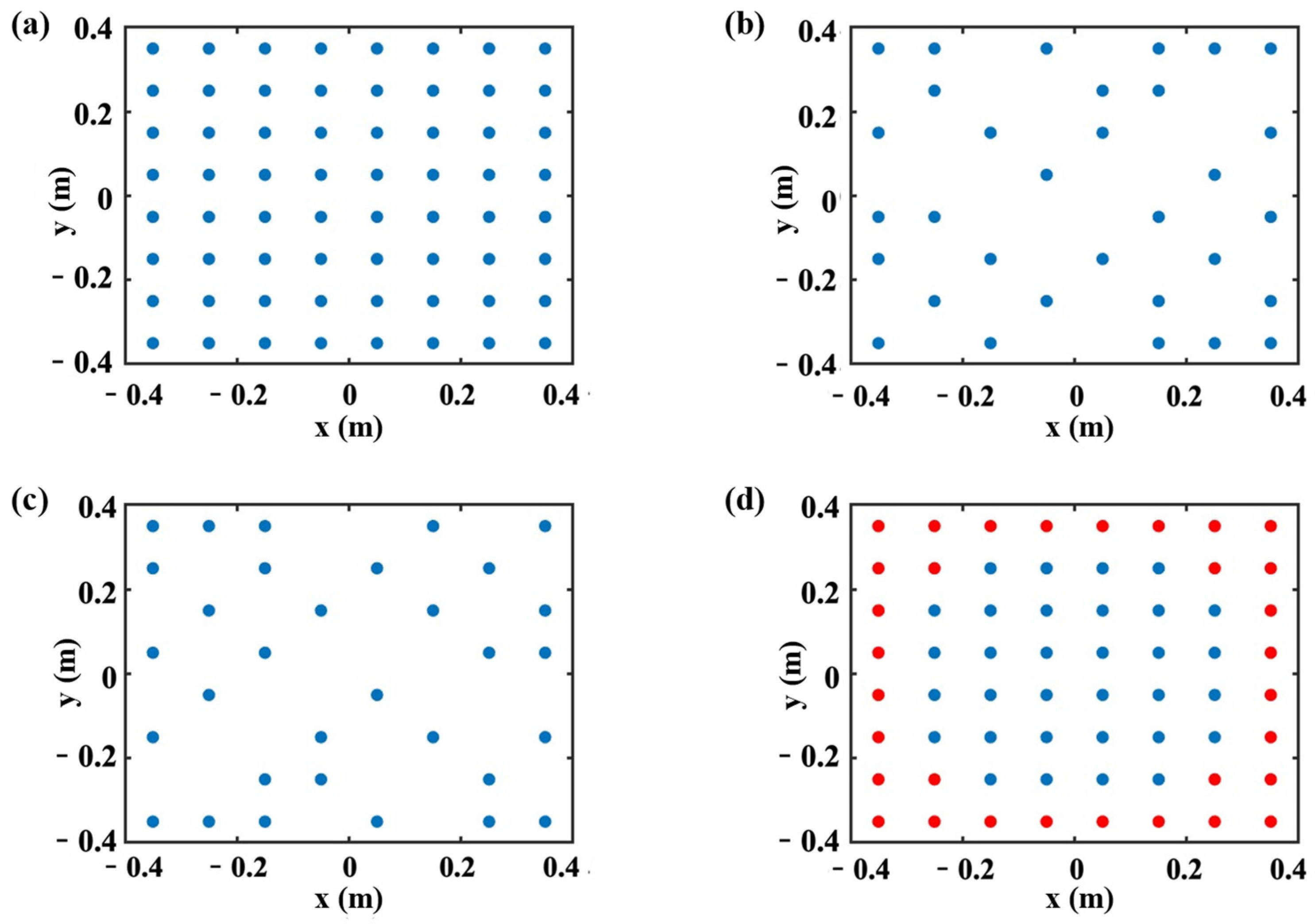

| Mode Index | 1 | 2 | 3 | 4 | 5 | 6 | 7 |
|---|---|---|---|---|---|---|---|
| (m, n) | (1, 1) | (1, 2) | (2, 1) | (2, 2) | (2, 3) | (3, 2) | (3, 3) |
| Frequency (Hz) | 59 Hz | 147 Hz | 147 Hz | 235 Hz | 385 Hz | 385 Hz | 528 Hz |
Disclaimer/Publisher’s Note: The statements, opinions and data contained in all publications are solely those of the individual author(s) and contributor(s) and not of MDPI and/or the editor(s). MDPI and/or the editor(s) disclaim responsibility for any injury to people or property resulting from any ideas, methods, instructions or products referred to in the content. |
© 2025 by the authors. Licensee MDPI, Basel, Switzerland. This article is an open access article distributed under the terms and conditions of the Creative Commons Attribution (CC BY) license (https://creativecommons.org/licenses/by/4.0/).
Share and Cite
Jiang, L.; Liu, J.; Jiang, X.; Pang, Y. On Data Selection and Regularization for Underdetermined Vibro-Acoustic Source Identification. Sensors 2025, 25, 3767. https://doi.org/10.3390/s25123767
Jiang L, Liu J, Jiang X, Pang Y. On Data Selection and Regularization for Underdetermined Vibro-Acoustic Source Identification. Sensors. 2025; 25(12):3767. https://doi.org/10.3390/s25123767
Chicago/Turabian StyleJiang, Laixu, Jingqiao Liu, Xin Jiang, and Yuezhao Pang. 2025. "On Data Selection and Regularization for Underdetermined Vibro-Acoustic Source Identification" Sensors 25, no. 12: 3767. https://doi.org/10.3390/s25123767
APA StyleJiang, L., Liu, J., Jiang, X., & Pang, Y. (2025). On Data Selection and Regularization for Underdetermined Vibro-Acoustic Source Identification. Sensors, 25(12), 3767. https://doi.org/10.3390/s25123767