
An Anti-Forensics Video Forgery Detection Method Based on Noise Transfer Matrix Analysis


Abstract
1. Introduction
- Multiple recoding traces are solid proof of a loss of originality. However, multiple recoding traces may not indicate that the video has necessarily been tampered with for reasonable transmission processes.
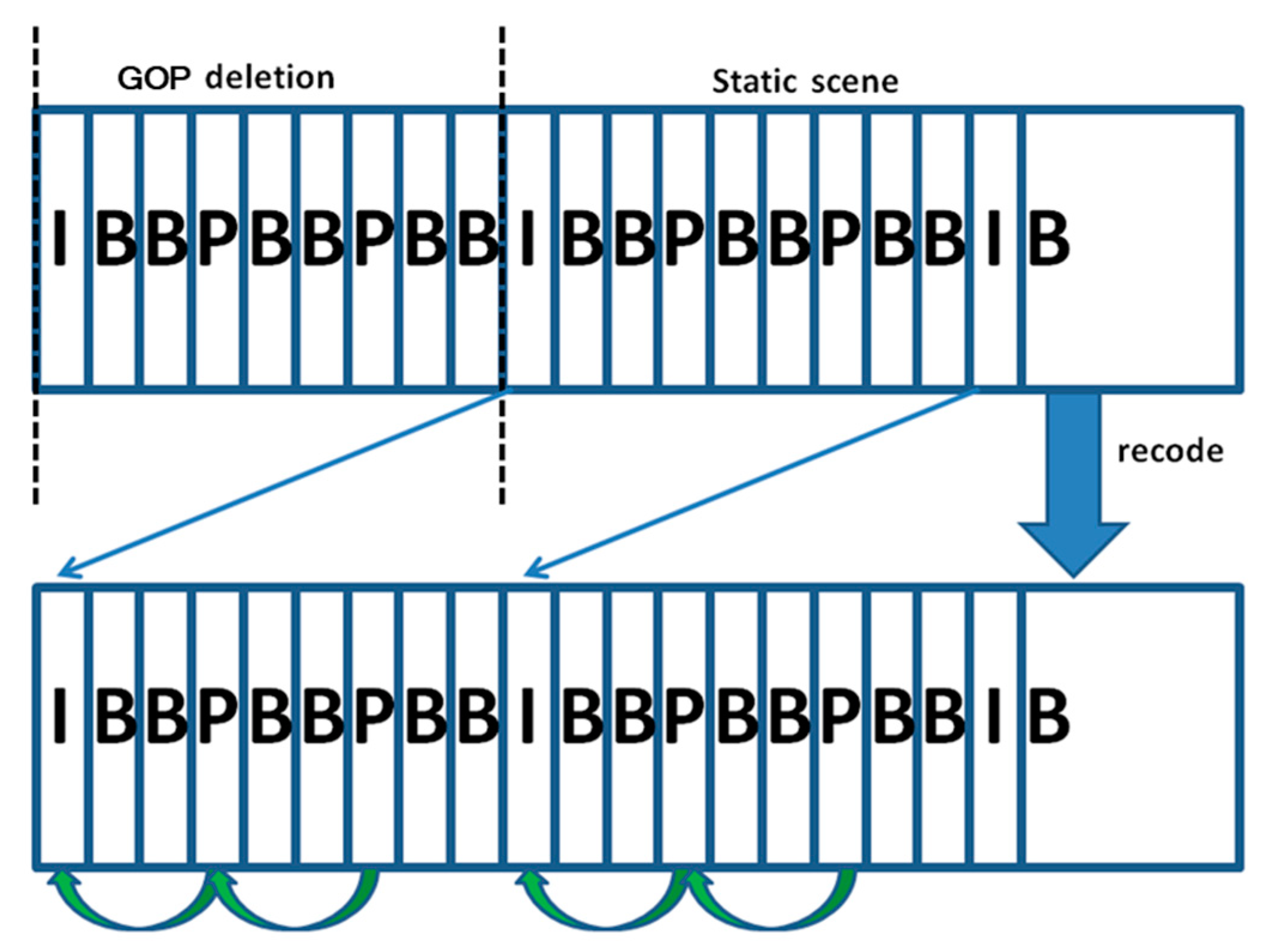
- Integral GOP frame deletion in static scenes is an effective attack against most multiple recoding detection approaches based on Wang et al.’s [35] principle.
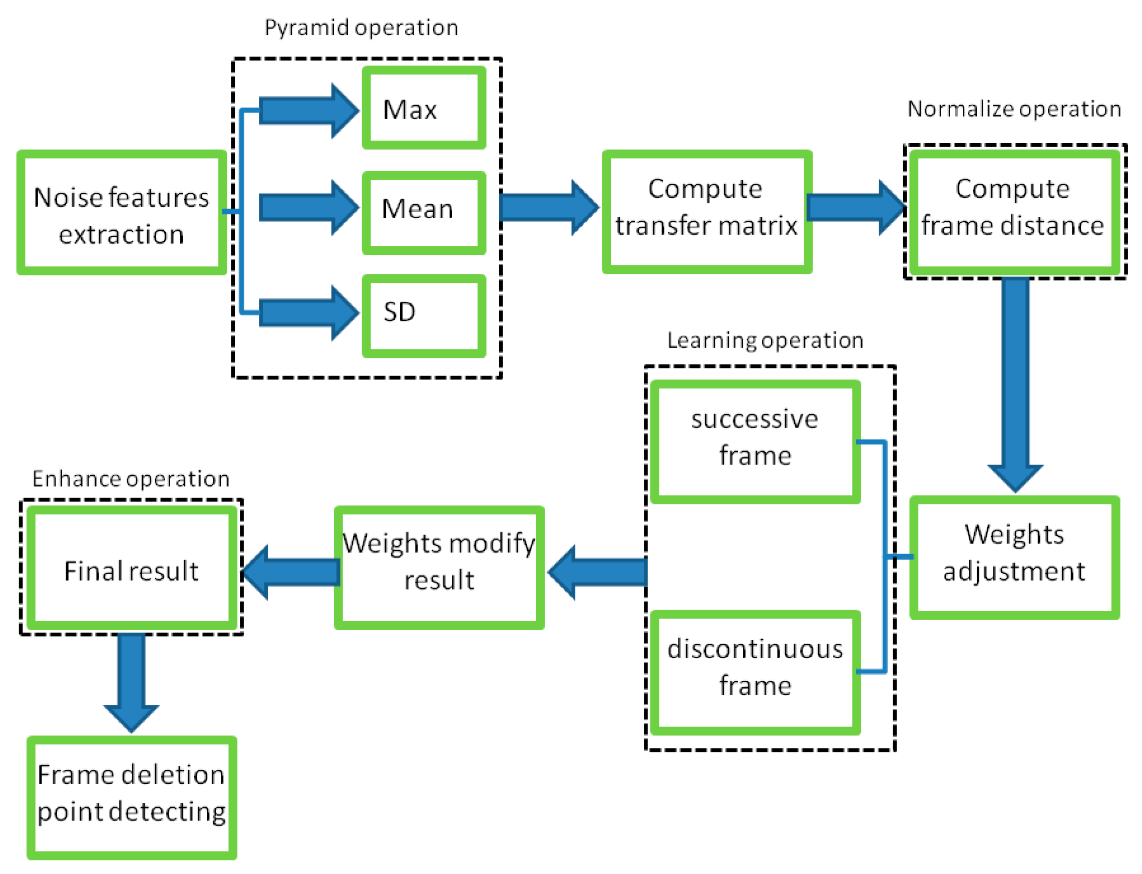
- We propose a novel anti-forensic detection approach to discern forged videos (integral GOP frame deletion in static scenes), using the combination of a pyramid structure and an adaptive weight adjustment module.
- We adopt a pooling operation and pyramid structure to extract noise features, which are available for subsequent analysis with suppressed sensitivity.
- A normalization operation and the combination of successive frame results reduce the influence of variable dimensions and video recording interference.
- Incorporating an adaptive weight adjustment module ensures the algorithm’s universality and fast learning ability with only a single video and diverse environments, thus meeting the practical requirements of forensic science.
- Original videos and visual examples are discussed in the paper, which are intuitive and detailed and display the characteristics of various detection methods.
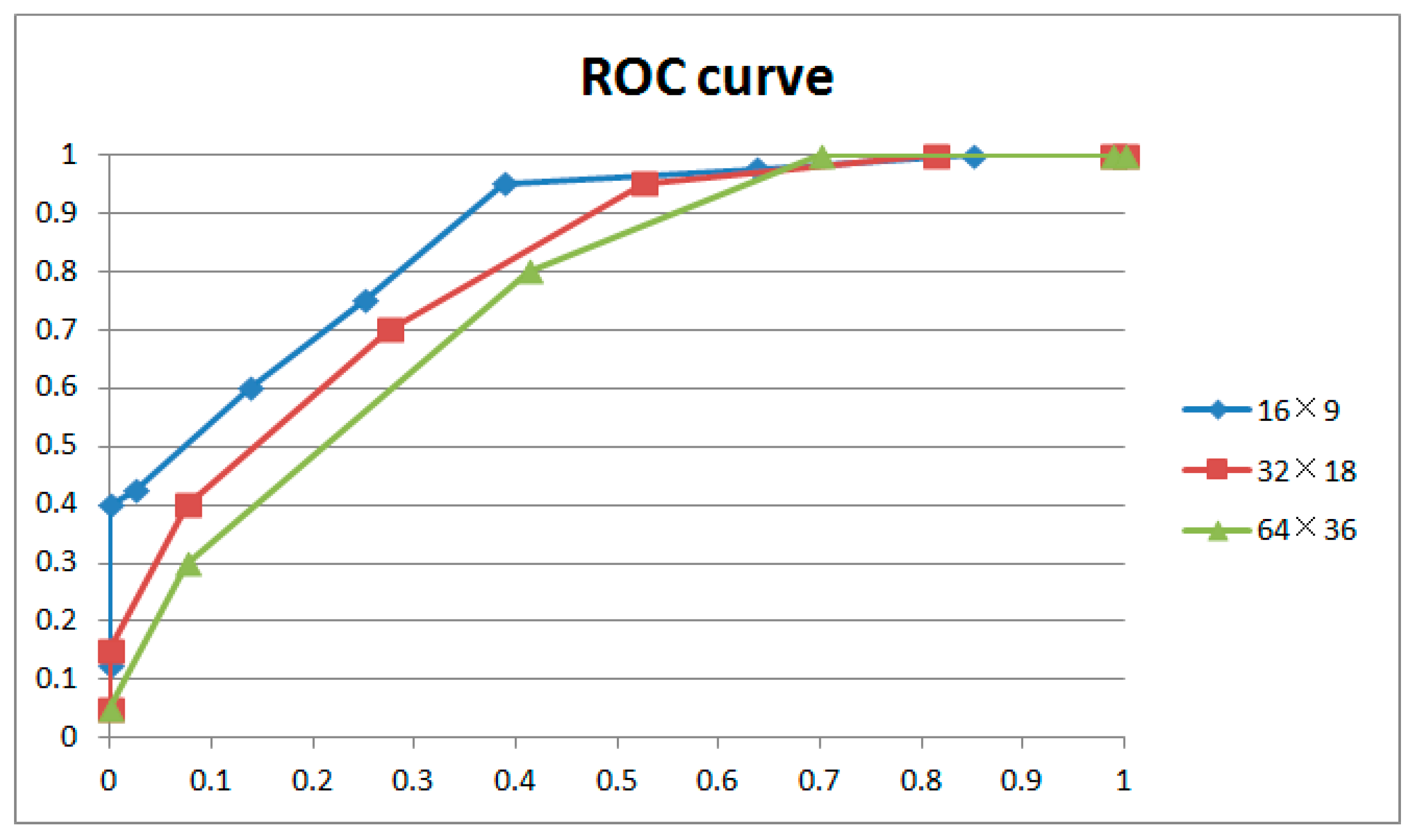
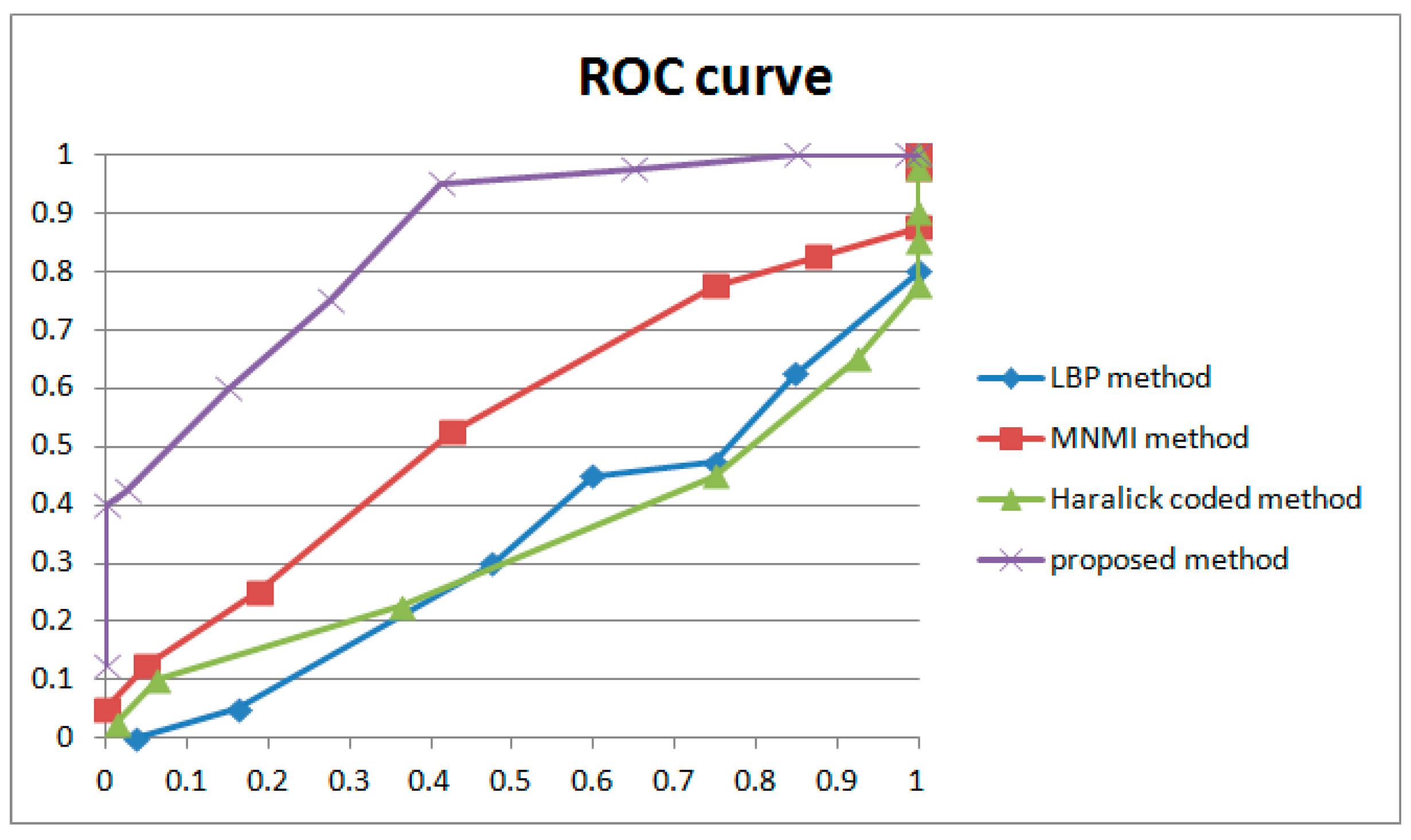
- The receiver operating characteristic (ROC) results demonstrate significant enhancement, particularly in the low false positive rate (FPR), indicating highly improved performance in terms of the forensic principle of no punishment in doubtful cases.
2. Related Works
2.1. Traditional Cue-Based Detection Methods
2.2. Equipment Trace Detection Methods
2.3. Network-Based Detection Methods
2.4. Double Encoding Detection Methods
3. Proposed Approach
3.1. Methods
3.1.1. Noise Extraction
3.1.2. Noise Transfer Matrix Computation
3.1.3. Adjusting Transfer Matrix Weights
4. Experiments
4.1. Dataset
4.2. Coarse Filter
4.3. Parameter Optimization Experiments
4.4. Ablation Experiments
4.5. Comparison Experiments
4.5.1. LBP Method
4.5.2. MNMI Method
4.5.3. Haralick Coded Method
4.5.4. MS-SSIM Method
4.5.5. UFS-MSRC Method
4.5.6. Learning-Based Method Results
4.5.7. Results of Robustness to Anti-Forensics Operation
4.6. Discussion
- (1)
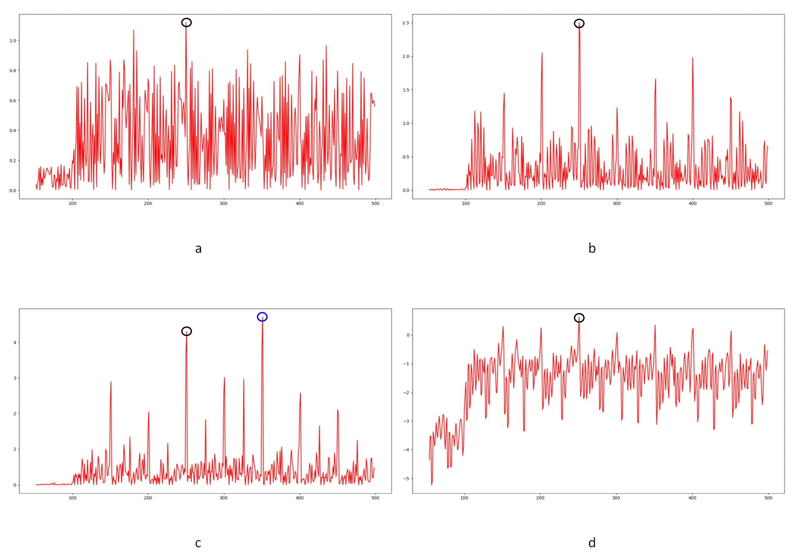
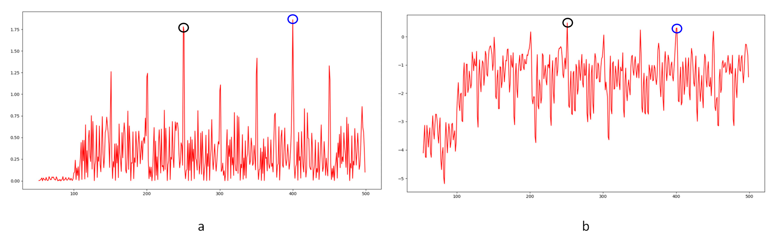
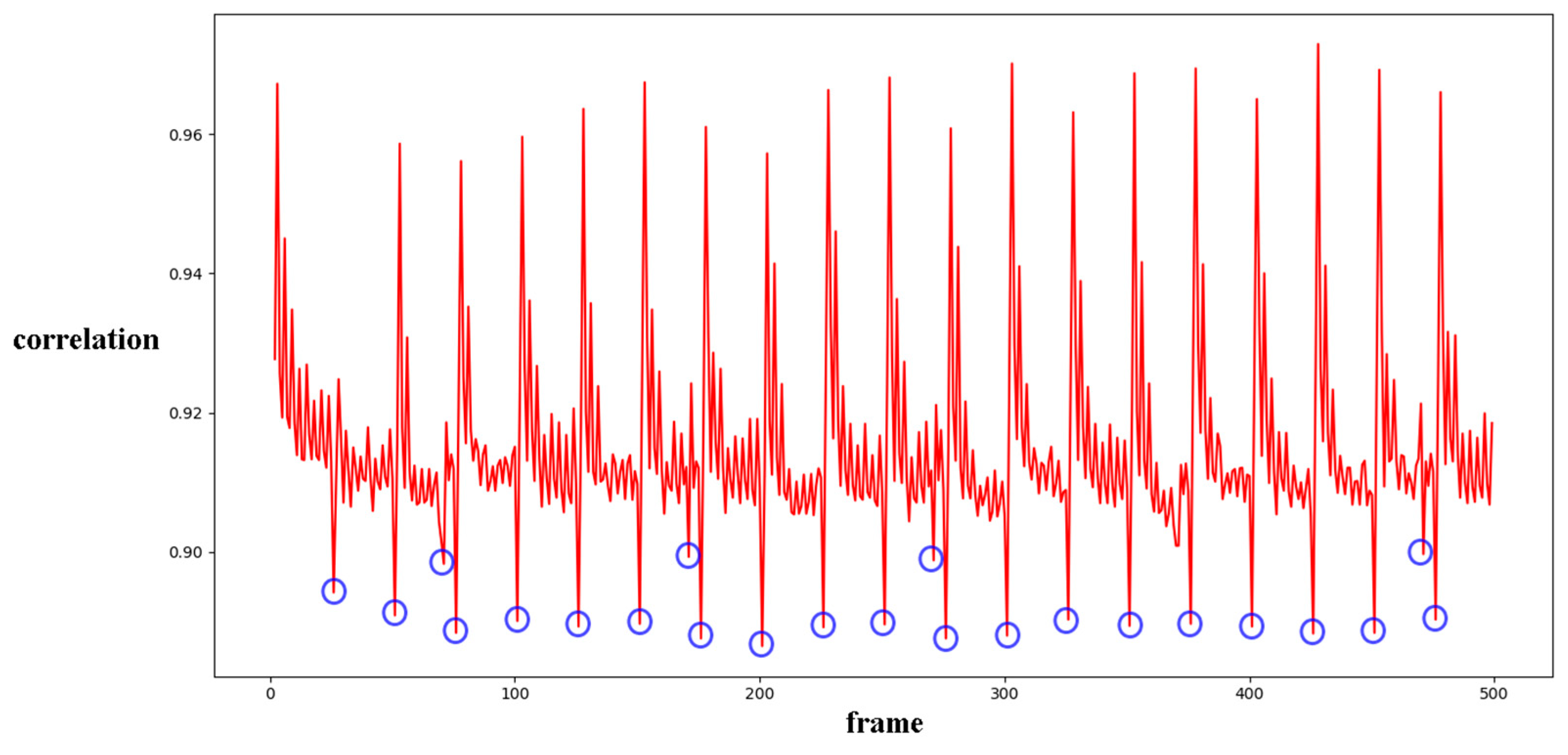
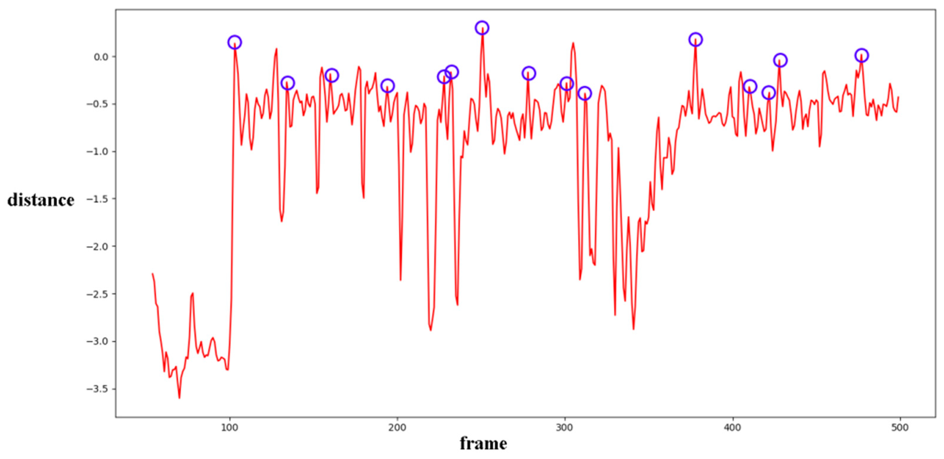
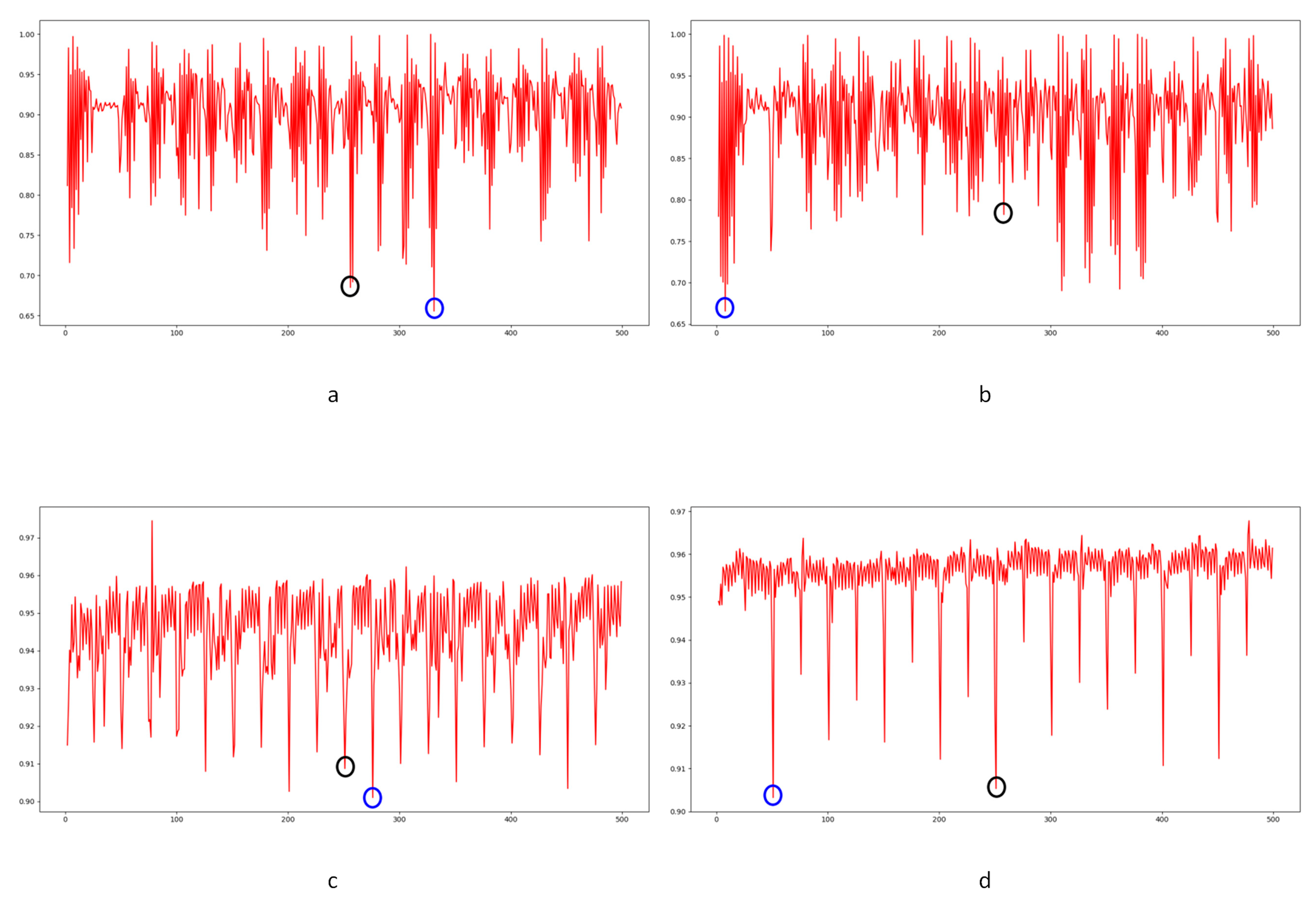
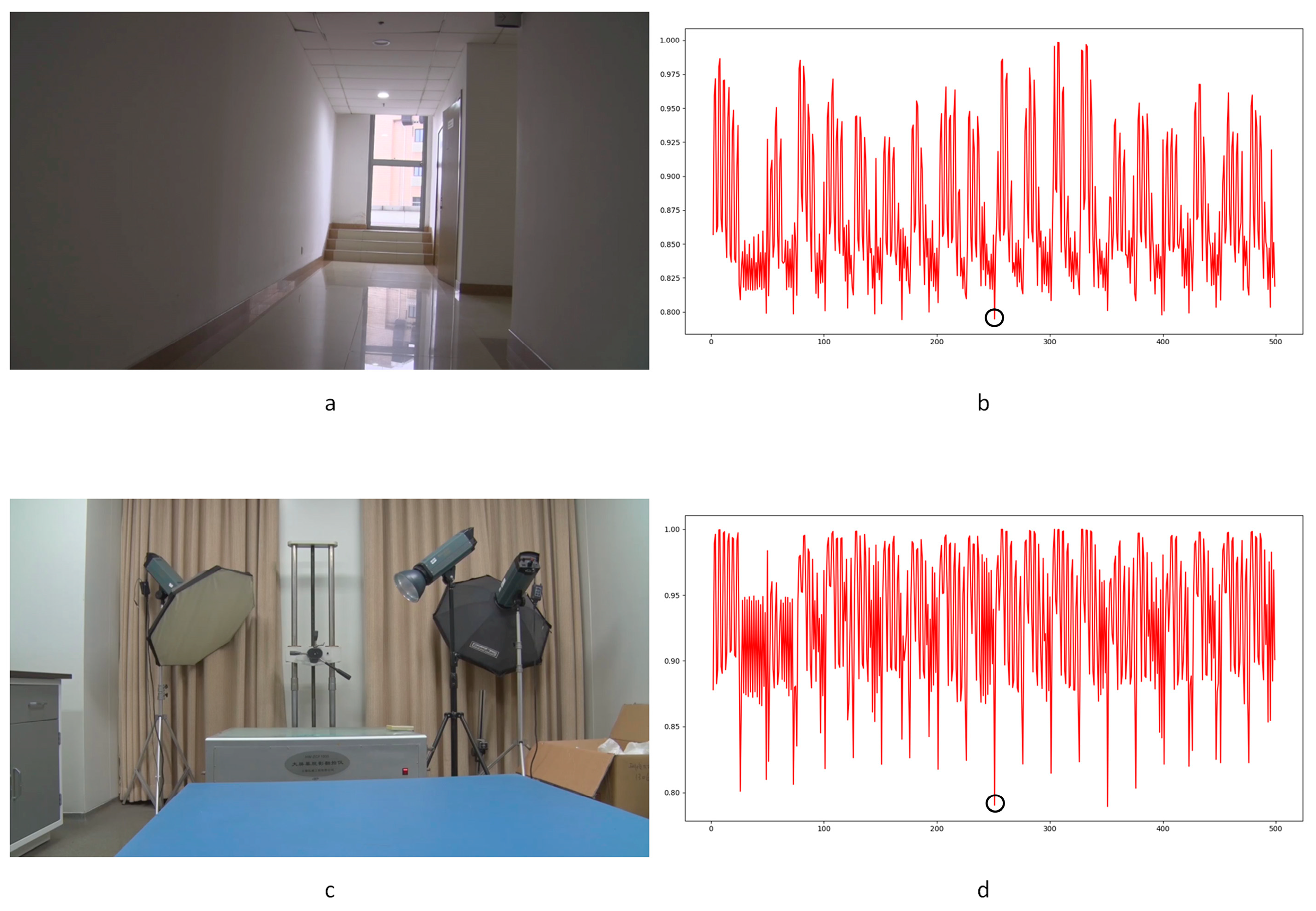
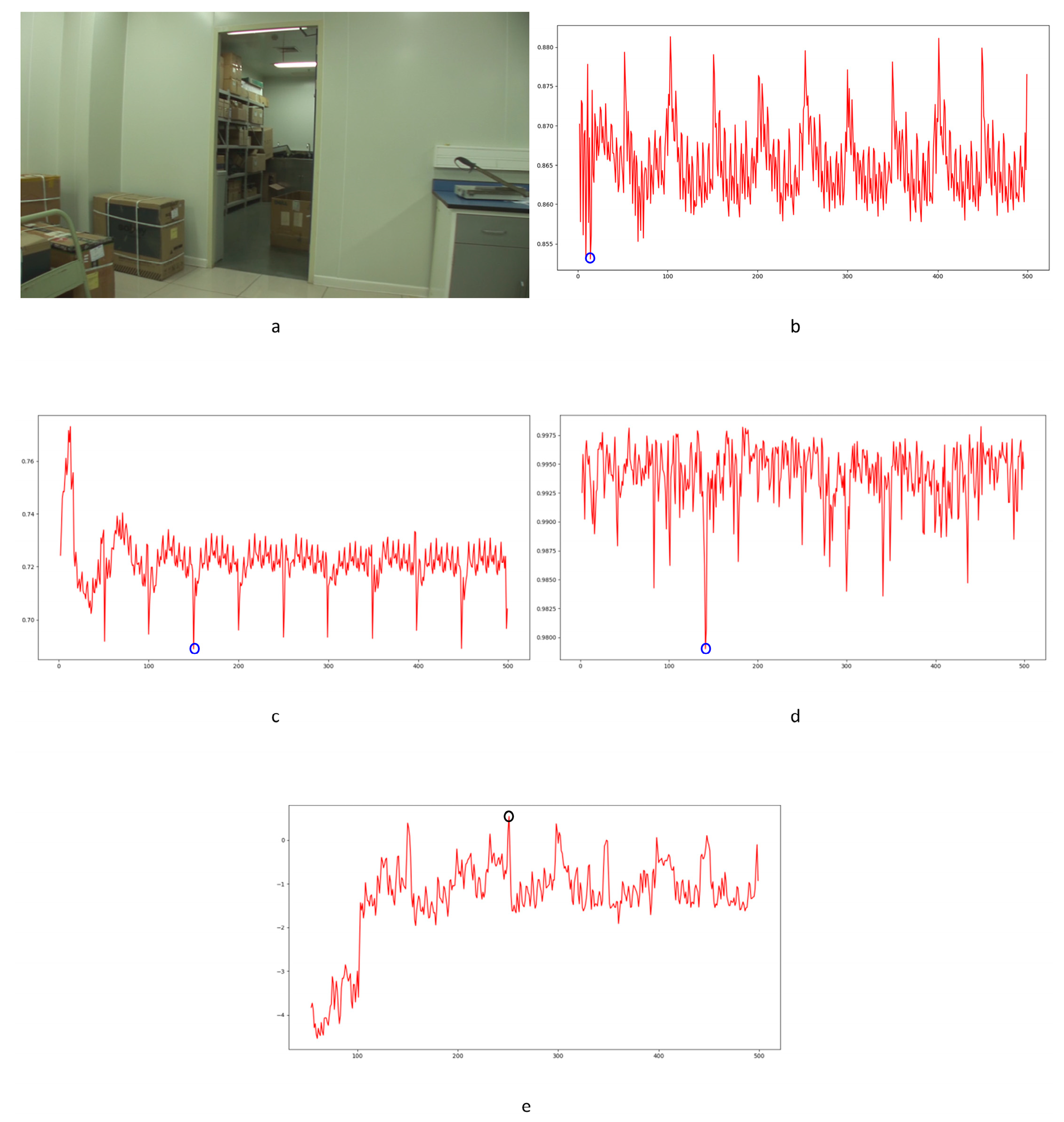
- The LBP, Haralick and MNMI algorithms detect suspected frame deletion points more accurately than random. Even though the ROC curves demonstrate poor performance, there is no doubt that those methods still provide useful information. False positive detection chance represents the dominant quantity in the video. Even considering the periodic effect caused by the GOP structure, the number of possible false positive detection points is dozens of times that of genuine positive detection points. An intuitive example is shown in Figure 12. Points indicated by blue circles indicate participants of the genuine FDP points.
- (2)
- Our approach has improved performance in detecting delicate frame deletion (integral GOP deletion in a static scene) in video compared with other approaches [1,33,34]. From Table 5, we can identify multiple examples of genuine FDPs detected by our approach, while these are ignored by the other approaches. Our approach reaches a TPR of 0.4 with an FPR of 0. However, the compared methods do not reach higher than 0.05. Because of the rigorousness of forensic science, vague clues cannot be accepted as evidence. A high TPR without any dispute can make a vital contribution to court proceedings.
- (3)
- Our approach reduces the possibility of false positive detection caused by various types of interference in video generation. This is a key point in forensic science in terms of verifying the authenticity of a video. In practical work, many novel approaches have been discarded due to the problem of false positive detection. In court, a suspected false positive detection in an entire video could overturn the results of genuine FDP detection. Examples will be given, presenting the characteristics of the proposed approach and comparing the approaches directly.
5. Conclusions
Author Contributions
Funding
Institutional Review Board Statement
Informed Consent Statement
Data Availability Statement
Conflicts of Interest
References
- Zhang, Z.; Hou, J.; Ma, Q.; Li, Z. Efficient video frame insertion and deletion detection based on inconsistency correlations between local binary pattern coded frames. Secur. Commun. Netw. 2015, 8, 311–320. [Google Scholar] [CrossRef]
- Yu, L.; Wang, H.; Han, Q.; Niu, X.; Yiu, S.M.; Fang, J.; Wang, Z. Exposing frame deletion by detecting abrupt changes in video streams. Neurocomputing 2016, 205, 84–91. [Google Scholar] [CrossRef]
- Kumar, V.; Gaur, M. Multiple forgery detection in video using inter-frame correlation distance with dual-threshold. Multimed. Tools Appl. 2022, 81, 43979–43998. [Google Scholar] [CrossRef]
- Sharma, H.; Kanwal, N. Video interframe forgery detection: Classification, technique & new dataset. J. Comput. Secur. 2021, 29, 531–550. [Google Scholar]
- Li, S.; Hou, H. Frame deletion detection based on optical flow orientation variation. IEEE Access 2021, 9, 37196–37209. [Google Scholar] [CrossRef]
- EI-Shafai, W.; Fouda, M.A.; EI-Rabaie, E.S.M.; EI-Salam, N.A. A comprehensive taxonomy on multimedia video forgery detection techniques: Challenges and novel trends. Multimed. Tools Appl. 2024, 83, 4241–4307. [Google Scholar] [CrossRef] [PubMed]
- Milani, S.; Fontani, M.; Bestagini, P.; Barni, M.; Piva, A.; Tagliasacchi, M.; Tubaro, S. An overview on video forensics. APSIPA Trans. Sig. Inf. Process. 2012, 1, e2. [Google Scholar] [CrossRef]
- Long, C.; Smith, E.; Basharat, A.; Hoogs, A. A C3D-based convolutional neural network for frame dropping detection in a single video shot. In Proceedings of the 2017 Conference on Computer Vision and Pattern Recognition Workshops (CVPRW), Honolulu, HI, USA, 21–26 July 2017; pp. 1898–1906. [Google Scholar]
- Long, C.; Basharat, A.; Hoogs, A.; Singh, P.; Farid, H. A coarse-to-fine deep convolutional neural network framework for frame duplication detection and localization in forged videos. IEEE CVPR workshops. 2019, 1-10. In Computer Vision and Pattern Recognition; 2019; pp. 1–10. Available online: https://arxiv.org/abs/1811.10762 (accessed on 16 August 2024).
- Bakas, J.; Naskar, R. A digital forensic technique for inter–frame video forgery detection based on 3D CNN. In Proceedings of the International Conference on Information Systems Security, Bangalore, India, 17–19 December 2018; pp. 304–317. [Google Scholar]
- Yang, Q.; Yu, D.; Zhang, Z.; Yao, Y.; Chen, L. Spatiotemporal trident networks: Detection and localization of object removal tampering in video passive forensics. IEEE Trans. Circuits Syst. Video Technol. 2021, 31, 4131–4144. [Google Scholar] [CrossRef]
- Fadl, S.; Han, Q.; Li, Q. CNN spatiotemporal features and fusion for surveillance video forgery detection. Sig. Process. Image Commun. 2021, 90, 116066. [Google Scholar] [CrossRef]
- Kaur, H.; Jindal, N. Deep convolutional neural network for graphics forgery detection in video. Wirel. Pers. Commun. 2020, 112, 1763–1781. [Google Scholar] [CrossRef]
- Gowda, R.; Pawar, D. Deep learning-based forgery identification and localization in videos. Sig. Image Video Process. 2023, 17, 2185–2192. [Google Scholar] [CrossRef]
- Girish, N.; Nandini, C. Inter-frame video forgery detection using UFS-MSRC algorithm and LSTM network. Int. J. Model. Simul. Sci. Comput. 2023, 14, 2341013. [Google Scholar] [CrossRef]
- Aloraini, M.; Sharifzadeh, M.; Schonfeld, D. Sequential and patch analyses for object removal video forgery detection and localization. IEEE Trans. Circuits Syst. Video Technol. 2020, 31, 917–930. [Google Scholar] [CrossRef]
- Fayyaz, M.A.; Anjum, A.; Ziauddin, S.; Khan, A.; Sarfaraz, A. An improved surveillance video forgery detection technique using sensor pattern noise and correlation of noise residues. Multimed. Tools Appl. 2020, 79, 5767–5788. [Google Scholar] [CrossRef]
- Hsu, C.C.; Hung, T.Y.; Lin, C.W.; Hsu, C.T. Video forgery detection using correlation of noise residue. In Proceedings of the 2008 IEEE 10th Workshop on Multimedia Signal Processing, Cairns, Qld, Australia, 8–10 October 2008; pp. 170–174. [Google Scholar]
- Mandelli, S.; Bestagini, P.; Tubaro, S.; Cozzolion, D.; Verdoliva, L. Blind detection and localization of video temporal splicing exploiting sensor-based footprints. In Proceedings of the 2018 26th European Signal Processing Conference (EUSIPCO), Roma, Italy, 3–7 September 2018; pp. 1362–1366. [Google Scholar]
- Kobayashi, M.; Okabe, T.; Sato, Y. Detecting forgery from static-scene video based on inconsistency in noise level functions. IEEE Trans. Inf. Forensics Secur. 2010, 5, 883–892. [Google Scholar] [CrossRef]
- Bayram, S.; Sencar, H.; Memon, N.; Avcibas, I. Source camera identification based on CFA interpolation. In Proceedings of the IEEE International Conference on Image Processing 2005, Genova, Italy, 14 September 2005; pp. III–69. [Google Scholar]
- Liu, C.; Freeman, W.T.; Szeliski, R.; Kang, S.B. Noise estimation from a single image. In Proceedings of the 2006 IEEE Computer Society Conference on Computer Vision and Pattern Recognition (CVPR 06), New York, NY, USA, 17–22 June 2006; pp. 901–908. [Google Scholar]
- Matsushita, Y.; Lin, S. Radiometric calibration from noise distributions. In Proceedings of the 2007 IEEE Conference on Computer Vision and Pattern Recognition, Minneapolis, MN, USA, 17–22 June 2007; pp. 1–8. [Google Scholar]
- Fadl, S.; Han, Q.; Qiong, L. Exposing video inter-frame forgery via histogram of oriented gradients and motion energy image. Multidimens. Syst. Sig. Process. 2020, 31, 1365–1384. [Google Scholar] [CrossRef]
- Shehnaz; Kaur, M.A. Detection and localization of multiple inter-frame forgeries in digital videos. Multimed. Tools Appl. 2024, 83, 1–33. [Google Scholar] [CrossRef]
- Wang, Q.; Li, Z.; Zhang, Z.; Ma, Q.A. Video inter-frame forgery identification based on consistency of correlation coefficients of gray values. J. Comput. Commun. 2014, 2, 51–57. [Google Scholar] [CrossRef]
- Wang, Q.; Li, Z.; Zhang, Z.; Ma, Q.A. Video inter-frame forgery identification based on optical flow consistency. Sens. Transducers 2014, 166, 229–234. [Google Scholar]
- He, K.; Zhang, X.; Ren, S.; Sun, J. Deep Residual learning for image recognition. In Proceedings of the 2017 IEEE International Symposium on Technologies for Homeland Security (HST), Las Vegas, NV, USA, 27–30 June 2017; pp. 770–778. [Google Scholar]
- Wan, Q.; Panetta, K.; Agaian, S. A video forensic technique for detecting frame integrity using human visual system-inspired measure. In Proceedings of the IEEE Conference on Computer Vision and Pattern Recognition (CVPR), Waltham, MA, USA, 25–26 April 2016; pp. 1–6. [Google Scholar]
- Jing, Z.; Su, Y.; Zhang, M. Exposing digital video forgery by ghost shadow artifact. In Proceedings of the First ACM Workshop on Multimedia in Forensics, Tianjin, China, 23 October 2009; pp. 49–54. [Google Scholar]
- Feng, C.; Xu, Z.; Jia, S.; Zhang, W.; Xu, Y. Motion-adaptive frame deletion detection for digital video forensics. IEEE Trans. Circuits Syst. Video Technol. 2016, 27, 2543–2554. [Google Scholar] [CrossRef]
- Kingra, S.; Aggarwal, N.; Singh, R.W. Inter-frame forgery detection in H.264 videos using motion and brightness gradients. Multimed. Tools Appl. 2017, 76, 25767–25786. [Google Scholar] [CrossRef]
- Zhao, Y.; Pang, T.; Liang, X.; Li, Z. Frame-deletion detection for static-background video based on multi-scale mutual information. In Proceedings of the International Conference on Cloud Computing and Security (ICCCS 2017), Nanjing, China, 16–18 June 2017; pp. 371–384. [Google Scholar]
- Bakas, J.; Naskar, R.; Dixit, R. Detection and localization of inter-frame video forgeries based on inconsistency in correlation distribution between Haralick coded frames. Multimed. Tools Appl. 2019, 78, 4905–4935. [Google Scholar] [CrossRef]
- Wang, W.; Fraid, H. Exposing digital forgeries in video by detecting double MPEG compression. In Proceedings of the 8th Workshop on Multimedia and Security, Geneva, Switzerland, 26–27 September 2006; pp. 37–47. [Google Scholar]
- Stamm, M.C.; Lin, W.S.; Liu, K.J.R. Temporal forensics and anti-forensics for motion compensated video. IEEE Trans. Inf. Forensics Secur. 2012, 7, 1315–1329. [Google Scholar] [CrossRef]
- Gironi, A.; Fontani, M.; Bianchi, T.; Piva, A.; Barni, M. A video forensic technique for detecting frame deletion and insertion. In Proceedings of the 2014 IEEE International Conference on Acoustics, Speech, and Signal Processing (ICASSP), Florence, Italy, 4–9 May 2014; pp. 6226–6230. [Google Scholar]
- Jiang, X.; Wang, W.; Sun, T.; Shi, Y.Q.; Shilin, W. Detection of double compression in MPEG-4 videos based on Markov statistics. IEEE Sig. Process. Lett. 2013, 20, 447–450. [Google Scholar] [CrossRef]
- Shanableh, T. Detection of frame deletion for digital video forensics. Digit. Investig. 2013, 10, 350–360. [Google Scholar] [CrossRef]
- Liu, H.; Li, S.; Bian, S. Detecting frame deletion in H. 264 video. In Proceedings of the International Conference on Information Security Practice and Experience (ISPEC 2014), Fuzhou, China, 5–8 May 2014; pp. 262–270. [Google Scholar]
- Vazquez-Padin, D.; Fontani, M.; Bianchi, T.; Comesana, P.; Piva, A.; Barni, M. Detection of video double encoding with GOP size estimation. In Proceedings of the 2012 IEEE International Workshop on Information Forensics and Security (WIFS), Costa Adeje, Spain, 2–5 December 2012; pp. 151–156. [Google Scholar]
- Hong, J.H.; Yang, Y.; Oh, B.T. Detection of frame deletion in HEVC-Coded video in the compressed domain. Digit. Investig. 2019, 30, 23–31. [Google Scholar] [CrossRef]
- Singh, R.D.; Aggarwal, D. Detection of re-compression, transcoding and frame-deletion for digital video authentication. In Proceedings of the 2015 2nd International Conference on Recent Advances in Engineering & Computational Sciences (RAECS), Chandigarh, India, 21–22 December 2015; pp. 1–6. [Google Scholar]
- Bakas, J.; Naskar, R.; Bakshi, S. Detection and localization of inter-frame forgeries in videos based on macroblock variation and motion vector analysis. Comp. Electr. Eng. 2021, 89, 106929. [Google Scholar] [CrossRef]
- Shekar, B.H.; Abraham, W.; Pilar, B. A simple difference based inter frame video forgery detection and localization. In Proceedings of the International Conference on Soft Computing and its Engineering Applications (icSoftComp 2023), Changa, Anand, India, 7–9 December 2023; pp. 3–15. [Google Scholar]
- Wang, W.; Jiang, X.; Wang, S.; Wan, M.; Sun, T. Identifying video forgery process using optical flow. In Proceedings of the International WorkshopDigital-Forensics and Watermarking (IWDW 2013), Auckland, New Zealand, 1–4 October 2013; pp. 244–257. [Google Scholar]
- Dar, Y.; Bruckstein, A.M. Motion-compensated coding and frame rate up-conversion: Models and analysis. IEEE Trans. Image Process. 2015, 24, 2051–2066. [Google Scholar] [CrossRef] [PubMed]
- Yao, H.; Ni, R.; Zhao, Y. An approach to detect video frame deletion under anti-forensics. J. Real-Time Image Process. 2019, 16, 751–764. [Google Scholar] [CrossRef]
- Reibman, A.R.; Poole, D. Characterizing packet-loss impairments in compressed video. In Proceedings of the 2007 IEEE International Conference on Image Processing, San Antonio, TX, USA, 16 September 2007–19 October 2007; pp. 77–80. [Google Scholar]
- Reibman, A.R.; Vaishampayan, V.A.; Sermadevi, Y. Quality monitoring of video over a packet network. IEEE Trans. Multimed. 2004, 6, 327–334. [Google Scholar] [CrossRef]
- Li, H.; Bao, Q.; Deng, N. Detection of video continuity based on noise Markov transfer matrix. J. Crim. Investig. Police Univ. China 2019, 149, 125–128. [Google Scholar]
- Chen, J.; Kang, X.; Liu, Y.; Wang, Z.J. Median filtering forensics based on convolutional neural networks. IEEE Sig. Process. Lett. 2015, 22, 1849–1853. [Google Scholar] [CrossRef]
- Kirchner, M.; Rohme, R. Hiding traces of resampling in digital images. IEEE Trans. Inf. Forensics Secur. 2008, 3, 582–592. [Google Scholar] [CrossRef]
- Pawar, S.; Pradhan, G.; Goswami, B.; Bhutad, S. Identifying Fake Images Through CNN Based Classification Using FIDAC. In Proceedings of the 2022 International Conference on Intelligent Controller and Computing for Smart Power (ICICCSP), Hyderabad, India, 21–23 July 2022; pp. 1–6. [Google Scholar]
- Lin, T.; Goyal, P.; Girshick, R.; He, K.; Dollar, P. Focal loss for dense object detection. In Proceedings of the 2017 IEEE International Conference on Computer Vision (ICCV), Venice, Italy, 22–29 October 2017; pp. 2999–3007. [Google Scholar]
- Patel, J.; Sheth, R. An optimized convolution neural network based inter-frame forgery detection model—A multi-feature extraction framework. ICTACT J. Image Video Process. 2021, 12, 2570–2581. [Google Scholar]
- Paing, S.; Htun, Y. An unsupervised learning algorithm based deletion of Inter-frame forgery detection system. In Proceedings of the 2023 International Conference on Research Methodologies in Knowledge Management, Artificial Intelligence and Telecommunication Engineering (RMKMATE), Chennai, India, 1–2 November 2023; pp. 1–4. [Google Scholar]
- Chen, C.; Shi, Y.Q.; Su, W. A machine learning based scheme for double JPEG compression detection. In Proceedings of the 2008 19th International Conference on Pattern Recognition, Tampa, FL, USA, 8–11 December 2008; pp. 1–4. [Google Scholar]
- Thing, V.L.L.; Chen, Y.; Cheh, C. An improved double compression detection method for JPEG image forensics. In Proceedings of the 2012 IEEE International Symposium on Multimedia, Irvine, CA, USA, 10–12 December 2012; pp. 290–297. [Google Scholar]
- Fisher, R.A. The use of multiple measurements in taxonomic problems. Ann. Eugen. 1936, 7, 179–188. [Google Scholar] [CrossRef]
- Su, Y.; Nie, W.; Zhang, C. A frame tampering detection algorithm for MPEG videos. In Proceedings of the 2011 6th IEEE Joint International Information Technology and Artificial Intelligence Conference, Chongqing, China, 20–22 August 2011; pp. 461–464. [Google Scholar]
- Wu, Y.; Jiang, X.; Sun, T.; Wang, W. Exposing video inter-frame forgery based on velocity field consistency. In Proceedings of the 2014 IEEE International Conference on Acoustics, Speech, and Signal Processing (ICASSP), Florence, Italy, 4–9 May 2014; pp. 2674–2678. [Google Scholar]
- Yang, J.; Zhou, K.; Li, Y.; Liu, Z. Generalized out-of-distribution detection: A survey. Int. J. Comput. Vis. 2024, 1–28. [Google Scholar] [CrossRef]
- Zhu, L.; Yang, Y.; Gu, Q.; Wang, X.; Zhou, C.; Ye, N. CRoFT: Robust fine-tuning with concurrent optimization for OOD generalization and open-set OOD detection. arXiv 2024, arXiv:2405.16417. [Google Scholar]


| Scene | 16 × 9 True Positive | 16 × 9 False Positive | 32 × 18 True Positive | 32 × 18 False Positive | 64 × 36 True Positive | 64 × 36 False Positive |
|---|---|---|---|---|---|---|
| 1 | / | 1.5 | / | 1.5 | / | 1.5 |
| 2 | / | 2.5 | / | 2 | / | 2 |
| 3 | / | 2.5 | / | 2.5 | / | 2.5 |
| 4 | / | 3 | / | 3 | / | 2.5 |
| 5 | / | 2 | / | 2.5 | / | 2 |
| 6 | / | 2 | / | 2 | / | 2 |
| 7 | / | 2 | / | 2 | / | 2 |
| 8 | / | 2 | / | 2.5 | / | 2.5 |
| 9 | / | 2 | / | 2.5 | / | 2 |
| 10 | / | 3 | / | 2.5 | / | 2.5 |
| 11 | / | 2.5 | / | 2 | / | 2 |
| 12 | / | 3 | / | 3 | / | 2.5 |
| 13 | / | 2 | / | 2 | / | 2 |
| 14 | / | 2 | / | 2.5 | / | 2.5 |
| 15 | / | 2 | / | 2 | / | 2 |
| 16 | / | 2.5 | / | 2 | / | 2 |
| 17 | / | 2.5 | / | 2 | / | 2 |
| 18 | / | 2 | / | 2 | / | 2 |
| 19 | / | 2.5 | / | 2.5 | / | 2.5 |
| 20 | / | 3 | / | 2.5 | / | 2.5 |
| 21 | 4 | 2.5 | 3 | 2.5 | 2.5 | 2 |
| 22 | 3 | 3 | 3 | 3 | 3 | 3 |
| 23 | 4 | 3.5 | 3 | 2.5 | 2.5 | 2.5 |
| 24 | 3.5 | 3.5 | 3 | 2.5 | 2.5 | 2.5 |
| 25 | 4.5 | 3.5 | 3 | 3 | 3 | 3 |
| 26 | 3.5 | 2.5 | 2.5 | 2 | 2.5 | 2 |
| 27 | 5 | 3.5 | 3.5 | 3 | 3 | 2.5 |
| 28 | 3.5 | 3 | 3.5 | 3 | 3 | 3 |
| 29 | 4 | 4.5 | 3.5 | 3.5 | 3 | 3 |
| 30 | 4 | 4.5 | 3.5 | 3.5 | 3 | 3 |
| 31 | 6 | 4 | 4.5 | 3 | 3 | 3 |
| 32 | 5 | 3.5 | 4 | 3.5 | 3.5 | 3 |
| 33 | 5.5 | 3 | 4 | 3 | 3 | 3 |
| 34 | 5.5 | 3.5 | 4 | 3.5 | 3 | 3 |
| 35 | 4.5 | 4.5 | 4 | 4 | 3.5 | 3.5 |
| 36 | 3.5 | 3.5 | 3 | 3 | 2.5 | 2.5 |
| 37 | 4.5 | 4.5 | 4 | 4 | 3 | 3 |
| 38 | 4.5 | 3.5 | 3.5 | 3 | 3 | 3 |
| 39 | 4 | 3 | 3 | 3 | 3 | 3 |
| 40 | 3.5 | 5 | 3.5 | 3.5 | 3 | 3 |
| 41 | / | 2 | / | 2 | / | 2 |
| 42 | / | 2 | / | 2 | / | 2 |
| 43 | / | 2.5 | / | 2.5 | / | 2.5 |
| 44 | / | 2.5 | / | 2.5 | / | 2 |
| 45 | / | 2.5 | / | 2.5 | / | 2 |
| 46 | / | 2.5 | / | 2.5 | / | 2 |
| 47 | / | 3 | / | 2.5 | / | 2.5 |
| 48 | / | 3 | / | 2.5 | / | 2.5 |
| 49 | / | 2.5 | / | 2.5 | / | 2 |
| 50 | / | 2.5 | / | 2.5 | / | 2 |
| 51 | / | 3 | / | 2 | / | 2 |
| 52 | / | 3 | / | 3 | / | 2.5 |
| 53 | / | 4 | / | 2.5 | / | 2.5 |
| 54 | / | 3.5 | / | 3 | / | 2.5 |
| 55 | / | 2.5 | / | 2.5 | / | 2.5 |
| 56 | / | 3 | / | 3 | / | 3 |
| 57 | / | 4.5 | / | 3.5 | / | 3 |
| 58 | / | 2.5 | / | 2 | / | 2 |
| 59 | / | 3 | / | 2.5 | / | 2 |
| 60 | / | 2.5 | / | 2.5 | / | 2.5 |
| 61 | 5.5 | 4 | 4 | 4 | 3.5 | 3 |
| 62 | 5 | 4.5 | 3.5 | 3.5 | 3 | 3 |
| 63 | 5 | 5 | 3.5 | 3.5 | 3 | 3 |
| 64 | 5.5 | 4.5 | 5 | 4 | 3.5 | 3.5 |
| 65 | 6 | 4 | 4 | 3.5 | 4 | 3 |
| 66 | 4.5 | 3 | 3.5 | 3 | 3 | 3 |
| 67 | 5.5 | 4 | 4 | 3.5 | 3.5 | 3.5 |
| 68 | 5 | 3 | 3.5 | 3 | 3 | 2.5 |
| 69 | 4 | 3 | 3 | 3 | 3 | 3 |
| 70 | 4.5 | 3 | 3.5 | 3.5 | 3.5 | 3.5 |
| 71 | 3.5 | 3.5 | 3 | 3 | 2.5 | 2.5 |
| 72 | 6 | 4.5 | 4.5 | 4 | 3.5 | 3.5 |
| 73 | 6 | 4 | 4.5 | 3.5 | 3.5 | 3 |
| 74 | 4.5 | 4.5 | 4 | 4 | 3.5 | 3.5 |
| 75 | 3.5 | 3 | 3.5 | 3 | 3 | 3 |
| 76 | 3.5 | 3 | 3 | 3 | 2.5 | 2.5 |
| 77 | 2.5 | 4 | 2.5 | 3.5 | 2.5 | 3 |
| 78 | 6 | 3.5 | 5 | 3.5 | 4 | 3 |
| 79 | 5.5 | 4 | 4 | 3.5 | 3.5 | 3 |
| 80 | 5 | 4 | 4.5 | 3.5 | 3 | 3 |
| Scene | 0.75 True Positive | 0.75 False Positive | 1 True Positive | 1 False Positive | 1.25 True Positive | 1.25 False Positive |
|---|---|---|---|---|---|---|
| 1 | / | 2 | / | 1.5 | / | 2.5 |
| 2 | / | 2.5 | / | 2.5 | / | 2.5 |
| 3 | / | 2.5 | / | 2.5 | / | 3 |
| 4 | / | 2.5 | / | 3 | / | 3 |
| 5 | / | 2.5 | / | 2 | / | 2.5 |
| 6 | / | 2 | / | 2 | / | 2.5 |
| 7 | / | 2 | / | 2 | / | 3 |
| 8 | / | 2.5 | / | 2 | / | 2.5 |
| 9 | / | 2.5 | / | 2 | / | 3 |
| 10 | / | 2.5 | / | 3 | / | 2.5 |
| 11 | / | 3.5 | / | 2.5 | / | 3 |
| 12 | / | 3 | / | 3 | / | 3 |
| 13 | / | 2.5 | / | 2 | / | 3 |
| 14 | / | 2.5 | / | 2 | / | 3 |
| 15 | / | 2 | / | 2 | / | 2.5 |
| 16 | / | 2.5 | / | 2.5 | / | 2.5 |
| 17 | / | 2.5 | / | 2.5 | / | 3 |
| 18 | / | 2 | / | 2 | / | 3 |
| 19 | / | 2.5 | / | 2.5 | / | 2.5 |
| 20 | / | 2.5 | / | 3 | / | 2.5 |
| 21 | 3.5 | 2.5 | 4 | 2.5 | 3.5 | 2.5 |
| 22 | 3 | 2.5 | 3 | 3 | 3.5 | 2.5 |
| 23 | 3.5 | 3.5 | 4 | 3.5 | 3 | 3 |
| 24 | 3.5 | 3.5 | 3.5 | 3.5 | 4 | 3.5 |
| 25 | 3.5 | 3 | 4.5 | 3.5 | 3 | 3 |
| 26 | 3.5 | 3 | 3.5 | 2.5 | 3 | 3.5 |
| 27 | 4.5 | 3.5 | 5 | 3.5 | 3.5 | 4 |
| 28 | 3.5 | 3 | 3.5 | 3 | 3.5 | 3 |
| 29 | 4 | 4 | 4 | 4.5 | 3 | 3 |
| 30 | 4 | 4 | 4 | 4.5 | 3.5 | 4.5 |
| 31 | 5 | 4 | 6 | 4 | 4.5 | 4 |
| 32 | 5 | 4 | 5 | 3.5 | 4.5 | 4 |
| 33 | 4 | 2.5 | 5.5 | 3 | 3 | 3.5 |
| 34 | 5 | 3 | 5.5 | 3.5 | 3.5 | 3 |
| 35 | 4 | 4 | 4.5 | 4.5 | 4.5 | 4 |
| 36 | 3.5 | 3.5 | 3.5 | 3.5 | 3 | 3 |
| 37 | 4.5 | 4 | 4.5 | 4.5 | 3.5 | 4 |
| 38 | 4.5 | 3.5 | 4.5 | 3.5 | 4.5 | 3.5 |
| 39 | 3 | 2.5 | 4 | 3 | 3.5 | 3 |
| 40 | 3.5 | 5 | 3.5 | 5 | 4 | 5 |
| 41 | / | 2.5 | / | 2 | / | 3 |
| 42 | / | 3 | / | 2 | / | 3 |
| 43 | / | 2.5 | / | 2.5 | / | 2.5 |
| 44 | / | 2.5 | / | 2.5 | / | 2.5 |
| 45 | / | 3 | / | 2.5 | / | 3 |
| 46 | / | 3 | / | 2.5 | / | 3.5 |
| 47 | / | 3 | / | 3 | / | 3.5 |
| 48 | / | 2.5 | / | 3 | / | 2.5 |
| 49 | / | 2.5 | / | 2.5 | / | 3 |
| 50 | / | 3.5 | / | 2.5 | / | 3 |
| 51 | / | 3 | / | 3 | / | 3 |
| 52 | / | 3.5 | / | 3 | / | 3.5 |
| 53 | / | 4 | / | 4 | / | 3.5 |
| 54 | / | 3.5 | / | 3.5 | / | 3.5 |
| 55 | / | 2.5 | / | 2.5 | / | 2.5 |
| 56 | / | 3 | / | 3 | / | 3.5 |
| 57 | / | 4 | / | 4.5 | / | 4.5 |
| 58 | / | 2.5 | / | 2.5 | / | 2 |
| 59 | / | 3 | / | 3 | / | 3 |
| 60 | / | 2.5 | / | 2.5 | / | 3 |
| 61 | 4.5 | 4 | 5.5 | 4 | 4.5 | 4 |
| 62 | 4.5 | 4 | 5 | 4.5 | 4.5 | 4 |
| 63 | 5 | 5 | 5 | 5 | 4.5 | 4.5 |
| 64 | 5 | 4.5 | 5.5 | 4.5 | 5 | 4.5 |
| 65 | 5.5 | 4.5 | 6 | 4 | 6 | 5 |
| 66 | 4.5 | 3 | 4.5 | 3 | 4.5 | 3 |
| 67 | 4.5 | 3.5 | 5.5 | 4 | 3.5 | 3 |
| 68 | 4 | 3 | 5 | 3 | 3.5 | 3 |
| 69 | 3.5 | 3 | 4 | 3 | 4 | 3.5 |
| 70 | 4 | 3 | 4.5 | 3 | 3.5 | 3.5 |
| 71 | 3.5 | 3.5 | 3.5 | 3.5 | 4 | 4 |
| 72 | 5.5 | 4.5 | 6 | 4.5 | 4 | 4 |
| 73 | 5 | 4 | 6 | 4 | 4.5 | 4 |
| 74 | 4.5 | 4 | 4.5 | 4.5 | 4 | 3.5 |
| 75 | 3.5 | 3.5 | 3.5 | 3 | 4 | 4.5 |
| 76 | 3 | 3 | 3.5 | 3 | 3.5 | 3 |
| 77 | 2.5 | 4 | 2.5 | 4 | 3 | 4 |
| 78 | 5 | 3.5 | 6 | 3.5 | 3.5 | 3.5 |
| 79 | 4.5 | 3.5 | 5.5 | 4 | 4 | 4 |
| 80 | 4 | 4 | 5 | 4 | 4.5 | 4 |
| Scene | = 2 True Positive | = 2 False Positive | = 3 True Positive | = 3 False Positive | = 4 True Positive | = 4 False Positive |
|---|---|---|---|---|---|---|
| 1 | / | 2 | / | 1.5 | / | 2.5 |
| 2 | / | 2.5 | / | 2.5 | / | 3 |
| 3 | / | 2.5 | / | 2.5 | / | 2.5 |
| 4 | / | 3 | / | 3 | / | 3 |
| 5 | / | 2.5 | / | 2 | / | 2.5 |
| 6 | / | 2 | / | 2 | / | 2.5 |
| 7 | / | 2 | / | 2 | / | 2.5 |
| 8 | / | 2.5 | / | 2 | / | 2.5 |
| 9 | / | 2 | / | 2 | / | 2.5 |
| 10 | / | 3 | / | 3 | / | 2.5 |
| 11 | / | 3 | / | 2.5 | / | 3.5 |
| 12 | / | 3 | / | 3 | / | 3 |
| 13 | / | 2.5 | / | 2 | / | 3 |
| 14 | / | 2 | / | 2 | / | 2.5 |
| 15 | / | 2 | / | 2 | / | 2 |
| 16 | / | 2.5 | / | 2.5 | / | 2.5 |
| 17 | / | 2.5 | / | 2.5 | / | 3 |
| 18 | / | 2.5 | / | 2 | / | 2.5 |
| 19 | / | 2.5 | / | 2.5 | / | 2.5 |
| 20 | / | 3 | / | 3 | / | 3 |
| 21 | 3.5 | 2.5 | 4 | 2.5 | 4 | 3.5 |
| 22 | 3 | 3 | 3 | 3 | 3.5 | 3.5 |
| 23 | 3.5 | 3 | 4 | 3.5 | 3 | 3.5 |
| 24 | 3.5 | 3.5 | 3.5 | 3.5 | 4 | 3.5 |
| 25 | 3.5 | 3.5 | 4.5 | 3.5 | 3.5 | 3 |
| 26 | 3 | 2.5 | 3.5 | 2.5 | 3 | 3 |
| 27 | 4 | 3.5 | 5 | 3.5 | 4.5 | 4 |
| 28 | 3.5 | 3 | 3.5 | 3 | 3.5 | 4 |
| 29 | 4 | 3 | 4 | 4.5 | 3.5 | 5 |
| 30 | 4 | 4 | 4 | 4.5 | 4 | 4.5 |
| 31 | 4.5 | 3.5 | 6 | 4 | 5 | 4.5 |
| 32 | 4.5 | 3.5 | 5 | 3.5 | 4.5 | 4 |
| 33 | 4.5 | 3 | 5.5 | 3 | 5.5 | 4 |
| 34 | 5 | 3 | 5.5 | 3.5 | 4.5 | 4.5 |
| 35 | 4 | 4 | 4.5 | 4.5 | 4.5 | 4 |
| 36 | 3 | 3 | 3.5 | 3.5 | 4.5 | 4.5 |
| 37 | 4.5 | 4 | 4.5 | 4.5 | 4 | 4 |
| 38 | 4 | 3.5 | 4.5 | 3.5 | 5 | 4 |
| 39 | 3.5 | 3 | 4 | 3 | 3.5 | 3 |
| 40 | 3.5 | 5 | 3.5 | 5 | 4.5 | 5.5 |
| 41 | / | 2.5 | / | 2 | / | 3 |
| 42 | / | 2.5 | / | 2 | / | 3 |
| 43 | / | 2.5 | / | 2.5 | / | 3 |
| 44 | / | 2.5 | / | 2.5 | / | 3 |
| 45 | / | 2.5 | / | 2.5 | / | 3 |
| 46 | / | 2.5 | / | 2.5 | / | 3 |
| 47 | / | 3 | / | 3 | / | 3.5 |
| 48 | / | 2.5 | / | 3 | / | 2.5 |
| 49 | / | 2.5 | / | 2.5 | / | 3 |
| 50 | / | 3.5 | / | 2.5 | / | 3 |
| 51 | / | 3 | / | 3 | / | 3 |
| 52 | / | 3 | / | 3 | / | 4 |
| 53 | / | 3.5 | / | 4 | / | 3 |
| 54 | / | 3.5 | / | 3.5 | / | 3.5 |
| 55 | / | 2.5 | / | 2.5 | / | 2.5 |
| 56 | / | 3 | / | 3 | / | 4 |
| 57 | / | 4 | / | 4.5 | / | 4 |
| 58 | / | 2.5 | / | 2.5 | / | 2.5 |
| 59 | / | 3 | / | 3 | / | 3 |
| 60 | / | 2.5 | / | 2.5 | / | 3.5 |
| 61 | 4.5 | 4 | 5.5 | 4 | 4.5 | 4 |
| 62 | 4 | 4 | 5 | 4.5 | 4.5 | 4.5 |
| 63 | 4.5 | 4.5 | 5 | 5 | 4.5 | 4.5 |
| 64 | 5 | 4.5 | 5.5 | 4.5 | 5 | 4.5 |
| 65 | 5.5 | 4.5 | 6 | 4 | 5.5 | 4.5 |
| 66 | 4.5 | 3 | 4.5 | 3 | 4 | 3.5 |
| 67 | 4.5 | 3.5 | 5.5 | 4 | 4.5 | 4.5 |
| 68 | 4 | 3.5 | 5 | 3 | 4.5 | 3.5 |
| 69 | 3.5 | 3 | 4 | 3 | 4.5 | 3.5 |
| 70 | 4 | 3.5 | 4.5 | 3 | 4.5 | 3.5 |
| 71 | 3.5 | 3.5 | 3.5 | 3.5 | 4 | 4 |
| 72 | 5.5 | 4 | 6 | 4.5 | 4 | 4 |
| 73 | 5 | 4 | 6 | 4 | 5 | 3.5 |
| 74 | 4.5 | 4 | 4.5 | 4.5 | 4.5 | 4 |
| 75 | 3.5 | 3 | 3.5 | 3 | 4 | 4 |
| 76 | 3 | 3 | 3.5 | 3 | 3.5 | 3.5 |
| 77 | 3 | 3.5 | 2.5 | 4 | 3.5 | 5 |
| 78 | 5 | 3.5 | 6 | 3.5 | 5 | 4 |
| 79 | 4.5 | 4 | 5.5 | 4 | 4.5 | 4 |
| 80 | 4 | 4 | 5 | 4 | 4.5 | 4 |
| Scene | OT | OF | PT | PF | WLT | WLF | CT | CF |
|---|---|---|---|---|---|---|---|---|
| 1 | / | 2.5 | / | 2.5 | / | 2 | / | 1.5 |
| 2 | / | 2.5 | / | 2.5 | / | 2.5 | / | 2.5 |
| 3 | / | 2.5 | / | 2.5 | / | 2.5 | / | 2.5 |
| 4 | / | 2.5 | / | 2.5 | / | 3 | / | 3 |
| 5 | / | 2.5 | / | 2.5 | / | 2 | / | 2 |
| 6 | / | 2.5 | / | 2.5 | / | 2.5 | / | 2 |
| 7 | / | 2 | / | 2.5 | / | 2.5 | / | 2 |
| 8 | / | 2.5 | / | 2.5 | / | 2.5 | / | 2 |
| 9 | / | 2 | / | 2 | / | 2.5 | / | 2 |
| 10 | / | 3 | / | 3 | / | 3 | / | 3 |
| 11 | / | 3 | / | 3 | / | 3.5 | / | 2.5 |
| 12 | / | 3 | / | 2.5 | / | 3.5 | / | 3 |
| 13 | / | 3 | / | 3 | / | 2.5 | / | 2 |
| 14 | / | 2.5 | / | 3 | / | 2.5 | / | 2 |
| 15 | / | 3 | / | 2.5 | / | 2.5 | / | 2 |
| 16 | / | 2.5 | / | 2.5 | / | 2.5 | / | 2.5 |
| 17 | / | 3 | / | 2.5 | / | 3 | / | 2.5 |
| 18 | / | 2.5 | / | 2.5 | / | 2.5 | / | 2 |
| 19 | / | 3 | / | 3 | / | 3 | / | 2.5 |
| 20 | / | 2.5 | / | 2.5 | / | 3 | / | 3 |
| 21 | 3 | 3 | 3 | 3 | 4 | 3.5 | 4 | 2.5 |
| 22 | 3 | 3 | 3 | 3 | 3 | 3 | 3 | 3 |
| 23 | 3 | 3 | 3 | 2.5 | 4 | 4 | 4 | 3.5 |
| 24 | 3.5 | 3.5 | 3 | 3 | 4 | 3.5 | 3.5 | 3.5 |
| 25 | 3.5 | 3.5 | 3.5 | 3 | 4 | 3.5 | 4.5 | 3.5 |
| 26 | 3 | 2.5 | 3 | 3 | 3.5 | 3 | 3.5 | 2.5 |
| 27 | 3.5 | 3.5 | 3.5 | 3 | 4.5 | 3.5 | 5 | 3.5 |
| 28 | 3.5 | 3 | 3.5 | 3 | 3.5 | 3.5 | 3.5 | 3 |
| 29 | 3 | 3 | 3 | 2.5 | 3 | 3 | 4 | 4.5 |
| 30 | 4 | 3.5 | 3.5 | 3.5 | 4 | 4 | 4 | 4.5 |
| 31 | 3 | 3 | 3 | 3 | 5 | 4 | 6 | 4 |
| 32 | 3.5 | 3.5 | 3.5 | 3.5 | 5 | 4.5 | 5 | 3.5 |
| 33 | 3.5 | 3 | 3.5 | 3 | 4 | 3.5 | 5.5 | 3 |
| 34 | 3 | 3 | 3 | 3 | 3.5 | 3.5 | 5.5 | 3.5 |
| 35 | 3.5 | 3.5 | 4 | 3.5 | 4.5 | 4 | 4.5 | 4.5 |
| 36 | 3 | 3 | 3.5 | 3 | 3.5 | 3.5 | 3.5 | 3.5 |
| 37 | 4 | 3.5 | 3.5 | 3.5 | 3.5 | 3.5 | 4.5 | 4.5 |
| 38 | 3.5 | 3.5 | 3.5 | 3.5 | 4 | 4 | 4.5 | 3.5 |
| 39 | 3.5 | 3 | 3 | 3 | 3.5 | 3.5 | 4 | 3 |
| 40 | 3.5 | 4.5 | 3.5 | 4.5 | 4 | 5 | 3.5 | 5 |
| 41 | / | 3 | / | 3 | / | 3 | / | 2 |
| 42 | / | 3 | / | 3 | / | 3 | / | 2 |
| 43 | / | 3 | / | 3 | / | 3 | / | 2.5 |
| 44 | / | 3 | / | 3 | / | 3 | / | 2.5 |
| 45 | / | 2.5 | / | 3 | / | 3 | / | 2.5 |
| 46 | / | 2.5 | / | 2.5 | / | 3 | / | 2.5 |
| 47 | / | 3 | / | 3 | / | 3 | / | 3 |
| 48 | / | 3 | / | 2.5 | / | 3 | / | 3 |
| 49 | / | 2.5 | / | 2.5 | / | 3 | / | 2.5 |
| 50 | / | 3 | / | 3 | / | 3 | / | 2.5 |
| 51 | / | 3.5 | / | 3 | / | 3.5 | / | 3 |
| 52 | / | 3 | / | 3 | / | 3.5 | / | 3 |
| 53 | / | 3.5 | / | 3.5 | / | 4 | / | 4 |
| 54 | / | 3.5 | / | 3.5 | / | 4 | / | 3.5 |
| 55 | / | 2.5 | / | 3 | / | 3 | / | 2.5 |
| 56 | / | 3 | / | 3 | / | 3.5 | / | 3 |
| 57 | / | 4 | / | 3.5 | / | 4 | / | 4.5 |
| 58 | / | 3 | / | 3 | / | 3 | / | 2.5 |
| 59 | / | 3.5 | / | 3.5 | / | 3.5 | / | 3 |
| 60 | / | 2.5 | / | 3 | / | 3.5 | / | 2.5 |
| 61 | 4 | 4 | 3.5 | 3.5 | 4.5 | 4 | 5.5 | 4 |
| 62 | 3.5 | 3 | 3.5 | 3.5 | 4.5 | 4.5 | 5 | 4.5 |
| 63 | 3.5 | 3.5 | 3.5 | 3 | 4 | 4 | 5 | 5 |
| 64 | 4.5 | 4 | 4 | 3.5 | 5 | 4.5 | 5.5 | 4.5 |
| 65 | 4 | 3.5 | 3.5 | 3 | 5 | 3.5 | 6 | 4 |
| 66 | 4 | 3 | 4 | 3 | 4 | 3 | 4.5 | 3 |
| 67 | 3.5 | 3.5 | 4 | 3.5 | 4.5 | 4 | 5.5 | 4 |
| 68 | 3.5 | 3.5 | 4 | 3.5 | 4.5 | 4 | 5 | 3 |
| 69 | 3 | 3 | 3 | 3 | 3.5 | 3.5 | 4 | 3 |
| 70 | 3.5 | 3.5 | 3.5 | 3 | 4 | 3.5 | 4.5 | 3 |
| 71 | 3.5 | 3 | 4 | 4 | 4 | 4 | 3.5 | 3.5 |
| 72 | 4 | 3.5 | 4.5 | 4 | 5 | 4 | 6 | 4.5 |
| 73 | 4.5 | 4 | 4 | 3 | 4.5 | 3.5 | 6 | 4 |
| 74 | 4 | 4 | 3.5 | 3.5 | 4.5 | 4 | 4.5 | 4.5 |
| 75 | 3.5 | 3 | 3.5 | 3 | 4 | 4 | 3.5 | 3 |
| 76 | 3 | 3 | 3 | 3 | 3.5 | 3 | 3.5 | 3 |
| 77 | 3 | 3.5 | 3.5 | 4 | 4 | 4.5 | 2.5 | 4 |
| 78 | 4 | 3.5 | 4 | 3 | 5 | 3.5 | 6 | 3.5 |
| 79 | 3.5 | 3.5 | 4 | 3 | 4 | 3 | 5.5 | 4 |
| 80 | 3.5 | 3.5 | 4 | 3.5 | 4.5 | 4 | 5 | 4 |
| Scene | LBPT | LBPF | MNMIT | MNMIF | HCT | HCF | PT | PF |
|---|---|---|---|---|---|---|---|---|
| 1 | / | 3 | / | 2.5 | / | 3 | / | 1.5 |
| 2 | / | 2 | / | 2.5 | / | 5.5 | / | 2.5 |
| 3 | / | 2.5 | / | 1.5 | / | 3 | / | 2.5 |
| 4 | / | 2 | / | 3 | / | 3 | / | 3 |
| 5 | / | 4 | / | 3 | / | 4 | / | 2 |
| 6 | / | 3.5 | / | 2.5 | / | 4.5 | / | 2 |
| 7 | / | 2 | / | 2 | / | 3.5 | / | 2 |
| 8 | / | 2 | / | 2 | / | 3.5 | / | 2 |
| 9 | / | 2.5 | / | 2.5 | / | 3 | / | 2 |
| 10 | / | 3.5 | / | 3.5 | / | 4 | / | 3 |
| 11 | / | 2.5 | / | 2 | / | 3.5 | / | 2.5 |
| 12 | / | 2 | / | 3.5 | / | 3.5 | / | 3 |
| 13 | / | 3.5 | / | 3 | / | 4.5 | / | 2 |
| 14 | / | 3 | / | 3.5 | / | 4.5 | / | 2 |
| 15 | / | 2 | / | 1.5 | / | 4 | / | 2 |
| 16 | / | 2 | / | 2 | / | 3.5 | / | 2.5 |
| 17 | / | 3 | / | 3.5 | / | 3.5 | / | 2.5 |
| 18 | / | 3.5 | / | 2 | / | 4 | / | 2 |
| 19 | / | 2 | / | 2.5 | / | 4 | / | 2.5 |
| 20 | / | 2.5 | / | 3 | / | 3.5 | / | 3 |
| 21 | 0 | 3 | 2 | 3 | 3.5 | 3.5 | 4 | 2.5 |
| 22 | 2 | 2 | 3 | 3 | 2 | 4 | 3 | 3 |
| 23 | 4 | 2 | 2.5 | 2 | 0 | 5.5 | 4 | 3.5 |
| 24 | 3 | 3 | 2.5 | 2.5 | 3 | 4 | 3.5 | 3.5 |
| 25 | 0 | 4 | 0.5 | 3 | 4.5 | 4 | 4.5 | 3.5 |
| 26 | 0 | 3 | 0.5 | 4 | 1.5 | 4.5 | 3.5 | 2.5 |
| 27 | 2.5 | 2.5 | 3.5 | 3 | 2.5 | 4 | 5 | 3.5 |
| 28 | 2.5 | 3 | 3.5 | 2 | 2.5 | 4 | 3.5 | 3 |
| 29 | 2 | 3.5 | 3 | 3 | 3 | 5 | 4 | 4.5 |
| 30 | 1.5 | 4.5 | 0 | 3.5 | 3.5 | 5 | 4 | 4.5 |
| 31 | 4 | 3 | 5 | 1.5 | 3.5 | 4 | 6 | 4 |
| 32 | 3.5 | 2.5 | 3.5 | 3.5 | 4 | 5 | 5 | 3.5 |
| 33 | 2.5 | 4 | 3.5 | 3.5 | 3.5 | 4.5 | 5.5 | 3 |
| 34 | 2 | 4.5 | 3.5 | 4 | 4 | 4 | 5.5 | 3.5 |
| 35 | 1.5 | 3.5 | 2 | 2.5 | 3.5 | 5 | 4.5 | 4.5 |
| 36 | 2 | 2 | 3 | 2.5 | 3.5 | 4 | 3.5 | 3.5 |
| 37 | 0 | 3 | 1 | 4.5 | 2.5 | 4 | 4.5 | 4.5 |
| 38 | 0 | 4 | 0.5 | 2.5 | 4 | 4 | 4.5 | 3.5 |
| 39 | 2 | 2.5 | 3 | 3 | 3 | 4 | 4 | 3 |
| 40 | 2.5 | 3 | 3 | 3.5 | 3.5 | 4 | 3.5 | 5 |
| 41 | / | 4 | / | 3 | / | 4 | / | 2 |
| 42 | / | 4 | / | 3.5 | / | 5.5 | / | 2 |
| 43 | / | 4.5 | / | 3 | / | 4.5 | / | 2.5 |
| 44 | / | 4 | / | 3 | / | 5.5 | / | 2.5 |
| 45 | / | 4 | / | 3 | / | 4.5 | / | 2.5 |
| 46 | / | 4 | / | 3 | / | 6 | / | 2.5 |
| 47 | / | 4 | / | 3 | / | 3 | / | 3 |
| 48 | / | 5 | / | 3.5 | / | 3.5 | / | 3 |
| 49 | / | 4 | / | 3 | / | 5 | / | 2.5 |
| 50 | / | 4.5 | / | 3 | / | 4 | / | 2.5 |
| 51 | / | 4 | / | 3 | / | 3.5 | / | 3 |
| 52 | / | 4.5 | / | 3.5 | / | 3.5 | / | 3 |
| 53 | / | 3 | / | 3 | / | 5 | / | 4 |
| 54 | / | 5 | / | 3 | / | 5 | / | 3.5 |
| 55 | / | 4 | / | 3 | / | 4 | / | 2.5 |
| 56 | / | 5 | / | 3 | / | 3.5 | / | 3 |
| 57 | / | 3.5 | / | 3 | / | 3 | / | 4.5 |
| 58 | / | 2.5 | / | 3 | / | 4 | / | 2.5 |
| 59 | / | 3 | / | 3 | / | 4 | / | 3 |
| 60 | / | 4.5 | / | 3.5 | / | 3.5 | / | 2.5 |
| 61 | 4.5 | 4.5 | 4.5 | 2.5 | 3 | 4 | 5.5 | 4 |
| 62 | 2 | 4 | 3 | 4 | 4.5 | 4 | 5 | 4.5 |
| 63 | 2.5 | 4.5 | 3 | 4 | 2 | 4.5 | 5 | 5 |
| 64 | 2 | 4 | 3 | 4 | 4 | 4 | 5.5 | 4.5 |
| 65 | 5 | 4.5 | 5 | 3.5 | 1.5 | 4.5 | 6 | 4 |
| 66 | 4 | 4 | 4 | 4 | 4.5 | 4.5 | 4.5 | 3 |
| 67 | 4 | 4 | 3.5 | 3.5 | 1.5 | 4 | 5.5 | 4 |
| 68 | 4 | 4 | 3.5 | 3.5 | 5.5 | 4.5 | 5 | 3 |
| 69 | 3.5 | 3.5 | 3 | 4 | 4 | 5 | 4 | 3 |
| 70 | 1.5 | 4 | 3 | 3.5 | 4 | 4 | 4.5 | 3 |
| 71 | 3.5 | 3.5 | 4 | 4 | 5.5 | 5 | 3.5 | 3.5 |
| 72 | 4 | 4 | 4 | 4 | 5.5 | 4.5 | 6 | 4.5 |
| 73 | 3.5 | 3.5 | 4.5 | 4.5 | 3 | 4 | 6 | 4 |
| 74 | 4.5 | 4.5 | 3.5 | 3.5 | 6 | 5 | 4.5 | 4.5 |
| 75 | 4 | 4 | 4 | 4 | 4 | 4 | 3.5 | 3 |
| 76 | 4 | 4 | 4.5 | 4.5 | 4 | 4 | 3.5 | 3 |
| 77 | 4 | 4 | 3.5 | 3.5 | 4 | 4 | 2.5 | 4 |
| 78 | 4 | 2 | 3.5 | 4.5 | 4.5 | 3.5 | 6 | 3.5 |
| 79 | 3.5 | 4 | 3.5 | 3.5 | 4.5 | 4.5 | 5.5 | 4 |
| 80 | 3.5 | 4 | 4 | 4 | 3.5 | 4.5 | 5 | 4 |
Disclaimer/Publisher’s Note: The statements, opinions and data contained in all publications are solely those of the individual author(s) and contributor(s) and not of MDPI and/or the editor(s). MDPI and/or the editor(s) disclaim responsibility for any injury to people or property resulting from any ideas, methods, instructions or products referred to in the content. |
© 2024 by the authors. Licensee MDPI, Basel, Switzerland. This article is an open access article distributed under the terms and conditions of the Creative Commons Attribution (CC BY) license (https://creativecommons.org/licenses/by/4.0/).
Share and Cite
Bao, Q.; Wang, Y.; Hua, H.; Dong, K.; Lee, F. An Anti-Forensics Video Forgery Detection Method Based on Noise Transfer Matrix Analysis. Sensors 2024, 24, 5341. https://doi.org/10.3390/s24165341
Bao Q, Wang Y, Hua H, Dong K, Lee F. An Anti-Forensics Video Forgery Detection Method Based on Noise Transfer Matrix Analysis. Sensors. 2024; 24(16):5341. https://doi.org/10.3390/s24165341
Chicago/Turabian StyleBao, Qing, Yagang Wang, Huaimiao Hua, Kexin Dong, and Feifei Lee. 2024. "An Anti-Forensics Video Forgery Detection Method Based on Noise Transfer Matrix Analysis" Sensors 24, no. 16: 5341. https://doi.org/10.3390/s24165341
APA StyleBao, Q., Wang, Y., Hua, H., Dong, K., & Lee, F. (2024). An Anti-Forensics Video Forgery Detection Method Based on Noise Transfer Matrix Analysis. Sensors, 24(16), 5341. https://doi.org/10.3390/s24165341