
Determination and Measurement of Melanopic Equivalent Daylight (D65) Illuminance (mEDI) in the Context of Smart and Integrative Lighting


Abstract
1. Introduction
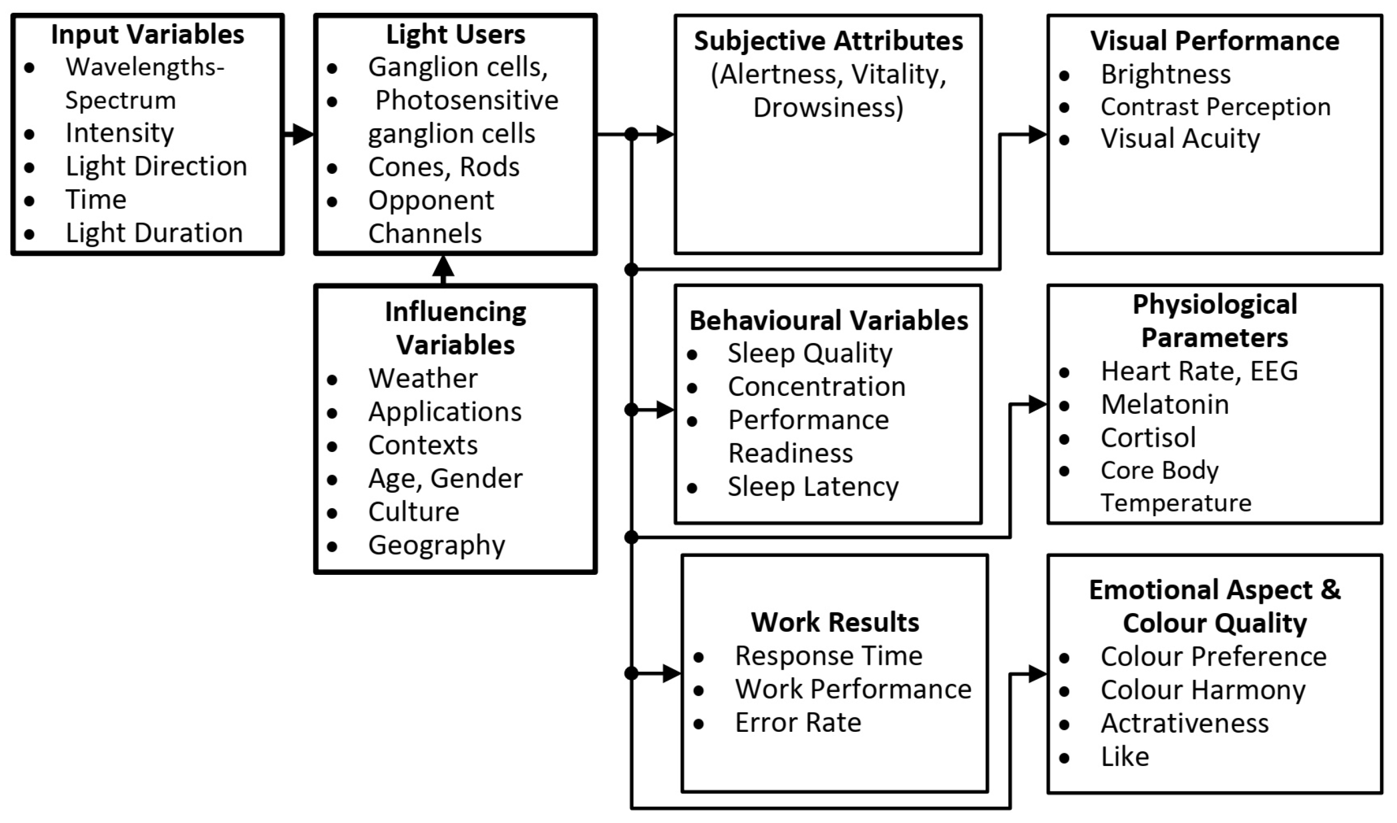
- Which input parameters can be used to describe the non-visual effects of light in their variety of manifestations (alertness, sleep quality, hormone production and suppression, and phase shift)?
- What values of these input variables are currently considered in the literature to be minimal, maximal, or optimal?
- Which measuring devices, sensor systems, and measuring methods can be used to measure the input quantities for non-visual lighting effects and process them in the context of smart lighting in the course of the control and regulation of LED or OLED luminaires on the basis of the definition of personal and room-specific applications?
- (a)
- “Daytime light recommendations for indoor environments: Throughout the daytime, the recommended minimum melanopic EDI is 250 lux at the eye measured in the vertical plane at approximately 1.2 m height (i.e., the vertical illuminance at eye level when seated)”.
- (b)
- “Evening light recommendations for residential and other indoor environments: During the evening, starting at least 3 h before bedtime, the recommended maximum melanopic EDI is 10 lux measured at the eye in the vertical plane approximately 1.2 m height. To help achieve this, where possible, white light should have a spectrum depleted in short wavelengths close to the peak of the melanopic action spectrum”.
- (c)
- “Nighttime light recommendations for the sleep environment: The sleep environment should be as dark as possible. The recommended maximum ambient melanopic EDI is 1 lux measured at the eye”.
- The determination and measurement of non-visual parameters after the completion of new lighting installations and comparison with the specifications of the previous lighting design; or verification of the results of the development of new luminaires for HCL lighting in the lighting laboratory or in the field. For this purpose, absolute spectroradiometers for spectral radiance or spectral irradiance are used to calculate the parameters and at different locations in the building. These two non-visual parameters cannot be measured directly with integral colorimeters and illuminance–luminance meters.
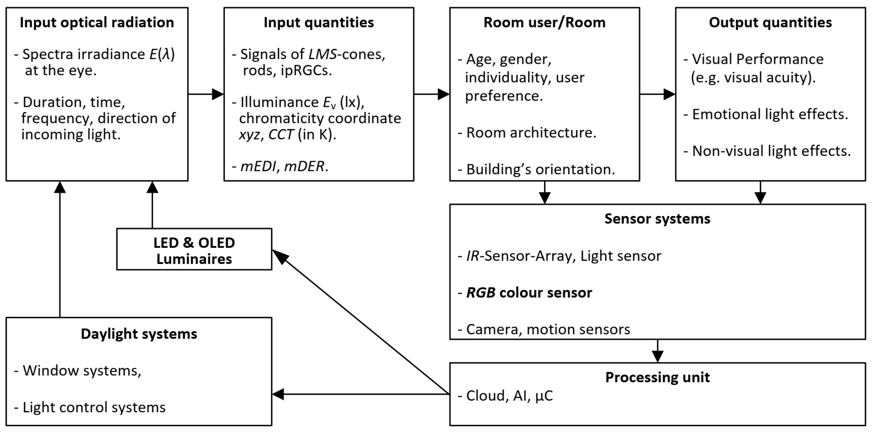
- The control or regulation of modern semiconductor-based lights (LED-OLED) and window systems (daylight systems) with the help of sensors in the room (e.g., presence sensors, position sensors, light and color sensors) [33]. In order to achieve a predefined value of non-visual parameters such as at a specific location in the room (e.g., in the center of the room or at locations further away from the windows), while taking into account dynamically changing weather conditions and the whereabouts of the room users, in practice, relatively inexpensive but sufficiently accurate optical sensors ( sensors) are required. The goal is to obtain not only the target photometric and colorimetric parameters such as illuminance (in lx), chromaticity coordinates (x, y, z), or correlated color temperature ( in K), but also the non-visual parameters and . The principle of this Smart Lighting concept using color sensors is illustrated in Figure 2. The methods for measuring non-visual parameters with low-cost but well-qualified color sensors are the content of the Section 3 and Section 4 and the focus of this paper.
2. Definition of Non-Visual Input Parameters [28]
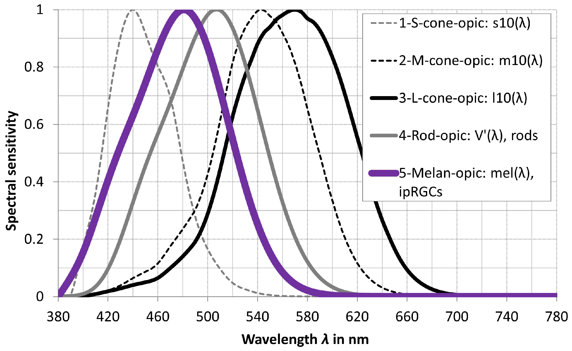
- S-cone-opic, ;
- M-cone-opic, ;
- L-cone-opic, ;
- Rhodopic, , rods;
- Melanopic, , ipRGCs.
- is the illuminance of the standard daylight illuminant D65 that has as much melanopic efficacy as the test light source for a given illuminance (lx) caused by the test light source. See Equation (6) in Table 3.
- is the ratio of the illuminance of the standard illuminant D65 () to the illuminance of the test illuminant (in lx) when the absolute melanopic efficacy of both illuminants is set equal. See Equation (9) in Table 3.
3. RGB Color Sensors: Characterization and Signal Transformation
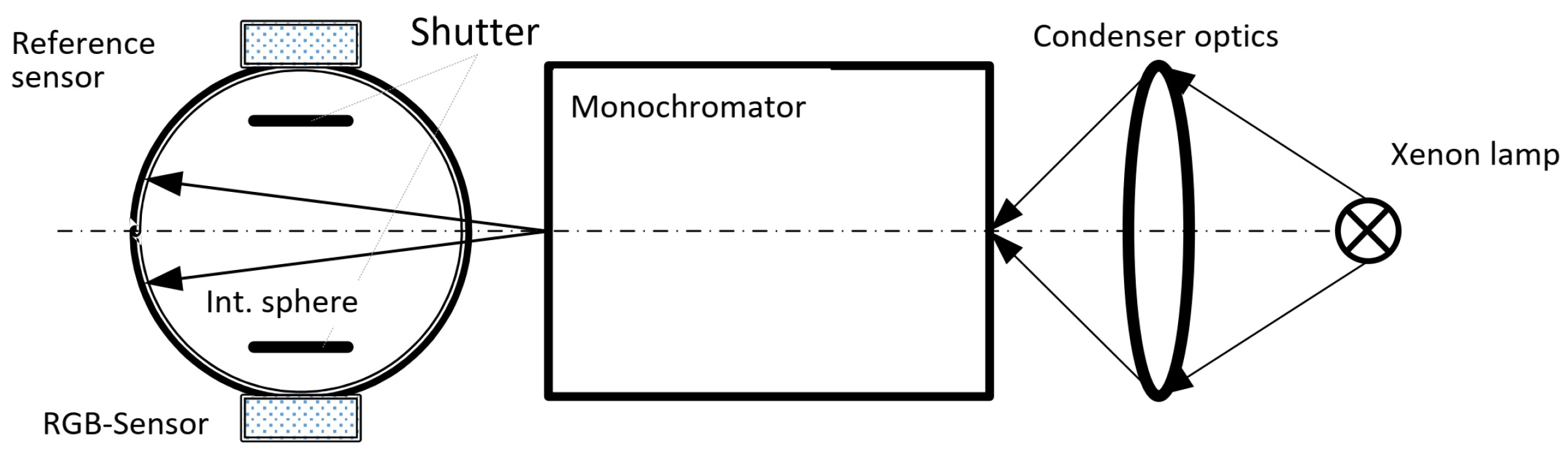
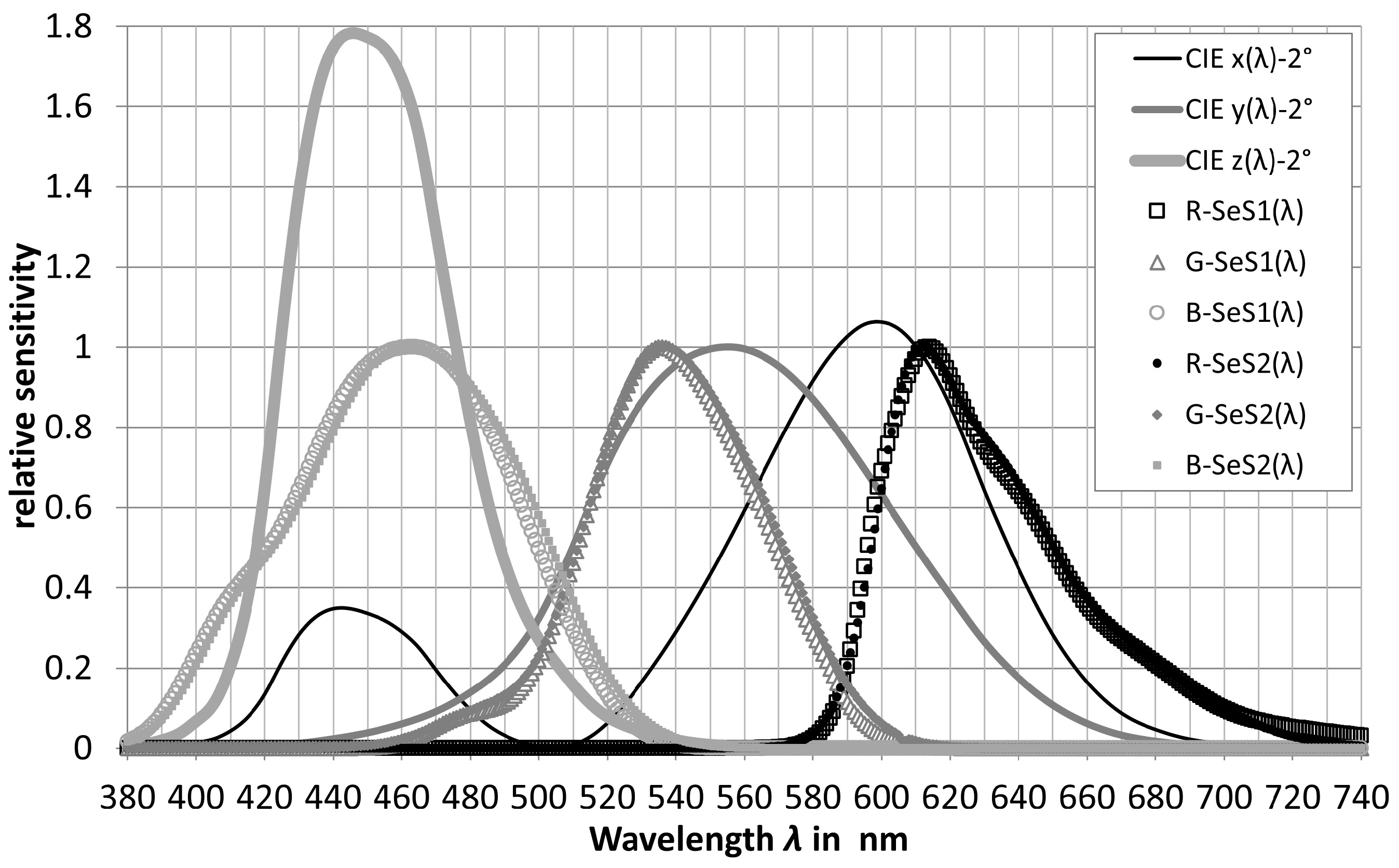
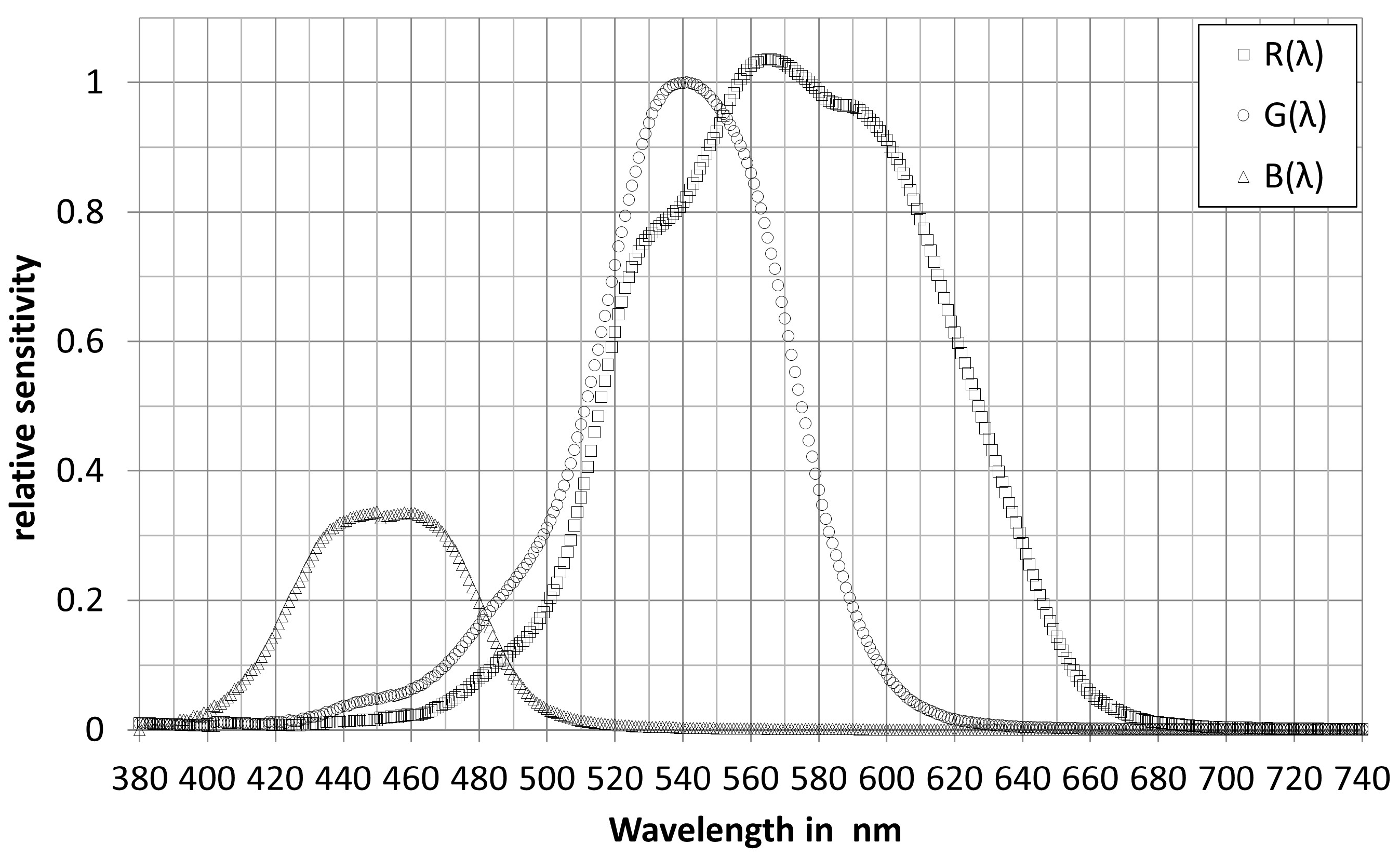
3.1. Characterisation of Color Sensors
- is the spectral sensitivity of the silicon sensor;
- is the spectral transmittance of the cos diffusor;
- is the spectral transmittance of the color filter layer for the respective color channel i = R, G, B;
- , , and are absolute factors to account for current-to-voltage conversion and voltage digitization;
- values are output signals (analog or digital) of the respective R–G–B color sensor at wavelength .
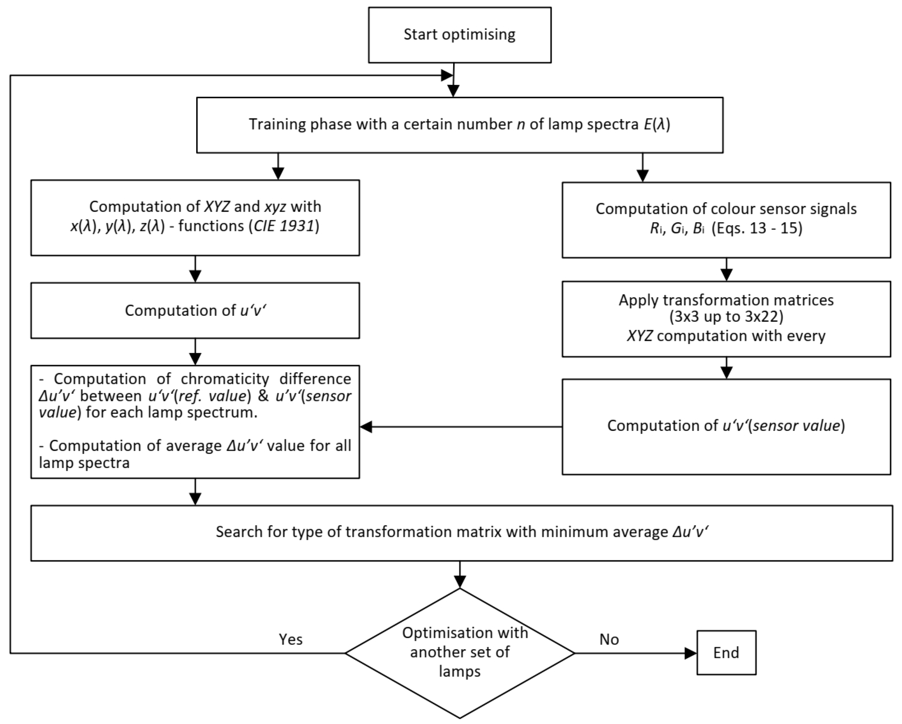
3.2. Method of Signal Transformation from to
3.3. Matrix Transformation in Practice and Verification with a Real Color Sensor
- (a)
- The deviation of the illuminances, calculated directly from the lamp spectra via the color sensor signals and via the formula in Table 7, was below 0.65% in percentage terms;
- (b)
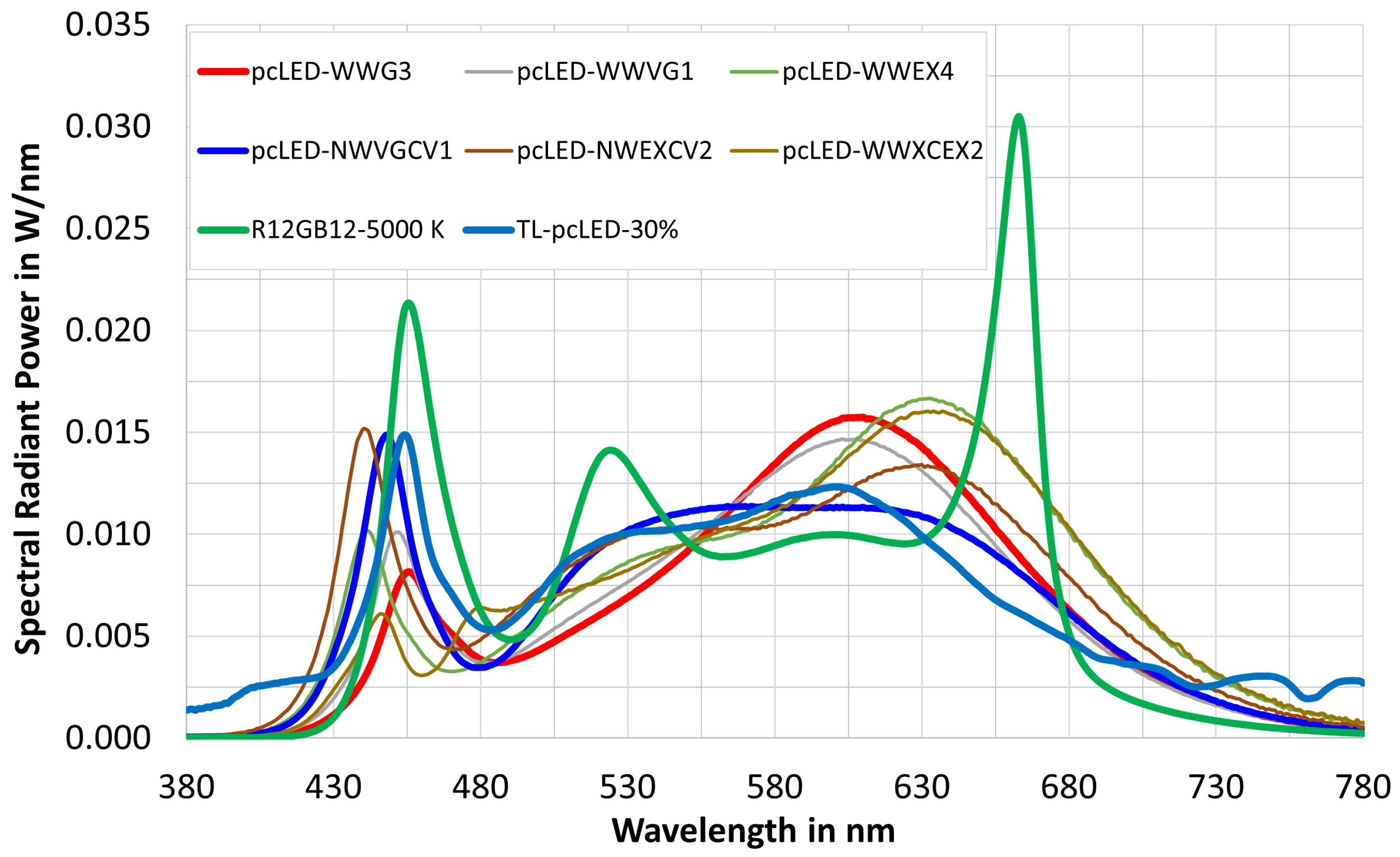
- For the majority of pc-LEDs and for the combinations daylight–white s, the chromaticity difference was in a small or moderately small range from the point of view of practical lighting technology, although the matrix transformation was synthesized only for the general case of many lamp types. No specific procedure was optimized for the specific case of only mixed light between daylight and conventional light, but the color and illuminance difference was still very small when using the achieved matrix transformation. Therefore, the authors did not build a separate case of mixed light with specific matrix transformation. Also, pc-LEDs and their mixing with daylight are dominant nowadays, so this verification in this way makes sense for applications. Therefore, the extreme cases of very complicated spectral shapes are not necessary to investigate their feasibility, because they are very rarely applied in today’s life. And an exception is the spectrum R12GB12-5000 K (green curve in Figure 10) with three distinct peaks of the three s (B around 455 nm, G around 525 nm, R around 660 nm), which is a very good demonstration example of a complicated spectral form. In this case, the color difference was .
4. Prediction of a Simple Computational Model for the Non-Visual Quantity and Verification of the Feasibility of a Sensor Using this Model
5. Conclusions and Discussion
Author Contributions
Funding
Institutional Review Board Statement
Informed Consent Statement
Data Availability Statement
Conflicts of Interest
References
- Rea, M.S.; Ouellette, M.J. Relative Visual Performance: A Basis for Application; SAGE Publications Sage UK: London, UK, 1991; Volume 23, pp. 135–144. [Google Scholar] [CrossRef]
- Rea, M.S.; Ouellette, M.J. Visual performance using reaction times. Light. Res. Technol. 1988, 20, 139–153. [Google Scholar] [CrossRef]
- Weston, H.C. The Relation between Illumination and Visual Efficiency-The Effect of Brightness Contrast. In The Relation between Illumination and Visual Efficiency-The Effect of Brightness Contrast; H.M. Stationery Office: London, UK, 1945. [Google Scholar]
- Boyce, P.R. Human Factors in Lighting; CRC Press: Boca Raton, FL, USA, 2014. [Google Scholar] [CrossRef]
- Lindner, H. Beleuchtungsstärke und Arbeitsleistung–Systematik experimenteller Grundlagen (Illumination levels and work performance–systematic experimental principles). Zeitschrift für Die Gesamte Hygiene und Ihre Grenzgebiete (J. Hyg. Relat. Discip.) 1975, 22, 101–107. [Google Scholar]
- Schmidt-Clausen, H.J.; Finsterer, H. Beleuchtung eines Arbeitsplatzes mit erhöhten Anforderungen im Bereich der Elektronik und Feinmechanik, 2nd ed.; Fachverlag NW in Carl Ed. Schünemann KG, 1989; ISBN-10: 388314925X, ISBN-13: 978-3883149257. [Google Scholar]
- Blackwell, H.R. Contrast thresholds of the human eye. J. Opt. Soc. Am. 1946, 36, 624–643. [Google Scholar] [CrossRef] [PubMed]
- Commission International de l’Eclairage (CIE). An Analytical Model for Describing the Influence of Lighting Parameters upon Visual Performance. 1981. Available online: https://cie.co.at/publications/analytic-model-describing-influence-lighting-parameters-upon-visual-performance-2nd-0 (accessed on 21 April 2023).
- DIN Deutsches Institut für Normung. DIN EN 12464-1 Light and Lighting—Lighting of Work Places—Part 1: Indoor Work Places. (2019). Available online: https://www.din.de/en/getting-involved/standards-committees/fnl/drafts/wdc-beuth:din21:302583817?destinationLanguage=&sourceLanguage (accessed on 21 April 2023).
- Houser, K.W.; Tiller, D.K.; Bernecker, C.A.; Mistrick, R. The subjective response to linear fluorescent direct/indirect lighting systems. Light. Res. Technol. 2002, 34, 243–260. [Google Scholar] [CrossRef]
- Tops, M.; Tenner, A.; Van Den Beld, G.; Begemann, S. The Effect of the Length of Continuous Presence on the Preferred Illuminance in Offices. In Proceedings CIBSE Lighting Conference; 1998; Available online: https://research.tue.nl/en/publications/the-effect-of-the-length-of-continuous-presence-on-the-preferred- (accessed on 21 April 2023).
- Juslén, H. Lighting, Productivity and Preferred Illuminances: Field Studies in the Industrial Environment; Helsinki University of Technology Helsinki: Espoo, Finland, 2007. [Google Scholar]
- Moosmann, C. Visueller Komfort und Tageslicht am Bueroarbeitsplatz: Eine Felduntersuchung in neun Gebaeuden; KIT Scientific Publishing: Karlsruhe, Deutschand, 2015. [Google Scholar]
- Park, B.C.; Chang, J.H.; Kim, Y.S.; Jeong, J.W.; Choi, A.S. A study on the subjective response for corrected colour temperature conditions in a specific space. Indoor Built Environ. 2010, 19, 623–637. [Google Scholar] [CrossRef]
- Lee, C.W.; Kim, J.H. Effect of LED lighting illuminance and correlated color temperature on working memory. Int. J. Opt. 2020, 2020, 3250364. [Google Scholar] [CrossRef]
- Fleischer, S.E. Die Psychologische Wirkung Veränderlicher Kunstlichtsituationen auf den Menschen. Ph.D. Thesis, ETH Zurich, Zürich, Switzerland, 2001. [Google Scholar]
- Bodrogi, P.; Brückner, S.; Krause, N.; Khanh, T.Q. Semantic interpretation of color differences and color-rendering indices. Color Res. Appl. 2014, 39, 252–262. [Google Scholar] [CrossRef]
- de Boer, J.B.D.F. Interior Lighting; Macmillan: London, UK, 1978. [Google Scholar]
- Balder, J. Erwunschte Leuchtdichten in Buroraumen (Preferred Luminace in Offices). Lichttechnik 1957, 9, 455–461. [Google Scholar]
- Khanh, T.Q.; Bodrogi, P.; Trinh, Q.V. Beleuchtung in Innenräumen–Human Centric Integrative Lighting Technologie, Wahrnehmung, Nichtvisuelle Effekte; Wiley-VCH: Berlin, Germany, 2022. [Google Scholar]
- Lok, R.; Smolders, K.C.; Beersma, D.G.; de Kort, Y.A. Light, alertness, and alerting effects of white light: A literature overview. J. Biol. Rhythm. 2018, 33, 589–601. [Google Scholar] [CrossRef] [PubMed]
- Souman, J.L.; Tinga, A.M.; Te Pas, S.F.; Van Ee, R.; Vlaskamp, B.N. Acute alerting effects of light: A systematic literature review. Behav. Brain Res. 2018, 337, 228–239. [Google Scholar] [CrossRef] [PubMed]
- Dautovich, N.D.; Schreiber, D.R.; Imel, J.L.; Tighe, C.A.; Shoji, K.D.; Cyrus, J.; Bryant, N.; Lisech, A.; O’Brien, C.; Dzierzewski, J.M. A systematic review of the amount and timing of light in association with objective and subjective sleep outcomes in community-dwelling adults. Sleep Health 2019, 5, 31–48. [Google Scholar] [CrossRef] [PubMed]
- Rea, M.S.; Figueiro, M. Light as a circadian stimulus for architectural lighting. Light. Res. Technol. 2018, 50, 497–510. [Google Scholar] [CrossRef]
- Rea, M.S.; Nagare, R.; Figueiro, M.G. Predictions of melatonin suppression during the early biological night and their implications for residential light exposures prior to sleeping. Sci. Rep. 2020, 10, 14114. [Google Scholar] [CrossRef] [PubMed]
- Rea, M.S.; Nagare, R.; Figueiro, M.G. Modeling circadian phototransduction: Quantitative predictions of psychophysical data. Front. Neurosci. 2021, 15, 615322. [Google Scholar] [CrossRef] [PubMed]
- Truong, W.; Trinh, V.; Khanh, T. Circadian stimulus–A computation model with photometric and colorimetric quantities. Light. Res. Technol. 2020, 52, 751–762. [Google Scholar] [CrossRef]
- Commission International de l’Eclairage (CIE). CIE S 026/E: 2018: CIE System for Metrology of Optical Radiation for ipRGC-Influenced Responses to Light; CIE Central Bureau: Vienna, Austria, 2018. [Google Scholar] [CrossRef]
- Commission International de l’Eclairage (CIE). CIE S 026. 2020: User Guide to the α-Opic Toolbox for Implementing; CIE Central Bureau: Vienna, Austria, 2020. [Google Scholar] [CrossRef]
- Houser, K.W.; Esposito, T. Human-centric lighting: Foundational considerations and a five-step design process. Front. Neurol. 2021, 12, 630553. [Google Scholar] [CrossRef] [PubMed]
- International WELL Building Institute pbc. The WELL Building Standard, Version 2. New York, NY, USA, 2020. Available online: https://v2.wellcertified.com/wellv2/en/overview (accessed on 25 April 2023).
- Brown, T.M.; Brainard, G.C.; Cajochen, C.; Czeisler, C.A.; Hanifin, J.P.; Lockley, S.W.; Lucas, R.J.; Münch, M.; O’Hagan, J.B.; Peirson, S.N.; et al. Recommendations for daytime, evening, and nighttime indoor light exposure to best support physiology, sleep, and wakefulness in healthy adults. PLoS Biol. 2022, 20, e3001571. [Google Scholar] [CrossRef] [PubMed]
- Fan, B.; Zhao, X.; Zhang, J.; Sun, Y.; Yang, H.; Guo, L.J.; Zhou, S. Monolithically Integrating III-Nitride Quantum Structure for Full-Spectrum White LED via Bandgap Engineering Heteroepitaxial Growth. Laser Photonics Rev. 2023, 17, 2200455. [Google Scholar] [CrossRef]
- ISO/CIE TR 21783:2022|ISO/CIE TR 21783; Light and Lighting—Integrative Lighting—Non-Visual Effects. ISO: Geneva, Switzerland, 2022.
- Commission Internationale de l’Éclairage (CIE). Colourimetry, 2018. Available online: https://onlinelibrary.wiley.com/doi/10.1002/col.22387 (accessed on 4 April 2023).
- Westland, S.; Ripamonti, C.; Cheung, V. Computational Colour Science Using MATLAB; John Wiley & Sons: Hoboken, NJ, USA, 2012. [Google Scholar]
- Bieske, K. Über die Wahrnehmung von Lichtfarbenänderungen zur Entwicklung Dynamischer Beleuchtungssysteme. Ph.D. Thesis, Technische Universität Ilmenau, 2010. Available online: https://d-nb.info/1002583519/04 (accessed on 25 April 2023).


| No. | Parameter | Preferred Values |
|---|---|---|
| 1 | Horizontal illuminance in lux [11,12,13] | Greater than 850 lx; Recommended range: 1300 lx–1500 lx |
| 2 | Correlated color temperature in K [14,15] | 4000 K–5000 K |
| 3 | Color rendering index [17] | >87 |
| 4 | Indirect to total illuminance ratio [10,16] | >0.6–0.8 |
| -Opic Quantities | ||
|---|---|---|
| Parameter | Equation | Equation No. |
| -opic-radian flux | similar to (3.1) Page 4 [28] | |
| -opic-radiance | similar to (3.5) Page 4 [28] | |
| -opic-irradiance | similar to (3.6) Page 5 [28] | |
| -Opic Quantities | ||
|---|---|---|
| Parameter | Equation | Equation No. |
| Melanopic Equivalent Daylight (D65) Illuminance (mEDI) in lx | similar to (3.9) Page 6 [28] with =mel. | |
| ↓ | ||
| Melanopic Daylight (D65) Efficacy Ratio () | ↓ | |
| similar to (3.10) Page 7 [28] with =mel. | ||
| (*) Note: For the parameter (indices x, y according to the corresponding definitions), see Equations (4) and (5) when = mel, and apply Equation (3) when the calculated parameter is the mel-opic irradiance. | ||
| Nr. | Size | Content |
|---|---|---|
| 1 | 3 × 3 | [R G B] |
| 2 | 3 × 5 | [R G B 1] |
| 3 | 3 × 7 | [R G B RG RB GB 1] |
| 4 | 3 × 8 | [R G B RG RB GB 1] |
| 5 | 3 × 10 | [R G B RG RB GB 1] |
| 6 | 3 × 11 | [R G B RG RB GB 1] |
| 8 | 3 × 14 | [R G B RG RB GB 1] |
| 9 | 3 × 16 | [R G B RG RB GB G B R ] |
| 10 | 3 × 17 | [R G B RG RB GB G B R 1] |
| 11 | 3 × 19 | [R G B RG RB GB G B R B R G ] |
| 12 | 3 × 20 | [R G B RG RB GB G B R B R G 1] |
| 13 | 3 × 22 | [R G B RG RB GB G B R B R G GB RB RG] |
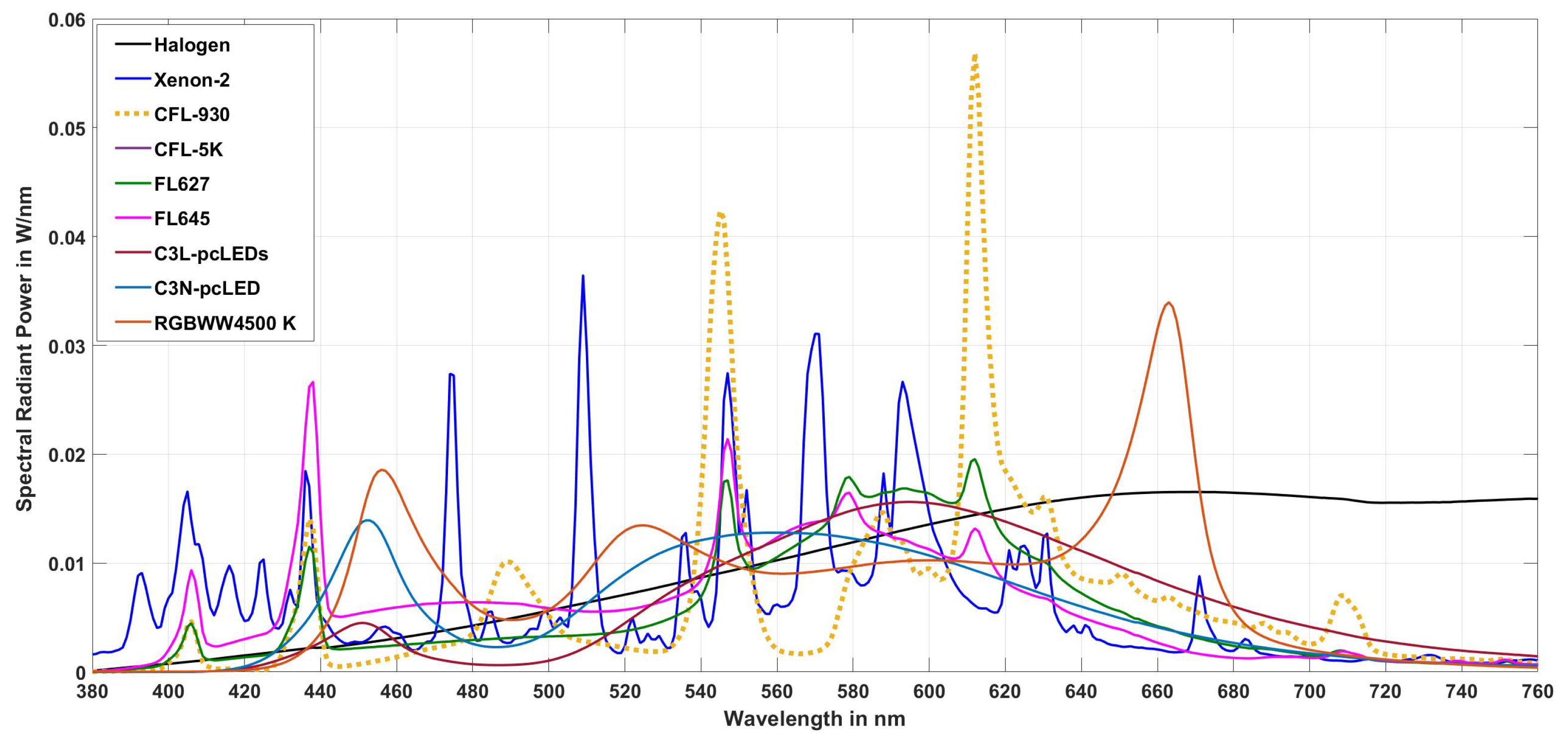
| Lamp Type | Tungsten Halogen | Xenon-2 | CFL 3000 K | CFL 5000 K | FL 627 | FL 645 | LED C3L | LED c3N | LED RGBWW4500 |
|---|---|---|---|---|---|---|---|---|---|
| (in K) | 2762 | 4100 | 2640 | 4423 | 2785 | 4423 | 2640 | 4580 | 4500 |
| () | 3 | 7.2 | 0.61 | 2.2 | 1.8 | 2.2 | 6.3 | 1.3 | −1.0 |
| CIE | 85 | −86 | 48 | −60 | −72 | −60 | −28 | −39 | 36 |
| CIE | 97 | 67 | 90 | 68 | 64 | 68 | 67 | 69 | 90 |
| Name | Xenon-2 | CFL-930 | CFL-5K | FL627 | FL645 | C3L-pcLEDs | C3N-pcLED | RGBWW4500 K | Max |
|---|---|---|---|---|---|---|---|---|---|
| 7.4 | 7.7 | 1.5 | 4.5 | 1.5 | 0.42 | 2.7 | 8.3 | 8.3 | |
| 4.8 | 48 | 12 | 41 | 12 | 51 | 16 | 16 | 51 | |
| 8.5 | 5.3 | 1.6 | 7.0 | 20 | 6.4 | 20 | |||
| 6.9 | 32 | 11 | 40 | 11 | 48 | 7.0 | 16 | 48 | |
| 2.9 | 4.5 | 0.92 | 12 | 3.8 | 12 | ||||
| 7.9 | 2.2 | 37 | 2.2 | 42 | 12 | 8.1 | 42 | ||
| 7.1 | 10 | 7.8 | 1.7 | 6.7 | 10 | ||||
| 8.4 | 5.7 | 3.0 | 2.5 | 1.9 | 10 | 10 | |||
| 8.4 | 5.7 | 3.0 | 2.5 | 1.9 | 10 | 10 | |||
| 7.2 | 9.1 | 4.3 | 5.7 | 7.5 | 9.1 | ||||
| 7.2 | 9.1 | 4.3 | 5.7 | 7.5 | 9.1 | ||||
| 6.6 | 8.9 | 2.2 | 3.2 | 7.2 | 8.9 |
| (lx) from R, G, B | |
| ; | |
| Matrix 3 × 3 in case of the 9 light sources of training set |
| Name | pcLED-WWG3 | pcLED-WWVG1 | vpcLED- WWEX4 | pcLED-NWVG1 | pcLED-NWEXCV2 | pcLED-CWEX2 | R12GB12-5000 K | TL-pcLED-30% |
|---|---|---|---|---|---|---|---|---|
| (K) | 2801 | 3105 | 2969 | 4614 | 3942 | 5059 | 5001 | 4391 |
| CRI | 84.06 | 85.63 | 94.41 | 90.91 | 93.09 | 95.99 | 89.73 | 89.85 |
| x | 0.4434 | 0.4217 | 0.4252 | 0.3569 | 0.3764 | 0.3439 | 0.3449 | 0.3644 |
| y | 0.3929 | 0.3841 | 0.3765 | 0.3608 | 0.3550 | 0.3557 | 0.3495 | 0.3650 |
| 752.29 | 752.54 | 754.17 | 751.40 | 754.79 | 750.01 | 747.60 | 751.94 | |
| 0.4434 | 0.4217 | 0.4252 | 0.3546 | 0.3779 | 0.3368 | 0.3319 | 0.3665 | |
| 0.3929 | 0.3841 | 0.3765 | 0.3643 | 0.3698 | 0.3571 | 0.3529 | 0.3696 | |
| 1.36 | 1.20 | 1.68 | 3.15 | 8.76 | 5.32 | 10.1 | 2.42 | |
| in % | 0.31 | 0.34 | 0.56 | 0.19 | 0.64 | 0.00 | -0.32 | 0.26 |
| (lx) from R, G, B | |
| ; | |
| Matrix 3 × 3 in the case of the 9 light sources of the training set |
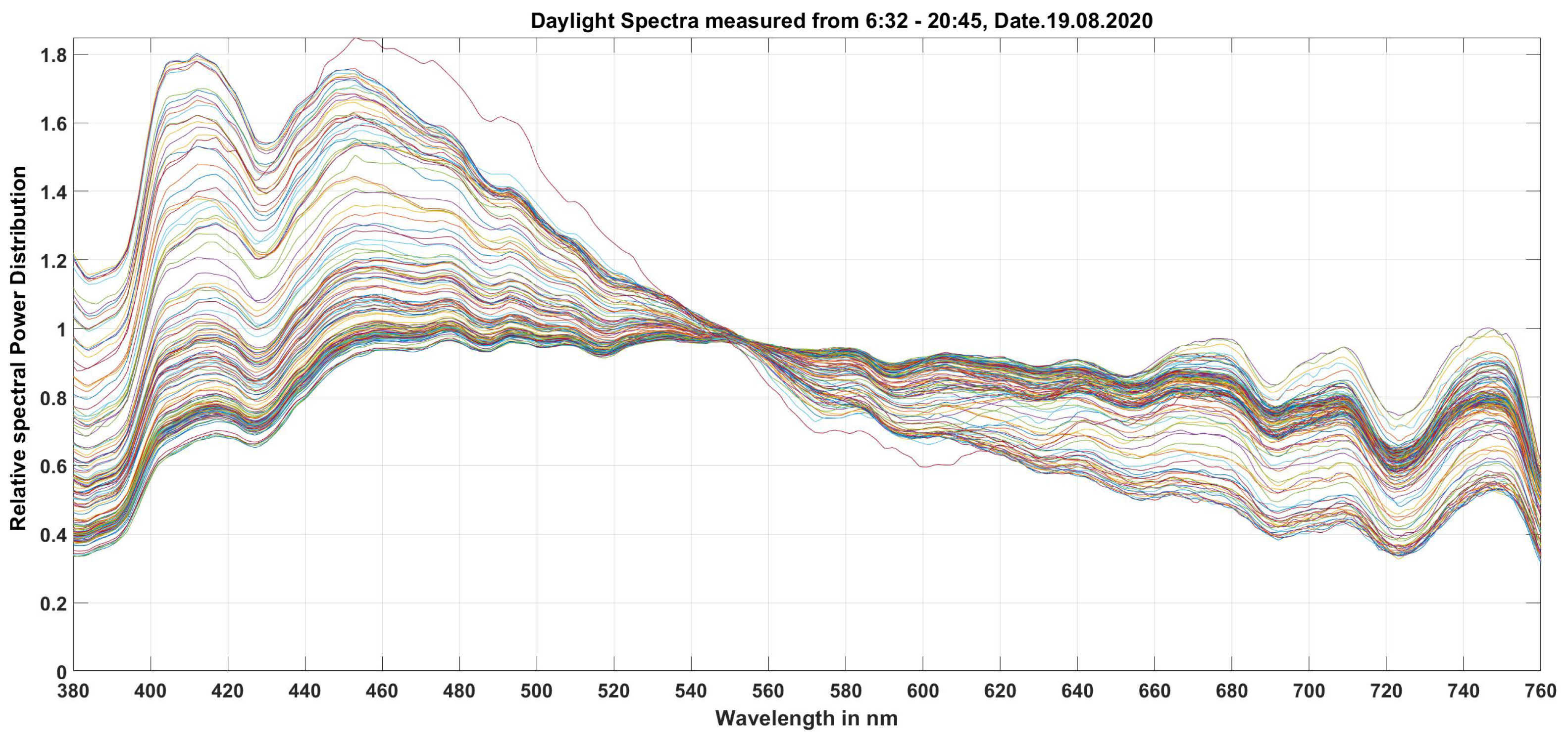
| Sampling Time | 07:27:17 | 10:03:31 | 11:06:01 | 12:03:19 | 13:05:50 | 14:07:40 | 15:10:10 | 16:12:41 | 19:14:58 |
|---|---|---|---|---|---|---|---|---|---|
| in K | 12,464 | 8033 | 6313 | 5651 | 5914 | 5853 | 5470 | 8174 | 16,066 |
| in lx | 401 | 9397 | 23,940 | 58,212 | 39,463 | 43,150 | 71,006 | 15,058 | 461 |
| 0.2831 | 0.3066 | 0.3293 | 0.3413 | 0.3364 | 0.3376 | 0.3449 | 0.3081 | 0.2705 | |
| in lx | 400.60 | 9403.02 | 23,944.07 | 58,205.57 | 39,465.20 | 43,149.59 | 70,987.13 | 15,070.62 4 | 60.41 |
| 4.75 | 1.74 | 1.20 | 1.82 | 1.96 | 0.596 | 4.03 | 8.57 |
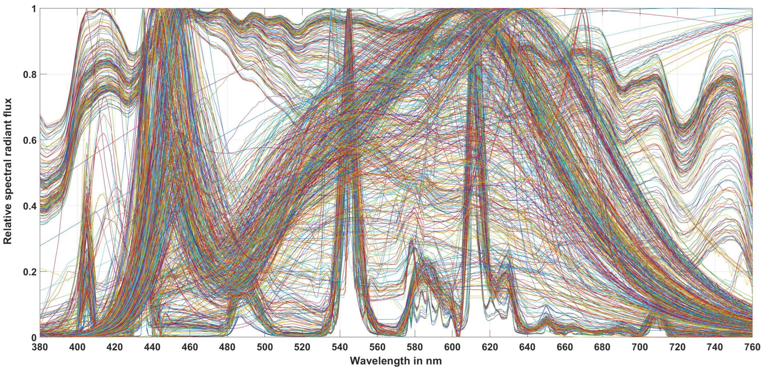
| No. | Type of light sources and their parameter ranges = 2201 – 17,815 K; −1.467× < < 1.529× 0.0797 < z < 0.4792; 80 < < 100; 0.2784 < < 1.46 |
| 1. | Conventional incandescent lamps + filtered incandescent lamps |
| 2. | Fluorescent tubes + Compact fluorescent lamps |
| 3. | LED lamps + LED luminaires |
| 4. | Daylight (CIE-model + measurements) |
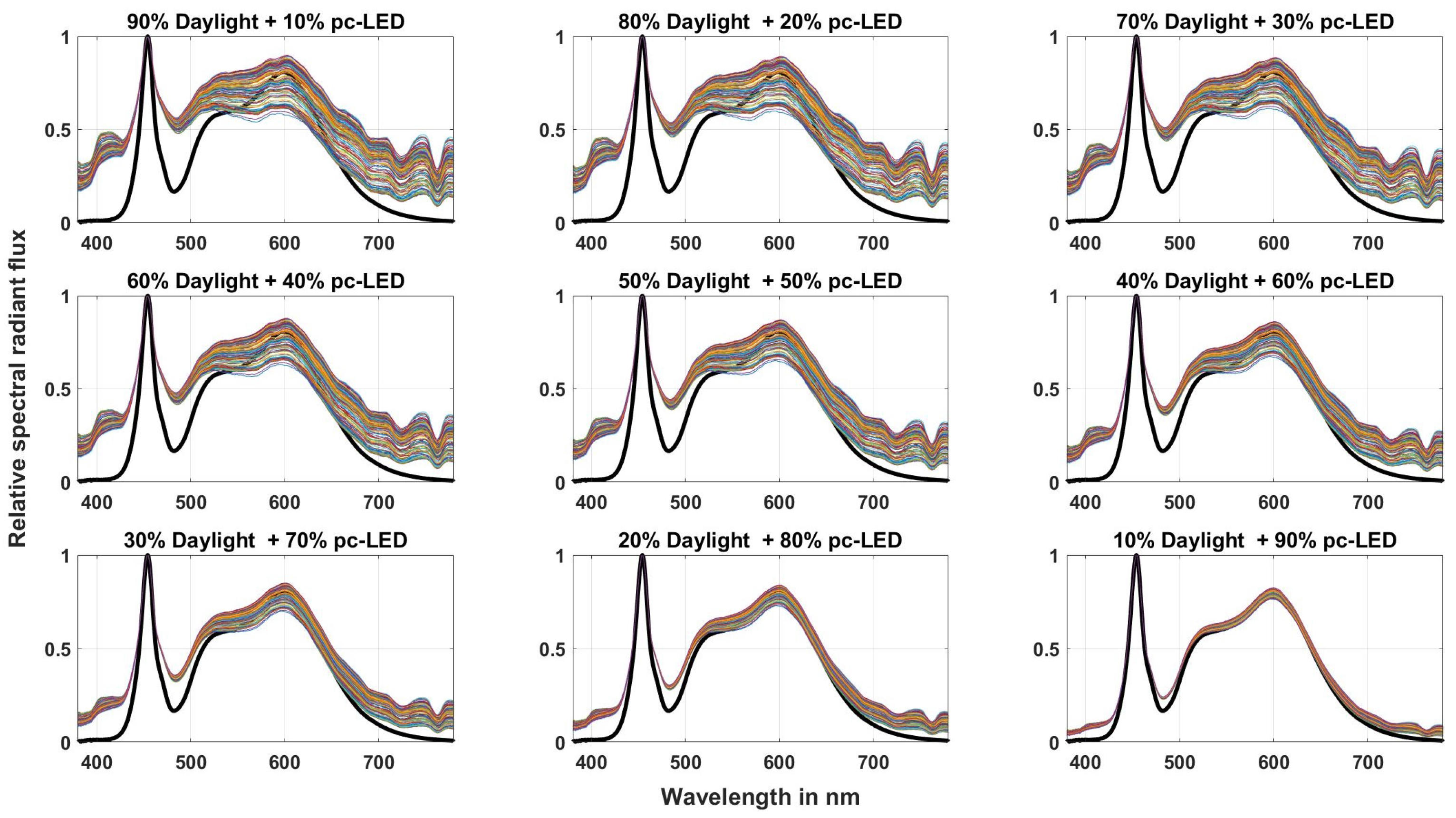
| 5. | Mixtures (DL+LED) − [ mixture ratio = 10–90% ] |
| 6. | Mixtures (DL+FL) − [ mixture ratio = 10–90% ] |
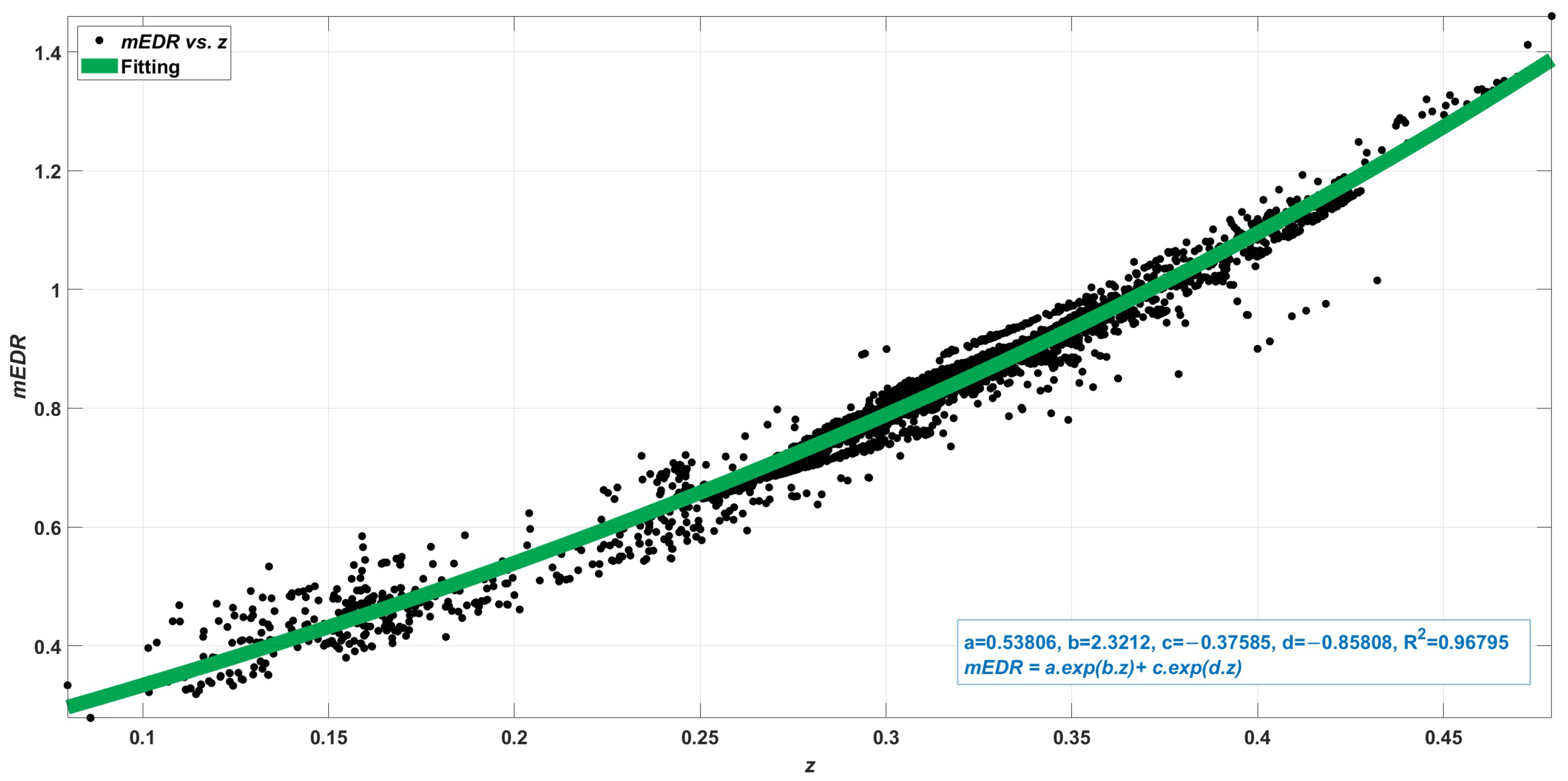
| Parameter | a | b | c | d | |
|---|---|---|---|---|---|
| Value | 0.53806 | 2.3212 | −0.37585 | −0.85808 | 0.968 |
| Name | pcLED-WWG3 | pcLED-WWVG1 | pcLED-WWEX4 | pcLED-NWVG1 | pcLED-NWEXCV2 | pcLED-CWEX2 | R12GB12-5000 K | TL-pcLED-30% |
|---|---|---|---|---|---|---|---|---|
| (K) | 2801 | 3105 | 2969 | 4614 | 3942 | 5059 | 5001 | 4391 |
| CIE | 84.06 | 85.63 | 94.41 | 90.91 | 93.09 | 95.99 | 89.73 | 89.85 |
| x | 0.4434 | 0.4217 | 0.4252 | 0.3569 | 0.3764 | 0.3439 | 0.3449 | 0.3644 |
| y | 0.3929 | 0.3841 | 0.3765 | 0.3608 | 0.3550 | 0.3557 | 0.3495 | 0.3650 |
| (lx) | 750 | 750 | 750 | 750 | 750 | 750 | 750 | 750 |
| 0.46 | 0.51 | 0.53 | 0.75 | 0.67 | 0.83 | 0.83 | 0.71 | |
| 347.67 | 383.55 | 395.93 | 562.91 | 500.06 | 625.10 | 625.79 | 532.40 | |
| (lx) | 752.29 | 752.54 | 754.17 | 751.40 | 754.79 | 750.01 | 747.60 | 751.94 |
| 0.4434 | 0.4217 | 0.4252 | 0.3546 | 0.3779 | 0.3368 | 0.3319 | 0.3665 | |
| 0.3929 | 0.3841 | 0.3765 | 0.3643 | 0.3698 | 0.3571 | 0.3529 | 0.3696 | |
| 0.46 | 0.53 | 0.54 | 0.74 | 0.66 | 0.81 | 0.83 | 0.69 | |
| 346.28 | 396.00 | 403.79 | 554.58 | 500.85 | 604.47 | 621.78 | 521.19 | |
| 1.36 × | 1.20 × | 1.68 × | 3.15 × | 8.76× | 5.32 × | 1.01 × | 2.42 × | |
| in % | 0.31 | 0.34 | 0.56 | 0.19 | 0.64 | 0.00 | −0.32 | 0.26 |
| in % | −0.7 | 2.9 | 1.4 | −1.7 | −0.5 | −3.3 | −0.3 | −2.4 |
| in % | 0.40 | 3.25 | 1.99 | 1.48 | 0.16 | 3.30 | 0.64 | 2.10 |
Disclaimer/Publisher’s Note: The statements, opinions and data contained in all publications are solely those of the individual author(s) and contributor(s) and not of MDPI and/or the editor(s). MDPI and/or the editor(s) disclaim responsibility for any injury to people or property resulting from any ideas, methods, instructions or products referred to in the content. |
© 2023 by the authors. Licensee MDPI, Basel, Switzerland. This article is an open access article distributed under the terms and conditions of the Creative Commons Attribution (CC BY) license (https://creativecommons.org/licenses/by/4.0/).
Share and Cite
Trinh, V.Q.; Bodrogi, P.; Khanh, T.Q. Determination and Measurement of Melanopic Equivalent Daylight (D65) Illuminance (mEDI) in the Context of Smart and Integrative Lighting. Sensors 2023, 23, 5000. https://doi.org/10.3390/s23115000
Trinh VQ, Bodrogi P, Khanh TQ. Determination and Measurement of Melanopic Equivalent Daylight (D65) Illuminance (mEDI) in the Context of Smart and Integrative Lighting. Sensors. 2023; 23(11):5000. https://doi.org/10.3390/s23115000
Chicago/Turabian StyleTrinh, Vinh Quang, Peter Bodrogi, and Tran Quoc Khanh. 2023. "Determination and Measurement of Melanopic Equivalent Daylight (D65) Illuminance (mEDI) in the Context of Smart and Integrative Lighting" Sensors 23, no. 11: 5000. https://doi.org/10.3390/s23115000
APA StyleTrinh, V. Q., Bodrogi, P., & Khanh, T. Q. (2023). Determination and Measurement of Melanopic Equivalent Daylight (D65) Illuminance (mEDI) in the Context of Smart and Integrative Lighting. Sensors, 23(11), 5000. https://doi.org/10.3390/s23115000