
Well Performance Classification and Prediction: Deep Learning and Machine Learning Long Term Regression Experiments on Oil, Gas, and Water Production

 ,
, 
Abstract
:1. Introduction
2. Related Works
2.1. Oil Flowrate Prediction
2.2. Well Production
2.3. Well Production Enhancement Prediction
- Multi-RNN: 5.523%
- Single GRU: 55.078%
- Multi-GRU/ANN: 72%
- Multi LSTM: 51%
- Stacked DGR: 70%
2.4. Pressure Gradient Prediction
2.5. Fault Prediction
- Based on the RNN-LSTM, SAE, and particle swarm optimization (PSO) approaches, a novel DL fault detection with a simple and effective framework is created to balance the three steps of parameter optimization, fault feature extraction, and fault detection.
- A novel hybrid mathematical approach can improve learning ability by addressing RNN training limitations such as decaying error, deficit, gradient vanishing, and backflow.
- The DL framework provides strong autonomous deep learning for unlabeled data, allowing the proposed DL approach to not only adapt the relevant features, but also to realize patterns without saving the prior sequence inputs.
- The suggested deep learning framework contributes to the field of electrical gas generator defect detection, which could be valuable for future industrial deep learning applications, particularly in dangerous environments.
2.6. Bottom-Hole Pressure Prediction
2.7. Reservoir Characterization
2.8. Related Work Summary
3. Methods and Materials
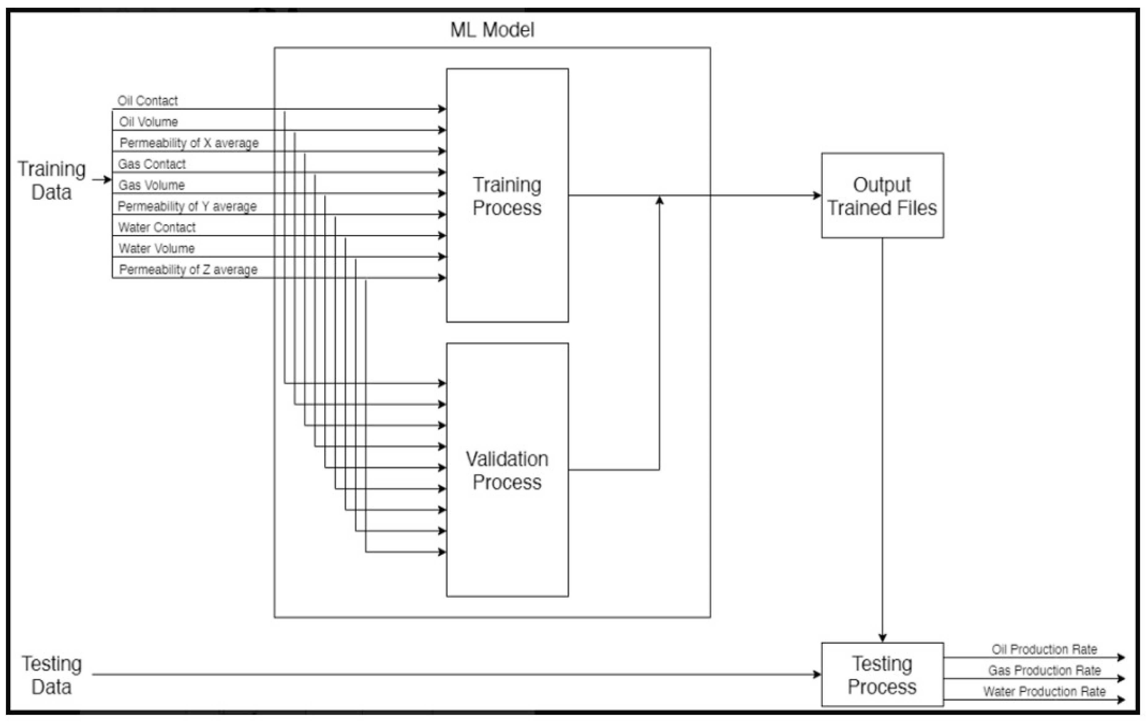
3.1. Dataset
3.2. Tools
3.3. Methods
3.3.1. MLR
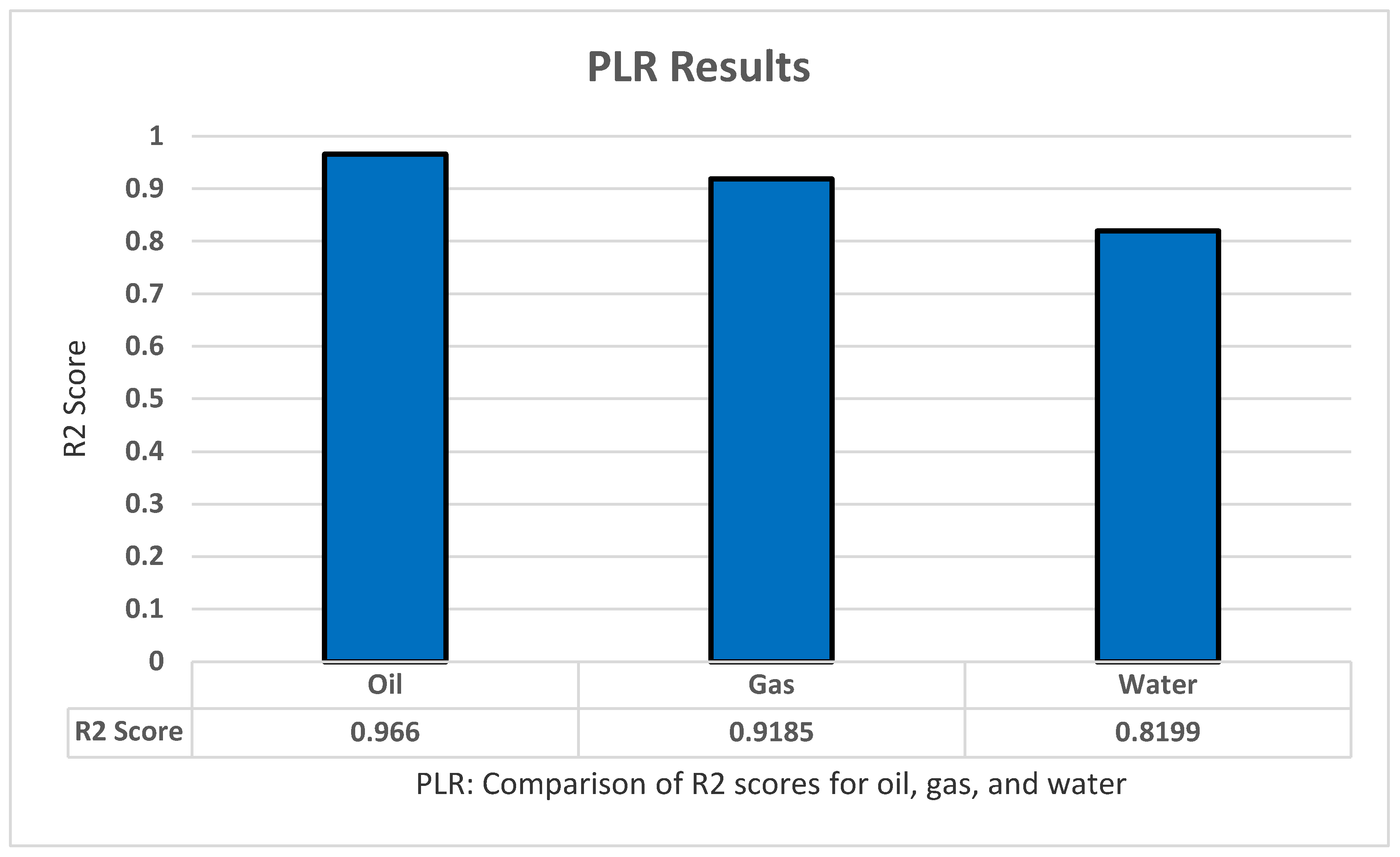
3.3.2. PLR
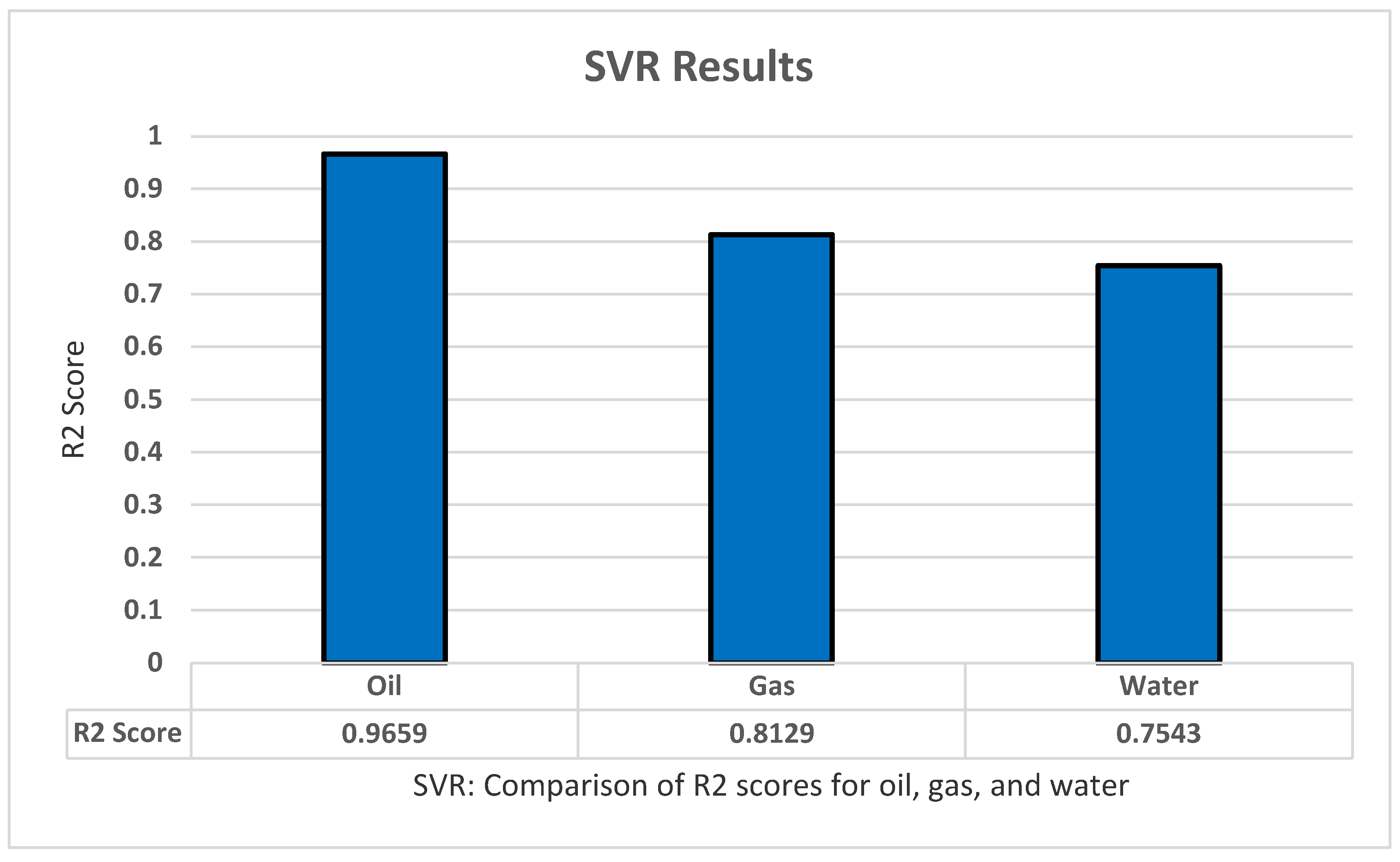
3.3.3. SVR
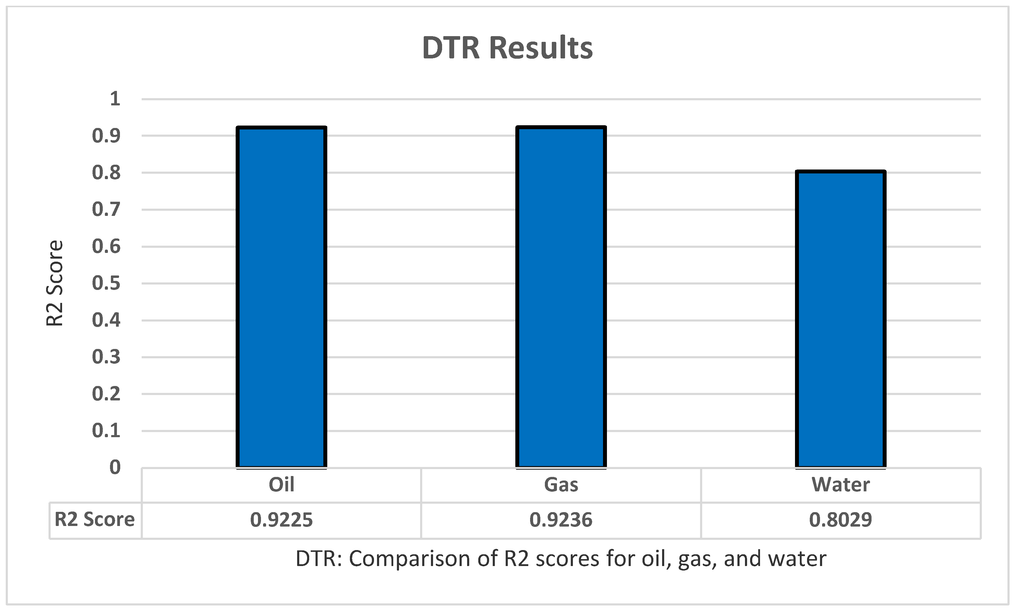
3.3.4. DTR
- Does performing the split increase the amount of information we have about our dataset?
- Does it add some value to the approach we would like to group our data points (information entropy)?
3.3.5. RFR
3.3.6. XGBoost

3.3.7. ANN
3.3.8. RNN
4. AI Model
5. Result and Analysis
5.1. MLR
5.2. PLR
5.3. SVR
5.4. DTR
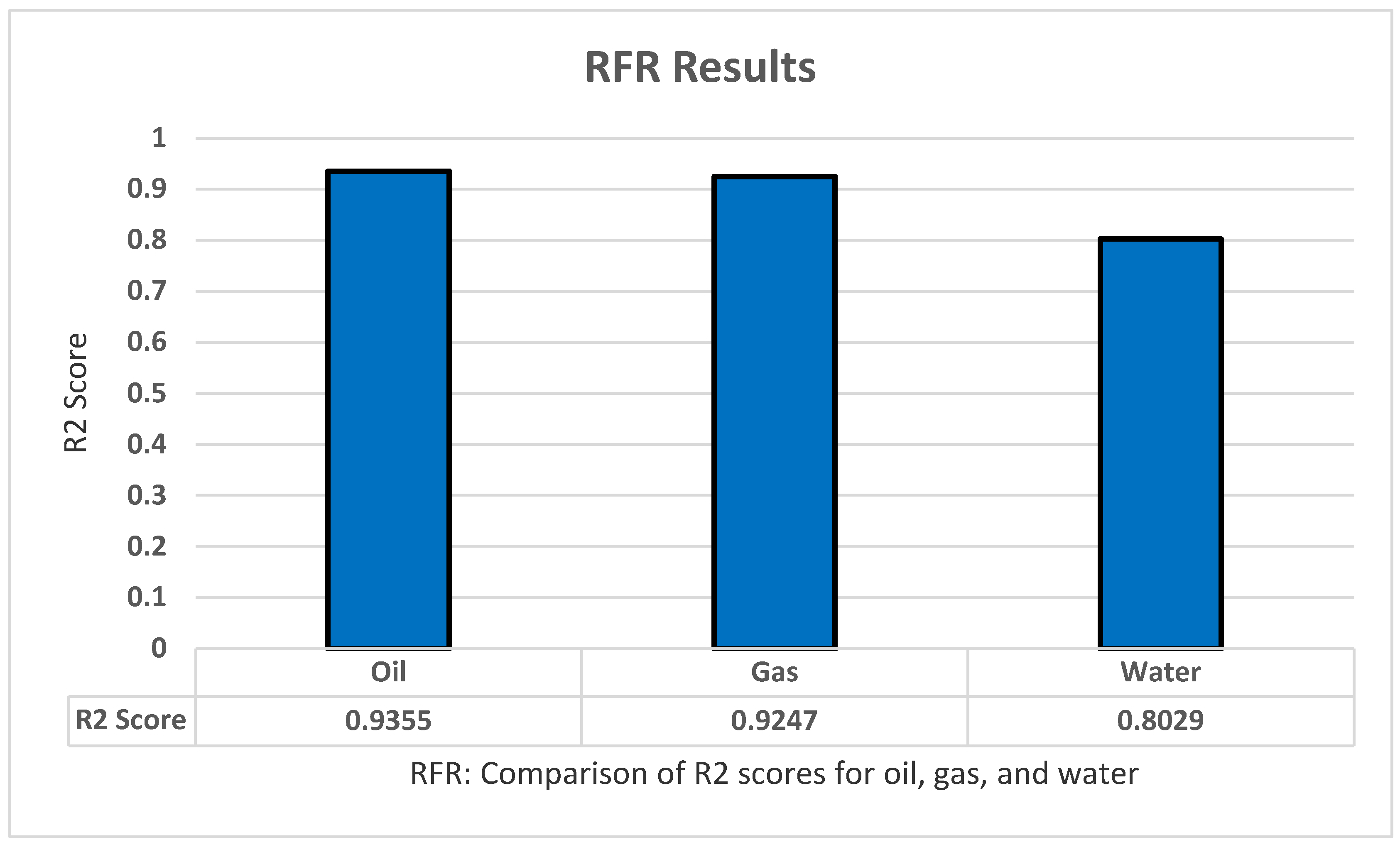
5.5. RFR
5.6. XGBoost
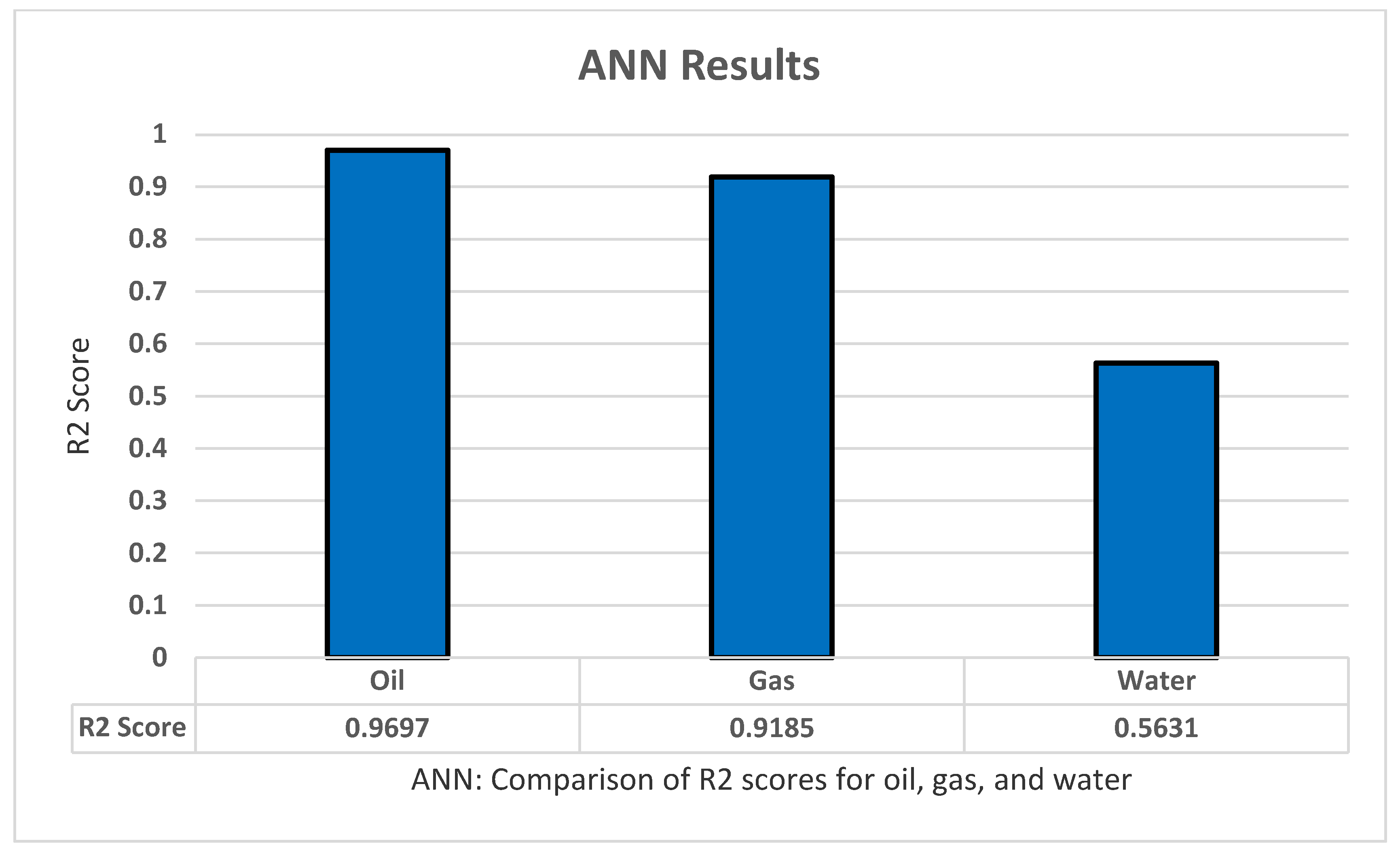
5.7. ANN
5.8. RNN(LSTM)
5.9. Experiments Discussion
6. Conclusions
- The results we achieved with ANN, XGBoost, and RNN are the highest, with a mean R2 for oil, gas, and water of 0.9627, 0.9012, and 0.926, respectively. We found that ML algorithms performed best with the default dataset while the other algorithms performed better in the custom dataset. Some methods had more significant results if the data were standardized before experimenting, such as SVR with a mean R2 of 0.9014. Other algorithms, however, performed better with a pure dataset such as RFR with a mean R2 of 0.8848. Normalizing the dataset for both the default and the custom datasets did not yield good results and was outperformed by pure and standardized data.
- After experimenting with the dataset and examining the results for every method selected, it is hard to say that these are the best results we can obtain. There is still plenty of room for improvement to achieve even better results by exploring different methods or a combination of methods. Nevertheless, the results we acquired are satisfactory considering the complexity of the problem.
7. Future Work
Author Contributions
Funding
Acknowledgments
Conflicts of Interest
References
- Abdullayeva, F.; Imamverdiyev, Y. Development of Oil Production Forecasting Method Based on Deep Learning. Optim. Inf. Comput. 2019, 7, 826–839. [Google Scholar] [CrossRef] [Green Version]
- al Ajmi, M.D.; Alarifi, S.A.; Mahsoon, A.H. Improving Multiphase Choke Performance Prediction and Well Production Test Validation Using Artificial Intelligence: A New Milestone. In Proceedings of the Society of Petroleum Engineers—SPE Digital Energy Conference and Exhibition 2015, The Woodlands, TX, USA, 3–5 March 2015. [Google Scholar] [CrossRef]
- Ghorbani, H.; Wood, D.A.; Choubineh, A.; Tatar, A.; Abarghoyi, P.G.; Madani, M.; Mohamadian, N. Prediction of Oil Flow Rate through an Orifice Flow Meter: Artificial Intelligence Alternatives Compared. Petroleum 2020, 6, 404–414. [Google Scholar] [CrossRef]
- Amaechi, U.C.; Ikpeka, P.M.; Xianlin, M.; Ugwu, J.O. Application of Machine Learning Models in Predicting Initial Gas Production Rate from Tight Gas Reservoirs. Rud.-Geol.-Naft. Zb. 2019, 34, 29–40. [Google Scholar] [CrossRef] [Green Version]
- Mirzaei-Paiaman, A.; Salavati, S. The Application of Artificial Neural Networks for the Prediction of Oil Production Flow Rate. Energy Sources 2012, 34, 1834–1843. [Google Scholar] [CrossRef]
- Han, D.; Kwon, S. Application of Machine Learning Method of Data-driven Deep Learning Model to Predict Well Production Rate in the Shale Gas Reservoirs. Energies 2021, 14, 3629. [Google Scholar] [CrossRef]
- Pal, M. On Application of Machine Learning Method for History Matching and Forecasting of Times Series Data from Hydrocarbon Recovery Process Using Water Flooding. Pet. Sci. Technol. 2021, 39, 519–549. [Google Scholar] [CrossRef]
- Doan, T.T.; van Vo, M. Using Machine Learning Techniques for Enhancing Production Forecast in North Malay Basin. In Springer Series in Geomechanics and Geoengineering; Springer: Singapore, 2020; pp. 114–121. [Google Scholar] [CrossRef]
- Negash, B.M.; Yaw, A.D. Artificial Neural Network Based Production Forecasting for a Hydrocarbon Reservoir under Water Injection. Pet. Explor. Dev. 2020, 47, 383–392. [Google Scholar] [CrossRef]
- Guo, Z.; Wang, H.; Kong, X.; Shen, L.; Jia, Y. Machine Learning-Based Production Prediction Model and Its Application in Duvernay Formation. Energies 2021, 14, 5509. [Google Scholar] [CrossRef]
- Jabbari, M.; Khushaba, R.; Nazarpour, K.; Han, S.; Zhong, X.; Shao, H.; Pan, S.; Wang, J.; Zhou, W. Prediction on Production of Oil Well with Attention-CNN-LSTM. J. Phys. Conf. Ser. 2021, 2030, 012038. [Google Scholar] [CrossRef]
- Xia, L.; Shun, X.; Jiewen, W.; Lan, M. Predicting Oil Production in Single Well Using Recurrent Neural Network. In Proceedings of the 2020 International Conference on Big Data, Artificial Intelligence and Internet of Things Engineering, ICBAIE, Fuzhou, China, 12–14 June 2020; pp. 423–430. [Google Scholar] [CrossRef]
- Nguyen-Le, V.; Shin, H. Artificial Neural Network Prediction Models for Montney Shale Gas Production Profile Based on Reservoir and Fracture Network Parameters. Energy 2022, 244, 123150. [Google Scholar] [CrossRef]
- Al-Shabandar, R.; Jaddoa, A.; Liatsis, P.; Hussain, A.J. A Deep Gated Recurrent Neural Network for Petroleum Production Forecasting. Mach. Learn. Appl. 2021, 3, 100013. [Google Scholar] [CrossRef]
- Al-Wahaibi, T.; Mjalli, F.S. Prediction of Horizontal Oil-Water Flow Pressure Gradient Using Artificial Intelligence Techniques. Chem. Eng. Commun. 2014, 201, 209–224. [Google Scholar] [CrossRef]
- Wahid, M.F.; Tafreshi, R.; Khan, Z.; Retnanto, A. Prediction of Pressure Gradient for Oil-Water Flow: A Comprehensive Analysis on the Performance of Machine Learning Algorithms. J. Pet. Sci. Eng. 2021, 208, 109265. [Google Scholar] [CrossRef]
- Orrù, P.F.; Zoccheddu, A.; Sassu, L.; Mattia, C.; Cozza, R.; Arena, S. Machine Learning Approach Using MLP and SVM Algorithms for the Fault Prediction of a Centrifugal Pump in the Oil and Gas Industry. Sustainability 2020, 12, 4776. [Google Scholar] [CrossRef]
- Alrifaey, M.; Lim, W.H.; Ang, C.K. A Novel Deep Learning Framework Based RNN-SAE for Fault Detection of Electrical Gas Generator. IEEE Access 2021, 9, 21433–21442. [Google Scholar] [CrossRef]
- Ahmadi, M.A.; Chen, Z. Machine Learning Models to Predict Bottom Hole Pressure in Multi-Phase Flow in Vertical Oil Production Wells. Can. J. Chem. Eng. 2019, 97, 2928–2940. [Google Scholar] [CrossRef]
- Khamehchi, E.; Bemani, A. Prediction of Pressure in Different Two-Phase Flow Conditions: Machine Learning Applications. Measurement 2021, 173, 108665. [Google Scholar] [CrossRef]
- Sami, N.A.; Ibrahim, D.S. Forecasting Multiphase Flowing Bottom-Hole Pressure of Vertical Oil Wells Using Three Machine Learning Techniques. Pet. Res. 2021, 6, 417–422. [Google Scholar] [CrossRef]
- Song, H.; Du, S.; Wang, R.; Wang, J.; Wang, Y.; Wei, C.; Liu, Q. Potential for Vertical Heterogeneity Prediction in Reservoir Basing on Machine Learning Methods. Geofluids 2020, 2020, 3713525. [Google Scholar] [CrossRef]
- Singh, H.; Seol, Y.; Myshakin, E.M. Prediction of Gas Hydrate Saturation Using Machine Learning and Optimal Set of Well-Logs. Comput. Geosci. 2020, 25, 267–283. [Google Scholar] [CrossRef]
- Feng, X.; Feng, Q.; Li, S.; Hou, X.; Liu, S. A Deep-Learning-Based Oil-Well-Testing Stage Interpretation Model Integrating Multi-Feature Extraction Methods. Energies 2020, 13, 2042. [Google Scholar] [CrossRef] [Green Version]
- Feng, X.; Feng, Q.; Li, S.; Hou, X.; Zhang, M.; Liu, S. Automatic Deep Vector Learning Model Applied for Oil-Well-Testing Feature Mining, Purification and Classification. IEEE Access 2020, 8, 151634–151649. [Google Scholar] [CrossRef]
- Ali, A. Data-Driven Based Machine Learning Models for Predicting the Deliverability of Underground Natural Gas Storage in Salt Caverns. Energy 2021, 229, 120648. [Google Scholar] [CrossRef]
- Chakraborty, A.; Goswami, D. Prediction of Slope Stability Using Multiple Linear Regression (MLR) and Artificial Neural Network (ANN). Arab. J. Geosci. 2017, 10, 385. [Google Scholar] [CrossRef]
- Sinha, P. Multivariate Polynomial Regression in Data Mining: Methodology, Problems and Solutions. Int. J. Sci. Eng. Res. 2013, 4, 962–965. [Google Scholar]
- Wei, W.; Li, X.; Liu, J.; Zhou, Y.; Li, L.; Zhou, J. Performance Evaluation of Hybrid Woa-svr and Hho-svr Models with Various Kernels to Predict Factor of Safety for Circular Failure Slope. Appl. Sci. 2021, 11, 1922. [Google Scholar] [CrossRef]
- Wang, Z.H.; Liu, Y.M.; Gong, D.Y.; Zhang, D.H. A New Predictive Model for Strip Crown in Hot Rolling by Using the Hybrid AMPSO-SVR-Based Approach. Steel Res. Int. 2018, 89, 1800003. [Google Scholar] [CrossRef]
- 1.10. Decision Trees—Scikit-Learn 1.1.1 Documentation. Available online: https://scikit-learn.org/stable/modules/tree.html#tree (accessed on 3 July 2022).
- Pekel, E. Estimation of Soil Moisture Using Decision Tree Regression. Theor. Appl. Climatol. 2020, 139, 1111–1119. [Google Scholar] [CrossRef]
- Ganesh, N.; Jain, P.; Choudhury, A.; Dutta, P.; Kalita, K.; Barsocchi, P. Random Forest Regression-Based Machine Learning Model for Accurate Estimation of Fluid Flow in Curved Pipes. Processes 2021, 9, 2095. [Google Scholar] [CrossRef]
- Pesantez-Narvaez, J.; Guillen, M.; Alcañiz, M. Predicting Motor Insurance Claims Using Telematics Data-XGBoost versus Logistic Regression. Risks 2019, 7, 70. [Google Scholar] [CrossRef] [Green Version]
- Sherstinsky, A. Fundamentals of Recurrent Neural Network (RNN) and Long Short-Term Memory (LSTM) Network. Phys. D Nonlinear Phenom. 2020, 404, 132306. [Google Scholar] [CrossRef] [Green Version]


| Column Name | Description |
|---|---|
| Well location | Each well will have an index that represents the location of the well in the X and Y axis. The column name for X axis is I, and for Y is J. |
| Contact | We have a contact zone for oil, water, and gas. Each column will have a fraction that represents how much the well is in contact with each attribute. |
| Permeability average | This feature tells us about the average in three directions: X, Y, and Z, of how much the material under the well such as rooks, can transmit fluids. |
| Volume | The volume is how much of oil, water, and gas is around the well, and it is represented in numeric values. |
| Production | Each well will have 35 columns for the oil, water, and gas. Every column will represent a value of oil, water, gas production rate for a three-year simulation period. |
| Wellhead and bottomhole pressure | Both these features will have 35 values over the three-year simulation period. Wellhead pressure is the pressure at the top of the well, and bottom-hole pressure is the pressure at the bottom of the hole of the well. |
| Ratio | We will have ratios for gas and oil (GOR), gas and water (GWR), and oil and water (OWR). |
| Method | Parameter | Parameters Value |
|---|---|---|
| MLR | Fit_intercept | True |
| Positive | True | |
| PLR | Fit_intercept | True |
| Positive | True | |
| SVR | Kernel | Rbf |
| Gamma | scale | |
| C | 475 | |
| Epsilon | 0.01 | |
| Max_iter | −1 | |
| Tol | 0.1 | |
| DTR | Criterion | ‘absolute_error’ |
| max_depth | 6 | |
| max_features | ‘auto’ | |
| RFR | criterion | ‘squared_error’ |
| n_estemators | 100 | |
| max_features | ‘auto’ | |
| XGBoost | Max_depth | 2 |
| Learning rate | 0.4 | |
| Booster | ‘gnlinear’ | |
| Gamma | 0 | |
| ANN | Optimizer | ReLu |
| Activation | Adam | |
| Init_mode | Normal | |
| Epochs | 1000 | |
| Batch-size | 10 | |
| Learn rate | 0.3 | |
| RNN | Optimizer | Adam |
| dropout | 0.2 | |
| Dense | 35 | |
| Epochs | 400 | |
| Batch-size | 50 | |
| verbose | 0 |
| Oil | Gas | Water | |
|---|---|---|---|
| MAE | 0.1223 | 0.1563 | 0.2732 |
| MSE | 0.0318 | 0.0597 | 0.1798 |
| RMSE | 0.1777 | 0.2212 | 0.3706 |
Publisher’s Note: MDPI stays neutral with regard to jurisdictional claims in published maps and institutional affiliations. |
© 2022 by the authors. Licensee MDPI, Basel, Switzerland. This article is an open access article distributed under the terms and conditions of the Creative Commons Attribution (CC BY) license (https://creativecommons.org/licenses/by/4.0/).
Share and Cite
Ibrahim, N.M.; Alharbi, A.A.; Alzahrani, T.A.; Abdulkarim, A.M.; Alessa, I.A.; Hameed, A.M.; Albabtain, A.S.; Alqahtani, D.A.; Alsawwaf, M.K.; Almuqhim, A.A. Well Performance Classification and Prediction: Deep Learning and Machine Learning Long Term Regression Experiments on Oil, Gas, and Water Production. Sensors 2022, 22, 5326. https://doi.org/10.3390/s22145326
Ibrahim NM, Alharbi AA, Alzahrani TA, Abdulkarim AM, Alessa IA, Hameed AM, Albabtain AS, Alqahtani DA, Alsawwaf MK, Almuqhim AA. Well Performance Classification and Prediction: Deep Learning and Machine Learning Long Term Regression Experiments on Oil, Gas, and Water Production. Sensors. 2022; 22(14):5326. https://doi.org/10.3390/s22145326
Chicago/Turabian StyleIbrahim, Nehad M., Ali A. Alharbi, Turki A. Alzahrani, Abdullah M. Abdulkarim, Ibrahim A. Alessa, Abdullah M. Hameed, Abdullaziz S. Albabtain, Deemah A. Alqahtani, Mohammad K. Alsawwaf, and Abdullah A. Almuqhim. 2022. "Well Performance Classification and Prediction: Deep Learning and Machine Learning Long Term Regression Experiments on Oil, Gas, and Water Production" Sensors 22, no. 14: 5326. https://doi.org/10.3390/s22145326
APA StyleIbrahim, N. M., Alharbi, A. A., Alzahrani, T. A., Abdulkarim, A. M., Alessa, I. A., Hameed, A. M., Albabtain, A. S., Alqahtani, D. A., Alsawwaf, M. K., & Almuqhim, A. A. (2022). Well Performance Classification and Prediction: Deep Learning and Machine Learning Long Term Regression Experiments on Oil, Gas, and Water Production. Sensors, 22(14), 5326. https://doi.org/10.3390/s22145326