
Low-Cost System Based on Optical Sensor to Monitor Discharge of Industrial Oil in Irrigation Ditches


Abstract
:1. Introduction
2. Related Work
2.1. Oil Detection Using Satellite Information
2.2. Sensors for Water Quality Monitoring
3. Proposal
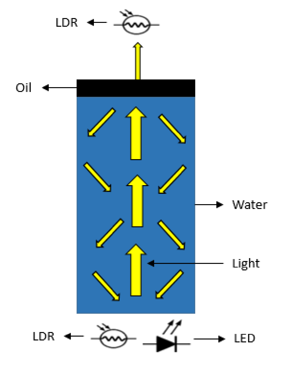
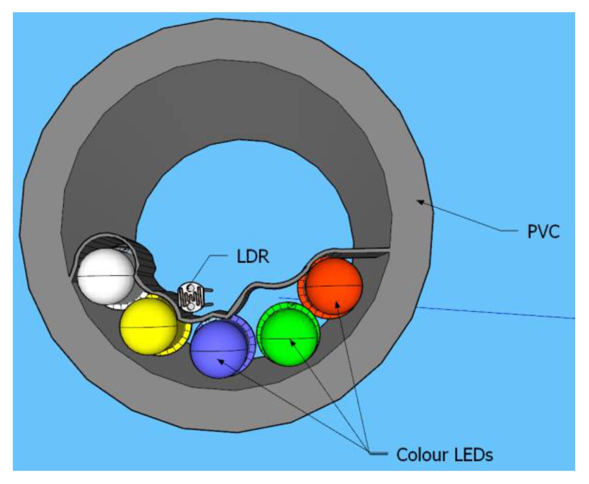
3.1. Description of the Optical System
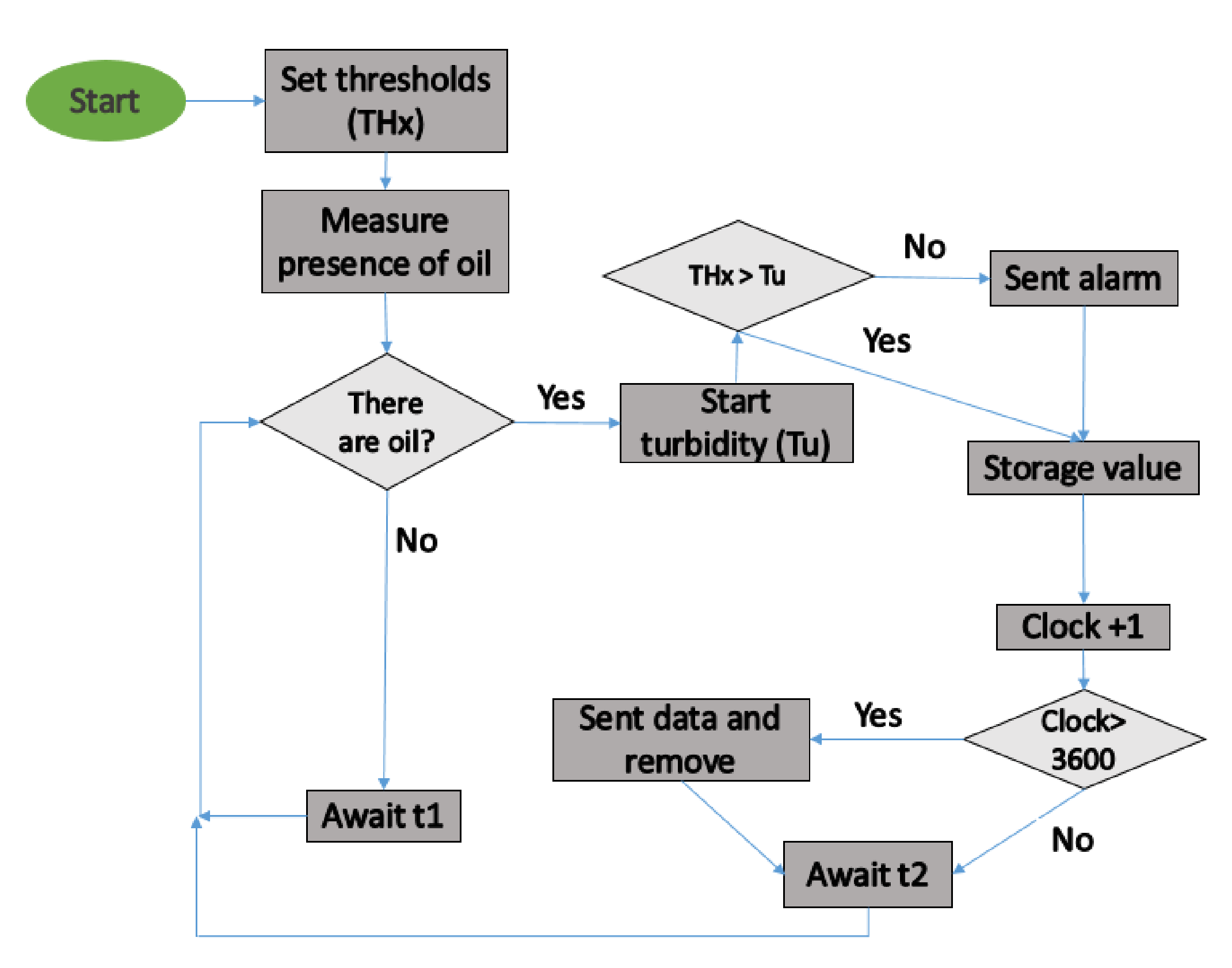
3.2. Operational Algorithm
4. Test Bench
4.1. Electronic Operation
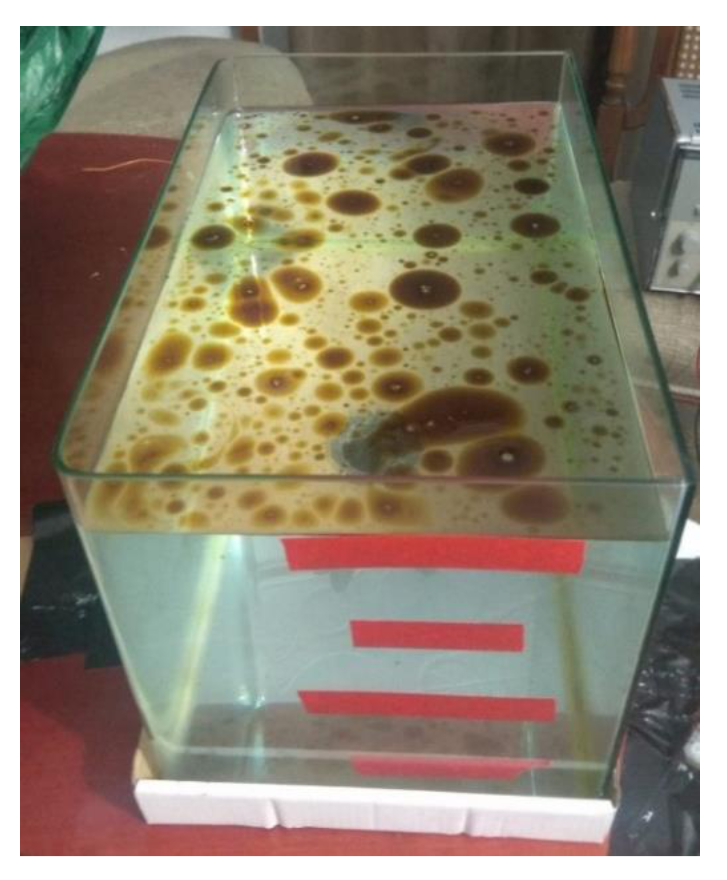
4.2. Sources of Oil
4.3. Samples for Calibration and Verification
5. Results
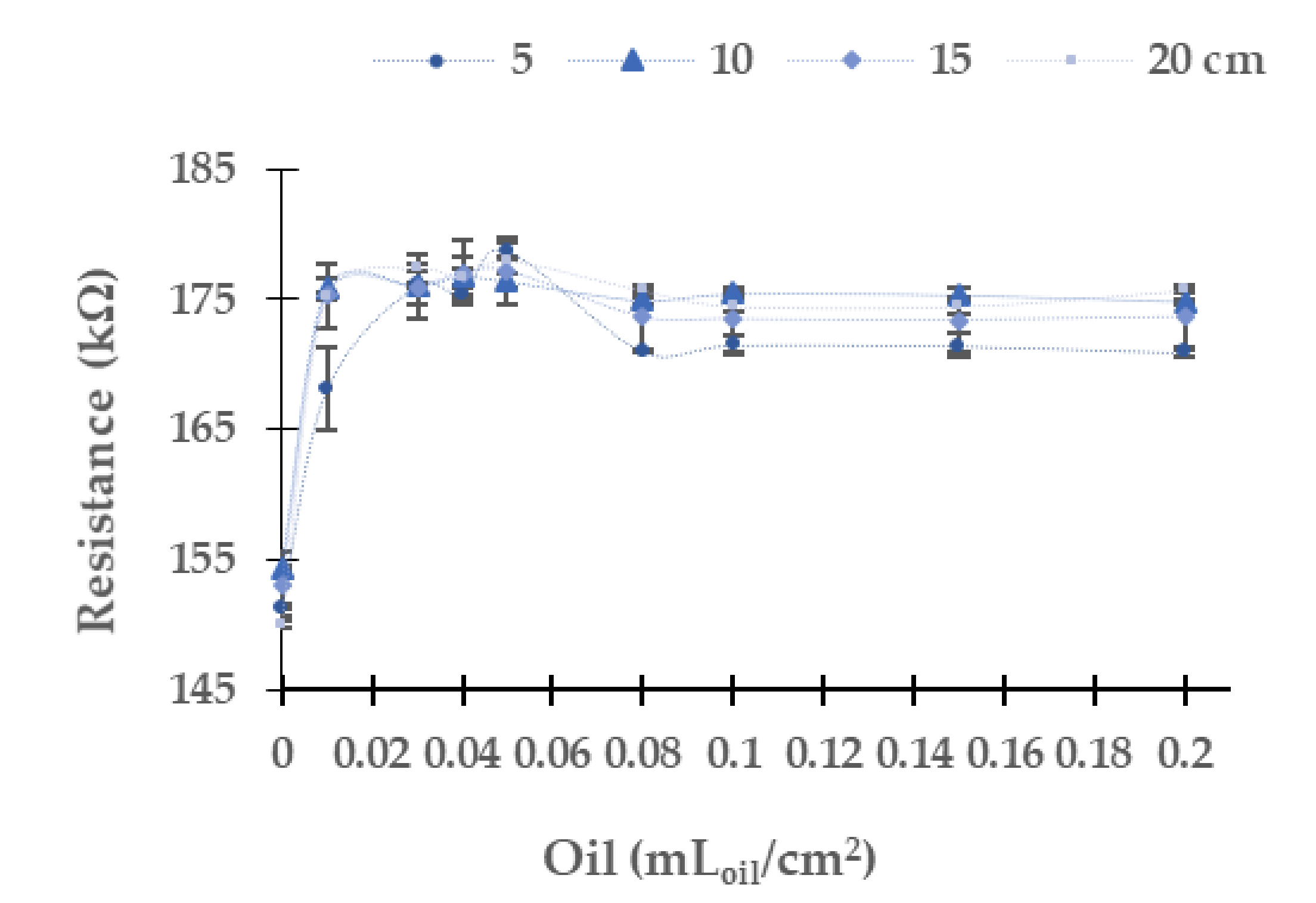
5.1. Industrial Oil of Diesel Engine
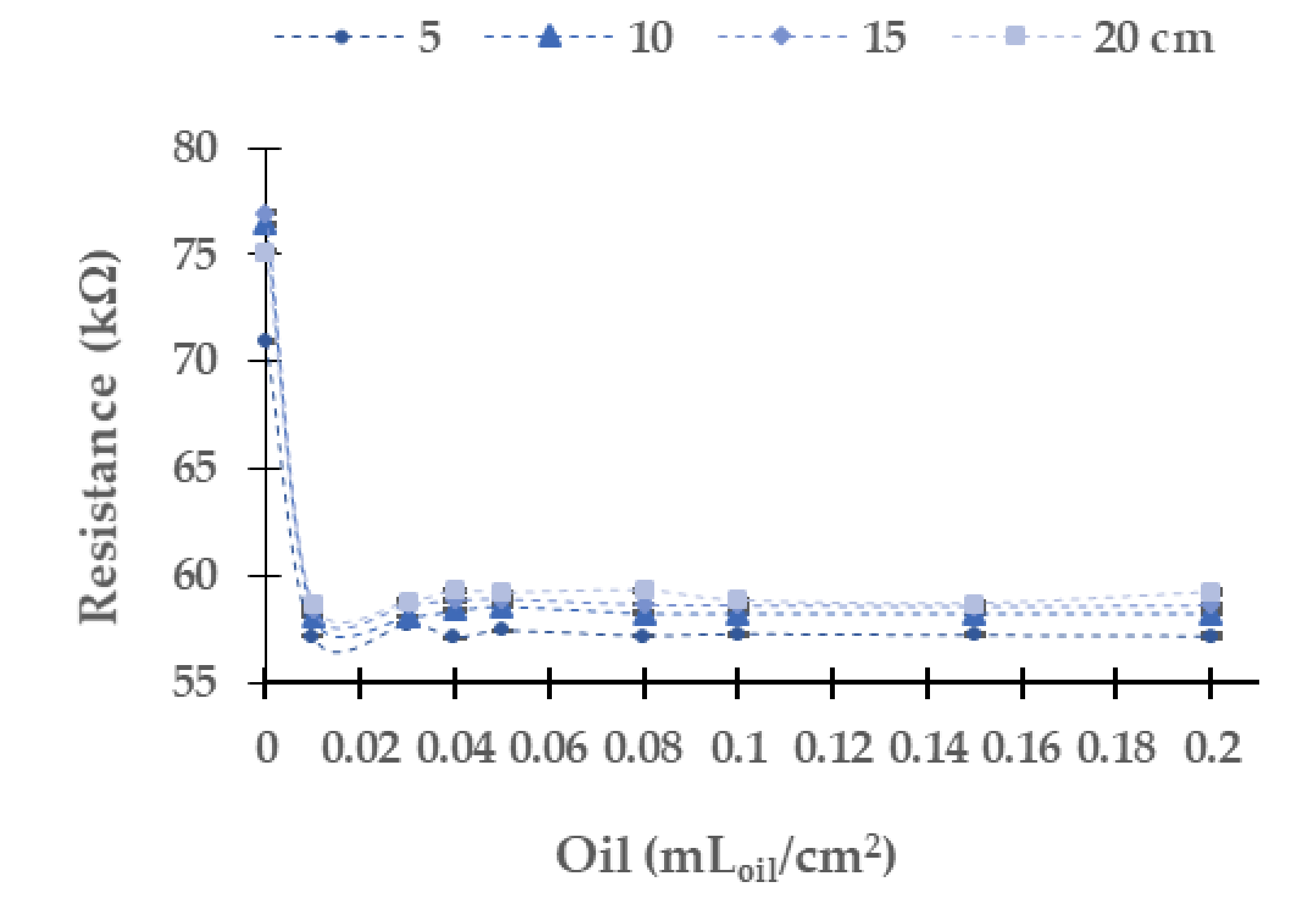
5.2. Industrial Oil of Gasoline Engine
5.3. Verification
6. Discussion
6.1. Differences among Oils
6.2. Selection of LEDs
6.3. Lessons Learned and Limitations of the Present Study
6.4. Relevance of the Present Study for Smart Irrigation and SMARTWATIR Project
7. Conclusions
Author Contributions
Funding
Institutional Review Board Statement
Informed Consent Statement
Data Availability Statement
Conflicts of Interest
References
- Bodirsky, B.L.; Rolinski, S.; Biewald, A.; Weindl, I.; Popp, A.; Lotze-Campen, H. Global Food Demand Scenarios for the 21st Century. PLoS ONE 2015, 10, e0139201. [Google Scholar] [CrossRef] [PubMed]
- KC, B.; Schultz, B.; Prasad, K. Water management to meet present and future food demand. Irrig. Drain. 2010, 60, 348–359. [Google Scholar] [CrossRef]
- Wu, X.; Zheng, Y.; Wu, B.; Tian, Y.; Han, F.; Zheng, C. Optimising conjunctive use of surface water and groundwater for irrigation to address human-nature water conflicts: A surrogate modeling approach. Agric. Water Manag. 2016, 163, 380–392. [Google Scholar] [CrossRef]
- Lopes, P.; Montagnolli, R.; Domingues, R.D.F.; Bidoia, E.D. Toxicity and Biodegradation in Sandy Soil Contaminated by Lubricant Oils. Bull. Environ. Contam. Toxicol. 2010, 84, 454–458. [Google Scholar] [CrossRef] [PubMed]
- Fujikura, M. Japan’s efforts against the illegal dumping of industrial waste. Environ. Policy Gov. 2011, 21, 325–337. [Google Scholar] [CrossRef]
- Hanley, N.; Johansson, P.O.; Kriström, B. Environmental cost-benefit analysis and water quality management. In Modern Cost–Benefit Analysis of Hydropower Conflicts; Edward Elgar Publishing: Jottham College, UK, 2011; pp. 6–21. [Google Scholar]
- Zhang, Q. Precision Agriculture Technology for Crop Farming; Taylor & Francis: Abingdon, UK, 2016. [Google Scholar]
- Peterson, S.H.; Roberts, D.A.; Beland, M.; Kokaly, R.; Ustin, S.L. Oil detection in the coastal marshes of Louisiana using MESMA applied to band subsets of AVIRIS data. Remote. Sens. Environ. 2015, 159, 222–231. [Google Scholar] [CrossRef]
- Nezhad, M.M.; Groppi, D.; Laneve, G.; Marzialetti, P.; Piras, G. Oil spill detection analysing “Sentinel 2” satellite images: A Persian Gulf case study. In Proceedings of the 3rd World Congress on Civil Structural, and Environmental Engineering, Budapest, Hungary, 8–10 April 2018; pp. 1–8. [Google Scholar]
- Taravat, A.; Del Frate, F. Development of band rationing algorithms and neural networks to detection of oil spills using Landsat ETM+ data. EURASIP J. Adv. Signal Process. 2012, 2012, 107. [Google Scholar] [CrossRef]
- Zhao, J.; Temimi, M.; Ghedira, H.; Hu, C. Exploring the potential of optical remote sensing for oil spill detection in shallow coastal waters-a case study in the Arabian Gulf. Opt. Express 2014, 22, 13755–13772. [Google Scholar] [CrossRef] [PubMed]
- Pisano, A.; Bignami, F.; Santoleri, R. Oil Spill Detection in Glint-Contaminated Near-Infrared MODIS Imagery. Remote Sens. 2015, 7, 1112–1134. [Google Scholar] [CrossRef] [Green Version]
- Salberg, A.-B.; Rudjord, O.; Solberg, A.H.S. Oil Spill Detection in Hybrid-Polarimetric SAR Images. IEEE Trans. Geosci. Remote Sens. 2014, 52, 6521–6533. [Google Scholar] [CrossRef]
- Ding, Y.; Wang, S.; Li, J.; Chen, L. Nanomaterial-based optical sensors for mercury ions. Trac Trends Anal. Chem. 2016, 82, 175–190. [Google Scholar] [CrossRef]
- Parra, L.; Rocher, J.; Escrivá, J.; Lloret, J. Design and development of low cost smart turbidity sensor for water quality monitoring in fish farms. Aquac. Eng. 2018, 81, 10–18. [Google Scholar] [CrossRef]
- Hübner, M.; Minceva, M. Microfluidics approach for determination of the miscibility gap of multicomponent liquid-liquid systems. Exp. Therm. Fluid Sci. 2019, 112, 109971. [Google Scholar] [CrossRef]
- Ramírez-Miquet, E.E.; Perchoux, J.; Loubière, K.; Tronche, C.; Prat, L.; Sotolongo-Costa, O. Optical Feedback Interferometry for Velocity Measurement of Parallel Liquid-Liquid Flows in a Microchannel. Sensors 2016, 16, 1233. [Google Scholar] [CrossRef] [PubMed] [Green Version]
- McCue, R.; Walsh, J.; Walsh, F.; Regan, F. Modular fibre optic sensor for the detection of hydrocarbons in water. Sens. Actuators B Chem. 2006, 114, 438–444. [Google Scholar] [CrossRef]
- Péron, O.; Rinnert, E.; Lehaitre, M.; Crassous, P.; Compère, C. Detection of polycyclic aromatic hydrocarbon (PAH) compounds in artificial seawater using surface-enhanced Raman scattering (SERS). Talanta 2009, 79, 199–204. [Google Scholar] [CrossRef] [PubMed]
- Albuquerque, J.S.; Pimentel, M.F.; Silva, V.L.; Raimundo, I.M.; Rohwedder, J.J.R.; Pasquini, C. Silicone Sensing Phase for Detection of Aromatic Hydrocarbons in Water Employing Near-Infrared Spectroscopy. Anal. Chem. 2005, 77, 72–77. [Google Scholar] [CrossRef] [PubMed]
- Yeh, P.; Yeh, N.; Lee, C.-H.; Ding, T.-J. Applications of LEDs in optical sensors and chemical sensing device for detection of biochemicals, heavy metals, and environmental nutrients. Renew. Sustain. Energy Rev. 2016, 75, 461–468. [Google Scholar] [CrossRef]
- Parra, L.; Sendra, S.; Lloret, J.; Mendoza, J. Low Cost Optic Sensor for Hydrocarbon Detection in Open Oceans. In Instrumentation Viewpoint; Universitat Politècnica de Catalunya: Barcelona, Spain, 2015; p. 45. [Google Scholar]
- Basterrechea, D.A.; Rocher, J.; Parra, L.; Lloret, J. Development of Inductive Sensor for Control Gate Opening of an Agricultural Irrigation System. In Proceedings of the 2020 Fifth International Conference on Fog and Mobile Edge Computing (FMEC), Paris, France, 20–23 April 2020; pp. 250–255. [Google Scholar] [CrossRef]
- Rocher, J.; Parra, M.; Parra, L.; Sendra, S.; Lloret, J.; Mengual, J. A Low-Cost Sensor for Detecting Illicit Discharge in Sewerage. J. Sens. 2021, 2021, 1–16. [Google Scholar] [CrossRef]
- Onda Radio ARISTON. Available online: https://www.ariston.es/producto/fac662b-promax-fuente-alimentacion-14958.aspx (accessed on 2 February 2021).
- TENMA. 2021. Available online: http://www.farnell.com/datasheets/1993717.pdf?_ga=2.177994341.1755120939.1591014303-1928794037.1591014303 (accessed on 21 January 2021).
- Agocs, A.; Budnyk, S.; Frauscher, M.; Ronai, B.; Besser, C.; Dörr, N. Comparing oil condition in diesel and gasoline engines. Ind. Lubr. Tribol. 2020, 72, 1033–1039. [Google Scholar] [CrossRef]
- Statgraphics. 2020. Available online: https://www.statgraphics.com/ (accessed on 21 January 2021).


| p-Value for Height | p-Value for Concentration | |
|---|---|---|
| Yellow | 0.0031 *** | <0.0001 *** |
| Red | 0.0006 *** | <0.0001 *** |
| Blue | <0.0001 *** | <0.0001 *** |
| Green | <0.0001 *** | <0.0001 *** |
| White | 0.0107 *** | <0.0001 *** |
| p-Value for Height | p-Value for Concentration | |
|---|---|---|
| Yellow | <0.0001 *** | 0.0977 |
| Red | 0.0003 *** | <0.0001 *** |
| Blue | <0.0001 *** | <0.0001 *** |
| Green | <0.0001 *** | <0.0001 *** |
| White | <0.0001 *** | <0.0001 *** |
| Height (cm) | Concentration (mLoil/cm2) | Calculated Concentration (mLoil/cm2) | AE (mLoil/cm2) | RE (%) |
|---|---|---|---|---|
| 10 | 0.02 | 0.025 | 0.005 | 27.1 |
| 10 | 0.06 | 0.073 | 0.013 | 21.1 |
| 10 | 0.12 | 0.134 | 0.014 | 11.5 |
| 15 | 0.02 | 0.020 | 0.000 | 2.3 |
| 15 | 0.06 | 0.079 | 0.019 | 30.9 |
| 15 | 0.12 | 0.111 | 0.009 | 7.9 |
| 20 | 0.02 | 0.019 | 0.001 | 2.7 |
| 20 | 0.06 | 0.073 | 0.013 | 22.0 |
| 20 | 0.12 | 0.110 | 0.010 | 8.5 |
| Colour | Gasoline | Diesel | ||
|---|---|---|---|---|
| Minimum (kΩ) | Maximum (kΩ) | Minimum (kΩ) | Maximum (kΩ) | |
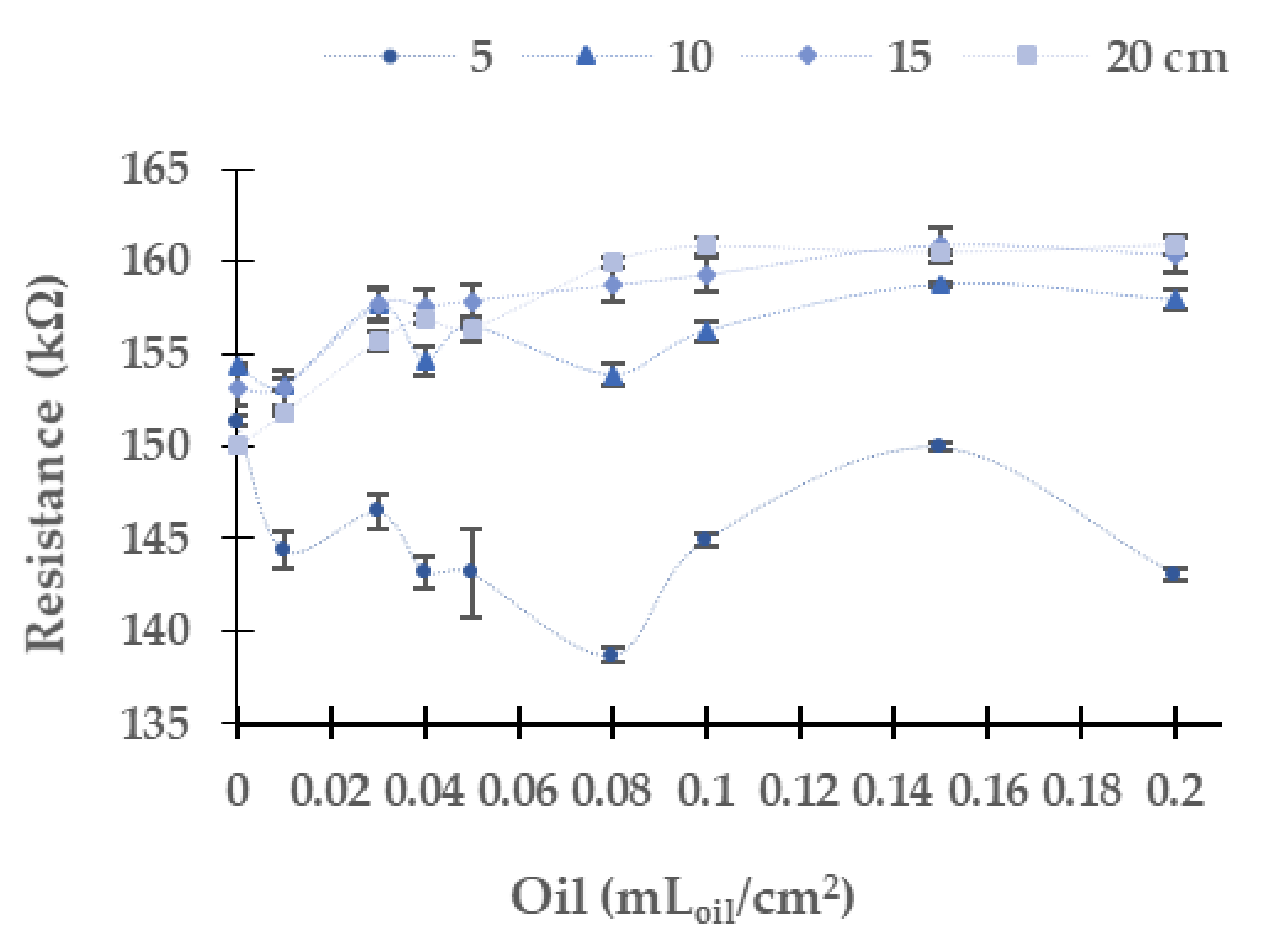
| Yellow | 138.68 | 160.91 | 150.01 | 178.81 |
| Red | 239.5 | 318.83 | 256.97 | 359.19 |
| Blue | 70.56 | 80.66 | 57.09 | 76.94 |
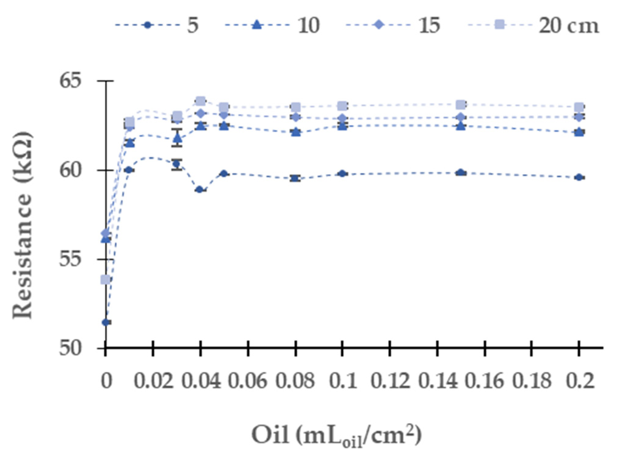
| Green | 50.88 | 65.57 | 51.44 | 63.85 |
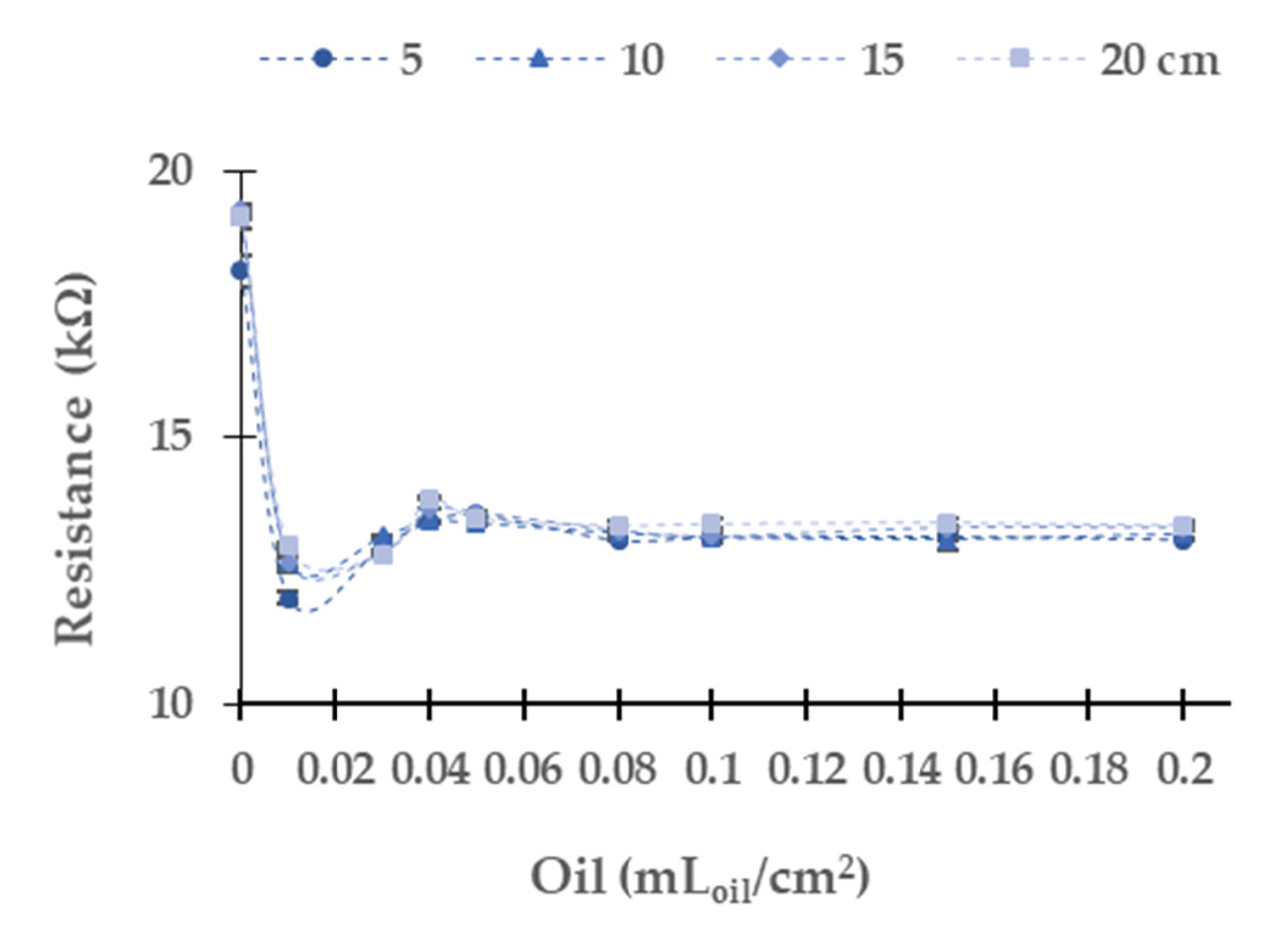
| White | 10.35 | 19.29 | 11.98 | 19.29 |
Publisher’s Note: MDPI stays neutral with regard to jurisdictional claims in published maps and institutional affiliations. |
© 2021 by the authors. Licensee MDPI, Basel, Switzerland. This article is an open access article distributed under the terms and conditions of the Creative Commons Attribution (CC BY) license (https://creativecommons.org/licenses/by/4.0/).
Share and Cite
Basterrechea, D.A.; Rocher, J.; Parra, L.; Lloret, J. Low-Cost System Based on Optical Sensor to Monitor Discharge of Industrial Oil in Irrigation Ditches. Sensors 2021, 21, 5449. https://doi.org/10.3390/s21165449
Basterrechea DA, Rocher J, Parra L, Lloret J. Low-Cost System Based on Optical Sensor to Monitor Discharge of Industrial Oil in Irrigation Ditches. Sensors. 2021; 21(16):5449. https://doi.org/10.3390/s21165449
Chicago/Turabian StyleBasterrechea, Daniel A., Javier Rocher, Lorena Parra, and Jaime Lloret. 2021. "Low-Cost System Based on Optical Sensor to Monitor Discharge of Industrial Oil in Irrigation Ditches" Sensors 21, no. 16: 5449. https://doi.org/10.3390/s21165449
APA StyleBasterrechea, D. A., Rocher, J., Parra, L., & Lloret, J. (2021). Low-Cost System Based on Optical Sensor to Monitor Discharge of Industrial Oil in Irrigation Ditches. Sensors, 21(16), 5449. https://doi.org/10.3390/s21165449