Article

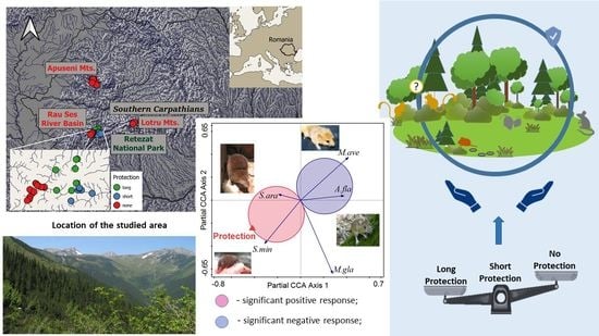
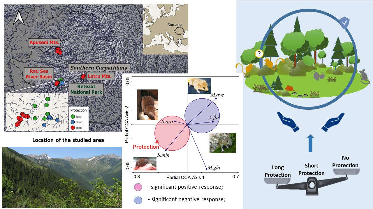
Effects of Long-Term Habitat Protection on Montane Small Mammals: Are Sorex araneus and S. minutus More Sensitive Than Previously Considered?

by
Ana Maria Benedek
1,*,
Anamaria Lazăr
2,
Niculina Viorica Cic
1,
Maria Denisa Cocîrlea
1 and
Ioan Sîrbu
1
1
Faculty of Sciences, Lucian Blaga University of Sibiu, 5-7 Raţiu Street, 550012 Sibiu, Romania
2
Department for Engineering and Management in Food and Tourism, Faculty of Food and Tourism, Transilvania University of Brașov, 148 Castelului Street, 500036 Braşov, Romania
*
Author to whom correspondence should be addressed.
Diversity 2022, 14(1), 38; https://doi.org/10.3390/d14010038
Submission received: 24 November 2021 / Revised: 4 January 2022 / Accepted: 5 January 2022 / Published: 8 January 2022
(This article belongs to the Special Issue Advances in Diversity and Conservation of Terrestrial Small Mammals)

Abstract

:
Protection of natural areas by restricting human activities aims to preserve plant and animal populations and whole communities, ensuring the conservation of biological diversity and enhancement of ecosystem services. Therefore, it is expected that the longer the protection, the stronger the desired effects. We evaluated the responses of small mammals at the population and community levels under protection in the southern Carpathian Mountains. We surveyed small mammals for five years in sites with long- and short-term protection and non-protected. Besides protection status, we included elevation, habitat heterogeneity, and the month of survey as predictors in our models. As response variables, we considered abundance, presence, species composition and species richness. Community abundance responded to all four predictors and species composition was influenced by protection status and month of study. The shrews Sorex araneus and S. minutus had positive responses to protection, both in terms of abundance and relative abundance (their ratio within the community). Our results suggest that overall, montane small mammal communities respond positively to long-term protection, especially S. araneus and S. minutus. These shrew species are considered habitat generalists, but they appear to be in fact sensitive to the habitat quality enhanced through protection.

Graphical Abstract

1. Introduction

The primary causes of decline in global biodiversity are the destruction and degradation of natural ecosystems [1,2]. Forests have one of the longest histories of aggressive human intervention, especially in densely populated areas [3]. For a long time, forests were completely removed because of the need for timber [4] and for expanding pastures [5], agricultural fields and settlements [4], while later management practices included a variety of actions for enhancing forest regeneration [6]. Consequently, most contemporary forests of Europe are monoculture plantations of intensive commercial forestry [7]. Although various nature-friendly management methods have been developed and applied within organized forestry in the last 300 years [7], only a small proportion of the European woodland area remains spared of human impact, mostly in montane areas. Because of their inaccessibility, low human population densities and economic underdevelopment, the Romanian Southern Carpathian Mountains still host an important part of the European virgin forests [7], but these lack strict protection [8].
Protected areas are major evidence of humanity’s efforts toward maintaining biodiversity [9]. Most of the time, a well-managed protected area reduces habitat loss and maintains population levels, even for threatened species [10]. For example, Gray et al. [11] found that species richness is 10.6% and abundance is 14.5% higher in protected areas than in non-protected ones, this being the result of differential land use between the two types of areas. Recently, protected areas have been created not only to conserve unique landscapes and ensure habitats for endangered species but also to contribute to sustaining human communities and, among other functions, to adapt to climate changes [10].
Small mammals are an essential component of woodland ecosystems, where they are usually abundant and perform important ecological functions, including bioturbation [12,13,14,15], seed [16,17,18] and fungus [19,20,21] dispersal, and arthropod predation [22,23,24]. They are also one of the main food sources for birds of prey, mammalian predators and even reptiles [12,25,26,27]. Therefore, changes in their population densities might have cascading effects on forest ecosystem structure and functions [12,28].
Studies focused on the response of small mammals to a particular human impact, such as the Peru LNG pipeline [29] or the clearings in managed Central European forests [12,30,31,32,33], have shown that small mammals may also be useful indicators of environmental change, responding rapidly to changes in woodland management [29,30]. Therefore, it is expected that habitat protection would positively affect small mammal communities, with differential responses of various species, depending on their ecological requirements.
Numerous studies on small mammals have been conducted in various protected areas, such as wet meadows or riparian forests [34], wooded urban areas [35] and forests [36]. Some studies aimed to compare small mammal abundances and diversities within and outside protected areas [37,38]. However, to the best of our knowledge, no studies have tested the effect of long-term protection on small mammals in mountain landscapes.
We sought to assess the response of small mammals to the duration of habitat protection in mountain landscapes. We assessed small mammal responses to short- and long-term protection in montane habitats at community and population levels. Because natural habitats tend to be more complex than human-altered ones, the lack of protection may affect animal communities by diminishing habitat heterogeneity; therefore, we included this variable in our models. We also considered elevation and the month of study because we expected a significant elevational pattern and seasonality in the small mammal community parameters. Thus, we examined relationships between species abundance or presence, total abundance, species composition, and richness of small mammals as response variables and protection duration, habitat heterogeneity, elevation and month as explanatory variables. We predicted an overall positive effect of duration of forest protection on small mammal abundance and richness, independent of habitat heterogeneity.

2. Materials and Methods

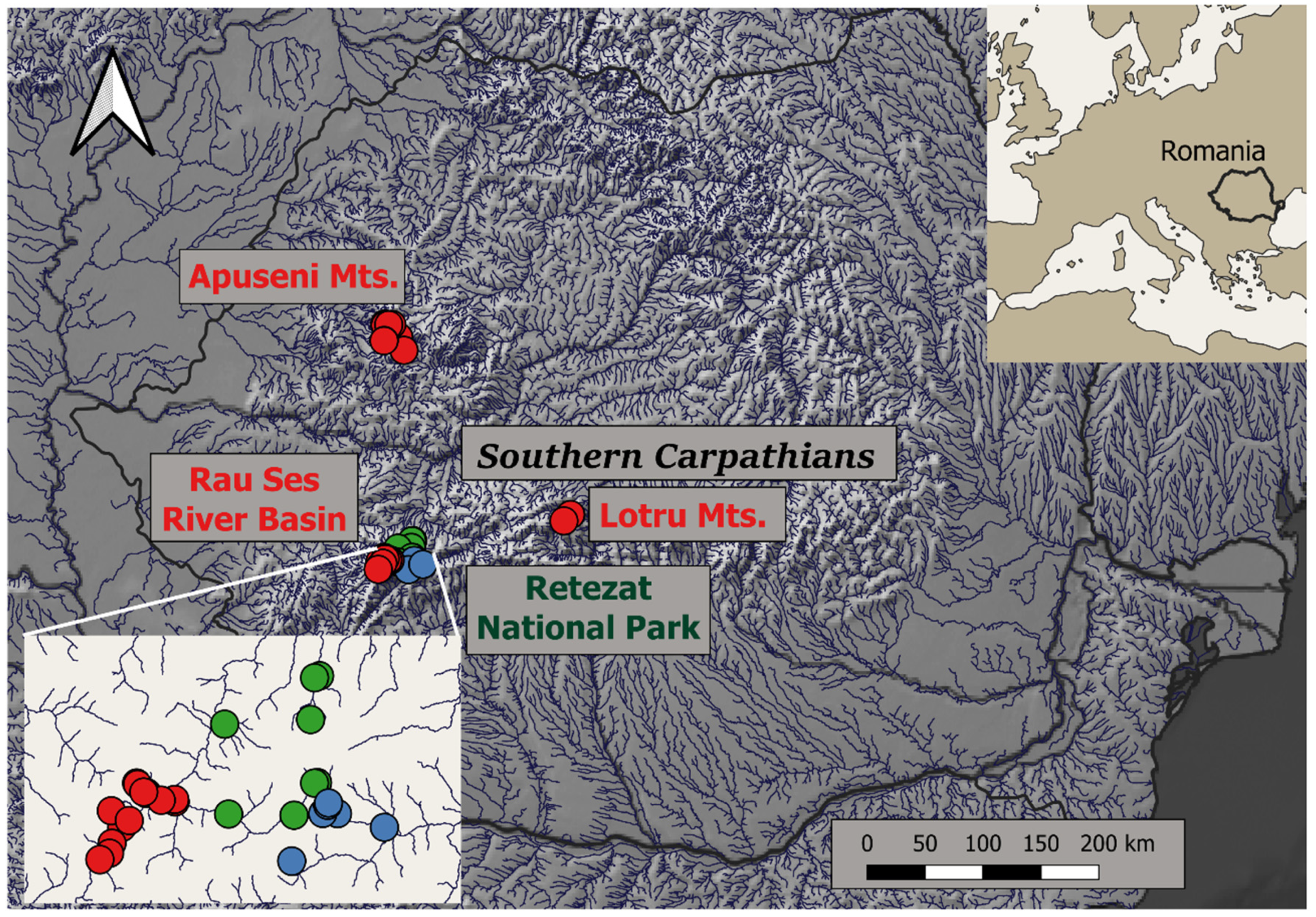
2.1. Description of the Study Areas

We conducted our study in four areas of the Carpathian Mountains (Romania): Apuseni Mountains, Lotru Mountains, Râu Șes River Basin and Retezat Mountains (Figure 1).
The Apuseni Mountains, the northernmost of the study areas, are characterized by low elevations (the highest peak is 1849 m a.s.l.). Covered in forests, with no subalpine shrubs or meadows and with scattered settlements, these mountains have a long history of logging, with many plantations and artificially thinned forests, clearings, hayfields and pastures. Although the study sites were part of the Apuseni Nature Park (established in 1990) at the time of survey, the recent and ongoing human disturbance (mainly forest exploitation) was very intense throughout the park, including in the near vicinity of some of our trapping sites.
The Lotru Mountains have been intensely logged during the last century. As a result, most forest plots are secondary forests, either planted or naturally regenerated. In some places, spruce forests were planted below their natural elevation. During the study period, no logging occurred in the trapping sites or nearby.
The Râu Șes River Basin (including parts of Țarcu and Godeanu Mountains) comprises a mix of virgin, natural and planted forests, and subalpine shrubs and meadows. Old exploitations affected most of the spruce forests, which were clear-cut and then replanted, but forests at the timberline were usually kept intact. Beech and mixed forests were exploited by clear-cut or felling of mature trees. Tree trunks were removed while branches were usually left in place, representing most of the coarse woody debris in logged forest plots.
The Retezat Mountains are one of the tallest mountain ranges in Romania (the highest peak is 2509 m a.s.l.), with extensive high ridges and peaks and include Retezat National Park, the oldest protected area in Romania, founded in 1935. In 1979, it was declared a Biosphere Reserve and included in the UNESCO World Heritage. After the change of the political regime in 1989, the number of protected areas in Romania increased greatly, and in the 1990s, the size of Retezat National Park was also increased by including areas adjacent to the limits of the early park.
In these areas, we surveyed forested habitats. At lower elevations, there are mainly beech (Fagus sylvatica) forests, usually with a dense tree canopy but poor herbaceous layer and understory. Mixed forests, composed of differing proportions of beech and Norway spruce (Picea abies) with scattered silver fir (Abies alba) and sycamore (Acer pseudoplatanus), are characteristic of mid-elevations. A Norway spruce forest belt reaches up to the timberline, which usually is present at elevations between 1600 and 1800 m, depending on slope exposure and other geomorphlogical characteristics of the site. The cover of shrub and herbaceous layers varies greatly in spruce forests, the understory being composed mainly of spruce saplings, often with blueberry (Vaccinium myrtillus) bushes and a thick moss layer. The tree canopy cover of spruce forests decreases near the timberline, but the herbaceous layer is also reduced due to rocky outcrops and surfacing stones. At the timberline, mountain-ash (Sorbus aucuparia), stone pine (Pinus cembra) and juniper (Juniperus communis) shrubs are interspersed among dwarf spruce trees. This natural elevational succession of forest habitats is sometimes altered by temperature inversions or past logging and reforestation, which artificially lowered the lower limit of spruce forests.

2.2. Protection Status and Habitat Variables

We coded the protection status of the trapping areas as an ordinal variable, based on the duration of protection as: 2—sites benefitting from long-term protection (within the borders of the early Retezat National Park), 1—sites with short-term protection (in areas included in the park after 1989), and 0—sites in unprotected areas (here we also included the Apuseni Mountains) (Figure 1).
Because trapping was conducted in forested habitats, we expressed habitat heterogeneity based on five forest features evaluated for each transect using ordinal variables on a scale from 1 to 4, as follows: for tree canopy diversity: 1—only one species, 2—one dominant species (over 75% cover), 3—two dominant species (over 40% cover each) and 4—three or more codominant species. For cover of the shrub canopy: 1—no shrubs, 2—<20% shrub cover, 3—21–40% shrub cover and 4—41–60% shrub cover. For cover of the herb layer: 1—0–25% herb cover, 2—26–50% herb cover, 3—51–75% herb cover and 4—76–100% herb cover. For abundance of coarse woody debris: 1—absent, 2—scarce, 3—moderate and 4—abundant and rocky outcrops. For surfacing stones: 1—absent, 2—scarce, 3—moderate and 4—abundant. We calculated habitat heterogeneity as the geometric mean of these five variables. We chose the geometric mean over the arithmetic mean to give more weight to more equal contributions of the five elements determining heterogeneity. We also considered the elevation (between 820 and 1910 m a.s.l.) of each surveyed habitat both as a quantitative variable (expressed in km for similar scaling with the other variables) and a factor with three levels (low—<1150 m, medium—1150–1450 m, high—>1450 m) because in some response variables, we expected a unimodal response with a maximum at mid-elevation.
Small mammal trapping was conducted during the warm season (from June to September), and the month of survey was considered an ordinal variable: 1—June, 2—July, 3—August, 4—September.
To avoid multicollinearity, we tested the correlation between our four predictors prior to model construction, using the non-parametric (because of the ordinal variables) Spearman correlation. The only two variables that showed a significant correlation (p = 0.008) were protection status and elevation, but the correlation coefficient was low (rho = 0.3); therefore, we kept all the predictors in the analyses. In addition, we tested for multicollinearity of the multiple models using the variance inflation factor, but none was higher than 2, confirming no multicollinearity of predictors.

2.3. Small Mammal Trapping

Between 2003 and 2007, we conducted several trapping sessions using artisanal wooden and plastic box-traps (18 × 10 × 8 cm) set in transects. Transects included 30 to 40 live traps set 15 m apart, along the contour lines and parallel to the closest watercourse, forest edge, road or trail, within homogenous habitats. Trapping sites were selected along several valleys to cover the elevational gradient of forested habitats in the Retezat National Park and at similar elevations in the non-protected areas. In total, we surveyed 39 habitats, 25 in non-protected areas (1 broadleaved forest, 11 mixed, 13 spruce), 6 in newly protected areas (2 broadleaved, 2 mixed, 2 spruce) and 8 in the early park (1 broadleaved, 2 mixed, 5 spruce). Habitats were randomly surveyed between one and five times (once each year), resulting in 75 transects (visits), 34 in non-protected areas (1 broadleaved, 18 mixed, 15 spruce), 24 in newly protected areas (7 broadleaved, 7 mixed, 10 spruce) and 17 in the early park (3 broadleaved, 2 mixed, 12 spruce).
Traps were baited with sunflower seeds, apple slices and meat pasta. Hay was provided as bedding material. Traps were checked at dawn and dusk for two or three consecutive days, resulting in a trapping effort that varied between 60 and 120 trap nights (TN) per transect. Many traps were stolen, disturbed by animals (e.g., shepherd dogs, foxes, wild cats, squirrels) or closed by wind, heavy rain or invertebrates, mainly large coleopterans and slugs attracted by the bait. Therefore, to calculate the effective TN, we subtracted from the total number of TN those that were non-functional. The effective trapping effort varied between 20 (we eliminated the few transects where the effective effort was lower) and 120 TN per transect, with a total of 3657 TN. We identified captured animals to species based on morphological traits, and after marking, we released each animal at its trapping site. Because we were not interested in recaptures from one year to the next and only needed to identify recaptures during the same trapping session, we used temporary marking by fur clipping. We did not include recaptured individuals in any analysis.

2.4. Data Analysis

We used the following response variables: abundance, presence, species richness and species composition of small mammals. As a proxy for abundance, we used the number of captured individuals, but because the trapping effort strongly influences capture success, we also considered the number of effective TN. This was included in the models or used to calculate the capture index, as the number of captured individuals per 100 effective TN. As measures of species richness, we used the number of species captured per transect and the Chao estimator [41], calculated in the vegan package [42] in R version 3.6.1 [43]. To compare the overall diversity, we constructed the rarefaction curves for each protection status using the function iNEXT in the iNEXT package [44]. Because of the variation in sample size (different trapping efforts among transects), we used the individual-based approach for constructing rarefaction curves.
Some transects were surveyed repeatedly from year to year, but the strong temporal fluctuations in species abundance and spatial synchrony (at least at a local scale) [45] caused the effect of the site to be non-significant. Therefore, we accounted only for temporal dependency among transects, including year as a random factor when its effect was significant, using mixed-effects models in the lme4 package [46] in R. When the effect of year was not significant, we constructed (generalized) linear models ((G)LMs).
We modeled the total abundance and the abundance of the three dominant species of small mammals. We included the number of captured individuals as the response variable and the trapping effort as offset. Because overdispersion was significant, we used negative binomial generalized linear mixed models (GLMMs). For less abundant species (but only those captured in more than five transects), we constructed models of their presence using binomial GLMs (probability of presence did not vary significantly among years). Species richness (number of captured species and Chao estimator) followed the Gaussian distribution and did not show significant interannual variations; thus, we used LMs. To compare the models and find the most parsimonious one, we used the stepwise forward selection procedure (starting from the null model) with the likelihood-ratio test, which assesses the goodness of fit of two competing nested models based on the ratio of their likelihoods. In the GLMMs, the explained variation for the best model was expressed by the conditional and marginal pseudo-R2 statistics based on Nakagawa et al. [47], computed in the MuMIn package [48]. The marginal R2 represents the variance explained only by the fixed part of the model, while the conditional R2 is interpreted as the variance explained by the entire model, including both fixed and random factors. For the GLMs, we calculated the explained deviance, and for the LMs, the adjusted coefficient of determination (R2). The effects of interactions among predictors were also tested, but none were significant.
The effect of protection status and other variables at the community level was analyzed using Canoco 5.12 software [49]. We first ran a detrended correspondence analysis (DCA), and the length of the gradient was 3.2, suggesting the use of the unimodal method, canonical correspondence analysis (CCA). In the CCA, the response variables are the species’ ratios within the community (the relative abundances of species), which we refer to as species composition hereafter. In the partial CCA, the effect of the considered predictors on species composition is evaluated after removing the effect of a covariate, in our case, the year. Rare species (captured in less than five transects) were not included in the analyses. Response variables were log-transformed by the expression y’ = log(y + 1). The interactive forward selection was applied to choose the most parsimonious set of predictors for the partial CCA. Probabilities were adjusted (padj) to correct type-I error inflation caused by multiple testing, using the false discovery rate values [50]. The significance of ordination axes was tested by the Monte-Carlo permutation test with 999 permutations per test. Permutations were restricted to blocks defined by the year of survey.
The significance of the response of individual species to the selected predictors was illustrated through t-value biplots, which approximate the t-values of the regression coefficients of a multiple regression with the particular species as the response variable and all the habitat types as predictors, revealing statistically significant pairwise relationships between each response variable and each predictor [50].

3. Results

3.1. Trapping Results

During the 5 years of study, we trapped 343 individuals of 13 species (Table 1). The rodents Myodes glareolus (34.4% of the captured individuals, with the standard error of the mean percentage—SE = 2.5%) and Apodemus flavicollis (32.6%, SE = 2.5%), and the shrew Sorex araneus (23.6%, SE = 2.3%) were dominant.
Although the overall abundance of S. araneus (2.21 individuals/100 TN) was lower than that of A. flavicollis (3.06 individuals/100 TN), its frequency was higher; S. araneus was captured in 33 of the 75 transects (44%, SE = 5.7%), while A. flavicollis in 24 transects (32%, SE = 5.3%). Myodes glareolus had the highest frequency (57.3%, SE = 5.7%). Muscardinus avellanarius and Sorex minutus were captured in 8 (10.6%, SE = 3.5%) and 5 (6.7%, SE = 2.8%) transects, respectively, while the other 8 species were found in less than 5 transects. Trapping success varied between 0 and 92.6 individuals/100 TN, with a mean of 11.32 individuals/100 TN (SE = 1.7 individuals/100 TN). Species richness varied between zero and five species per transect, while the estimated number of species (Chao estimator) varied between zero and six.

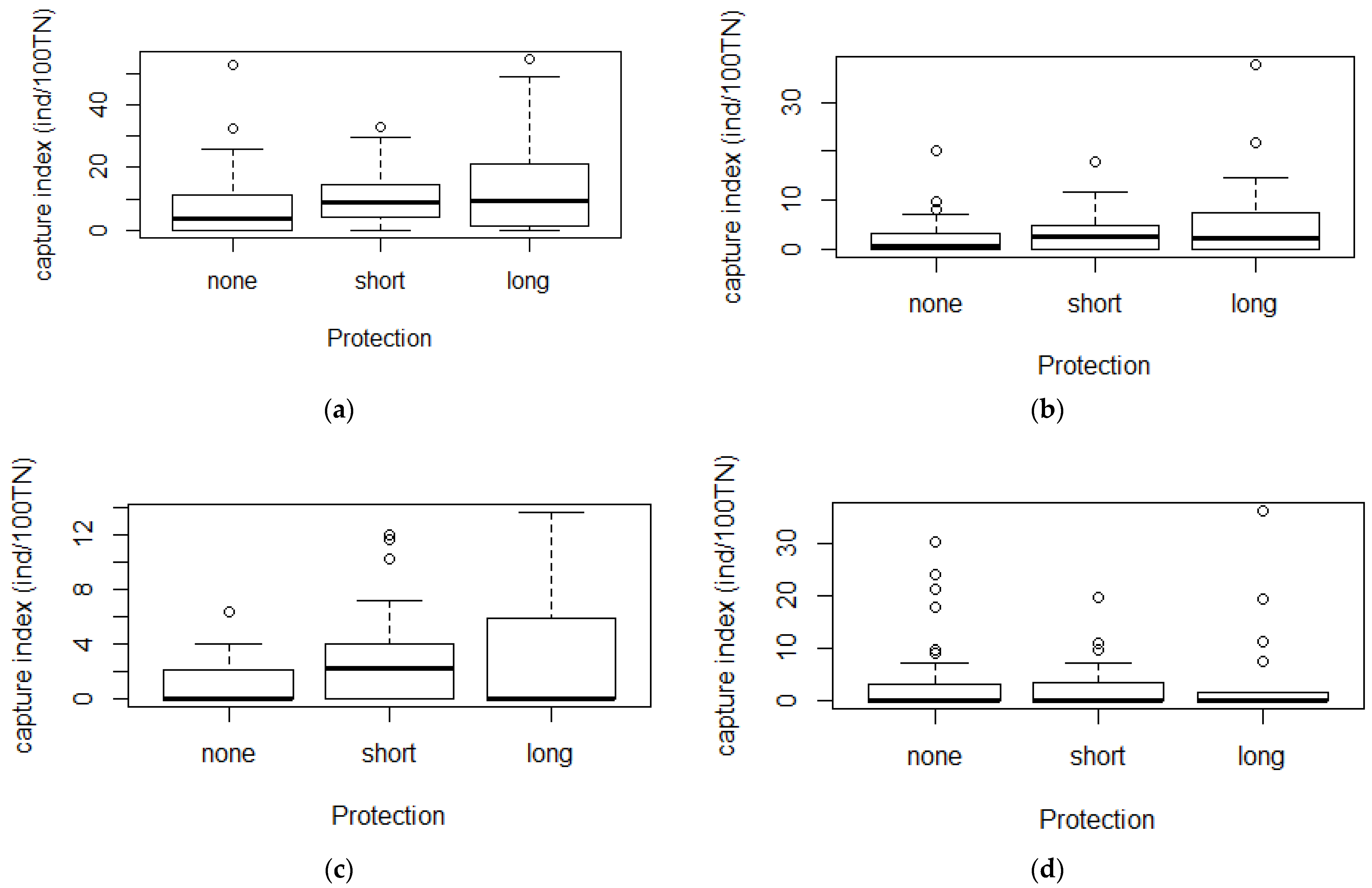
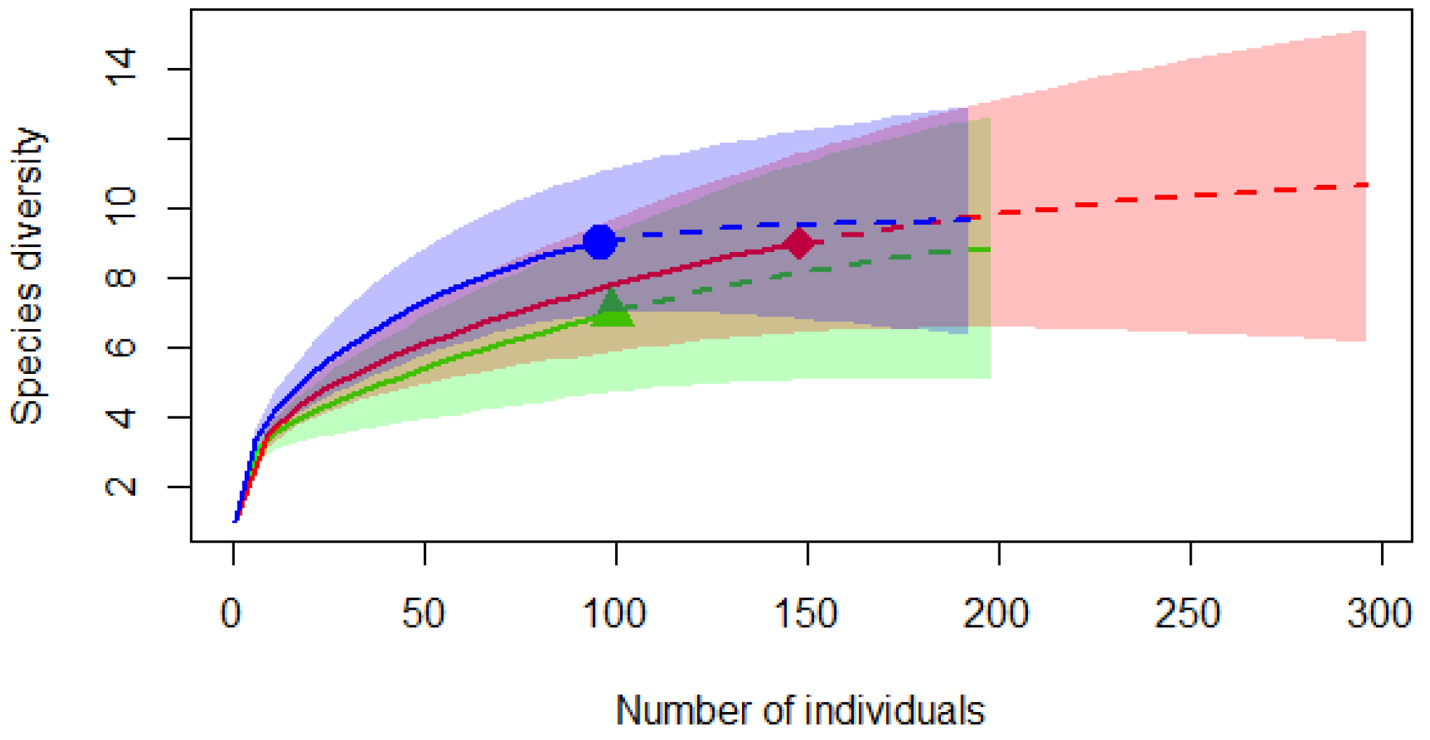
3.2. Effect of Long-Term Protection on Montane Small Mammals

The overall capture index increased slightly with the length of protection (Figure 2a) due to the higher abundances of M. glareolus (Figure 2b) and S. araneus in the protected areas. The median capture index of S. araneus in the long-term protected areas was zero because in most of the transects it was not captured, but when present, abundances were higher than in other areas (Figure 2c). Apodemus flavicollis had similar values in non-protected and short-term protected areas and lower values in long-term protected areas (Figure 2d).
When accounting for interannual variations and the effect of the other predictors (habitat heterogeneity, elevation and month of survey), in the mixed models with year as random factor, the protection status had a significant positive effect on the total abundance and of two dominant species, M. glareolus and S. araneus, but it did not influence A. flavicollis (Table 2).
Interannual variations in total abundance were very strong, with the pseudo-R2 for fixed effect component 0.204 of the 0.664 for the whole model. Total abundance also proved to be significantly affected by the other three predictors. There was an increase with habitat heterogeneity, from June to September and a decrease with elevation (Table 2). Myodes glareolus also showed significant interannual variation and a significant unimodal elevational pattern, with maximum abundances at medium elevations between 1150 and 1450 m a.s.l. and minimum abundances above 1450 m a.s.l (Table 2). Sorex araneus showed a significant seasonal pattern, with increasing abundances from June to September but no significant interannual variation. Variation among years was the strongest in A. flavicollis, for which year explained more variation in abundance than elevation and habitat heterogeneity, as the pseudo-R2 for the fixed effect component of the model was only 0.122 of the 0.772 for the whole model. Unlike M. glareolus, A. flavicollis had a linear, negative response to elevation and a positive response to habitat heterogeneity (Table 2).
The presence of the less abundant species, M. avellanarius and S. minutus, did not show significant interannual variations and were significantly affected by protection status (Table 2). The presence probability of S. minutus was positively affected by the duration of protection, and the explained deviance was 0.167. For M. avellanarius, the capture probability decreased with the duration of protection, but its effect was only marginally significant; therefore, the model fit was low (Table 2).
In contrast, species richness (observed and estimated) was not affected by the protection status but showed a significant seasonality, increasing from June to September. In addition, the captured number of species also showed significant interannual variation. However, the variation in species richness explained by these models was low (Table 2), which indicates that species richness is more dependent on other variables that were not included in the analyses, being beyond the scope of this paper.
Rarefaction curves (Figure 3) indicate that recently protected areas had the highest overall species richness, while in the early park, the species richness was the lowest. However, the large confidence intervals, caused by the high number of singletons and doubletons, show that a much larger sample size is needed to compare the species richness of areas with different protection statuses.

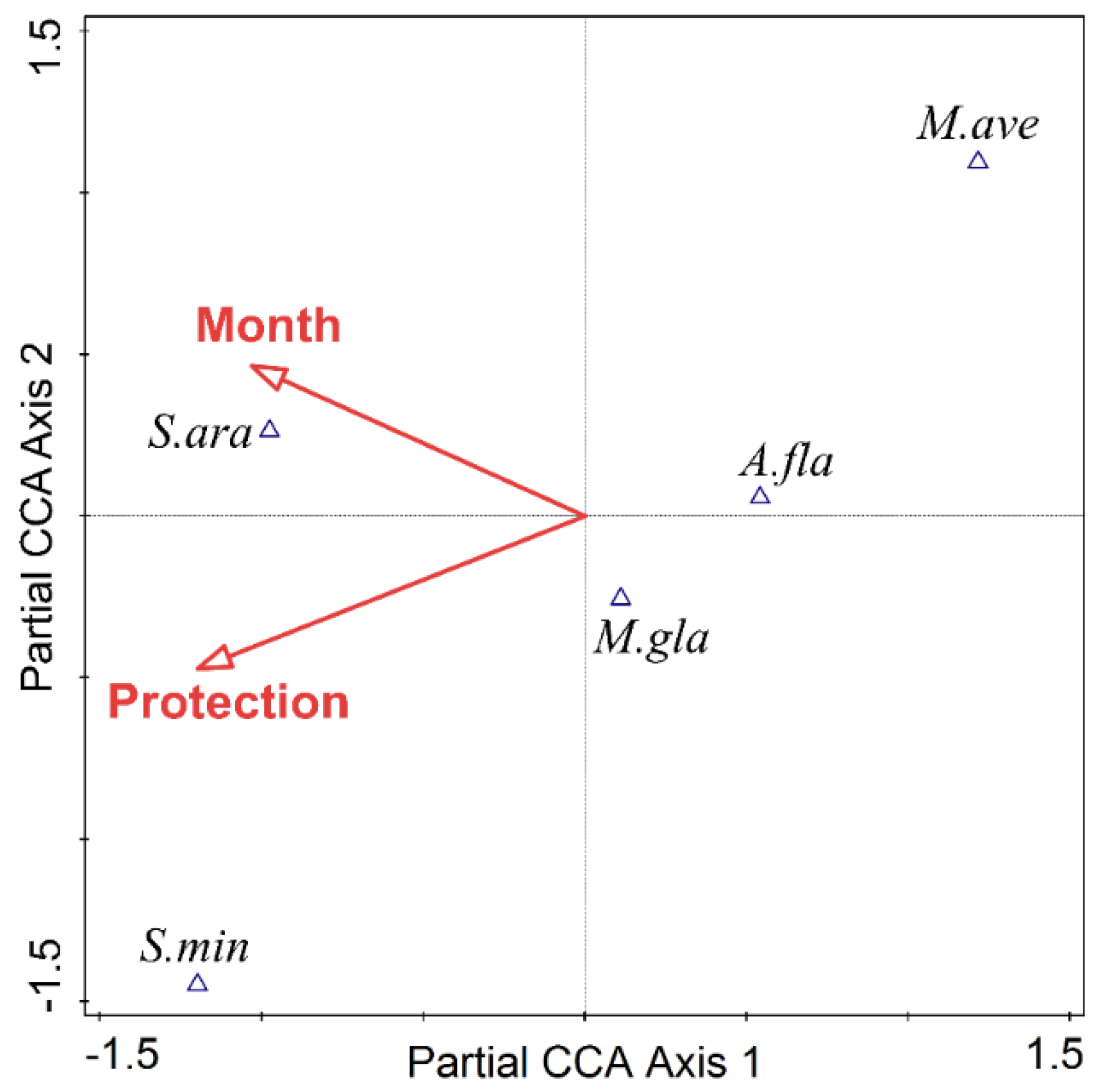
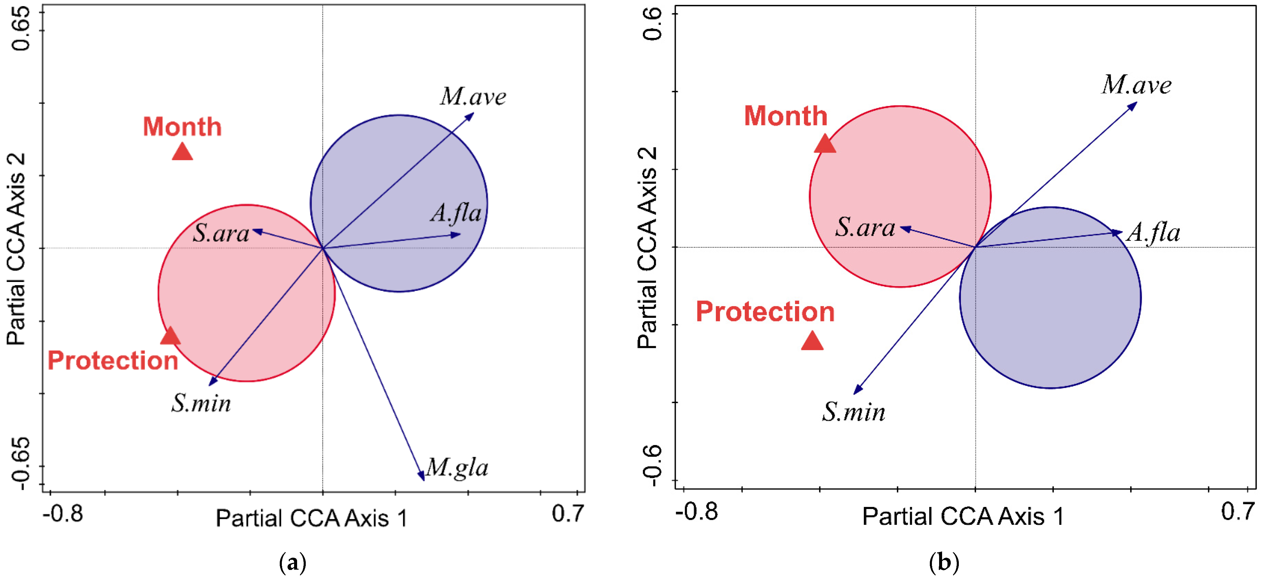
3.3. Responses of Small Mammal Species Composition

The variables that we considered were significant predictors of small mammal species composition (pseudo-F = 3.1, p = 0.002), explaining 19.5% (13.2% adjusted) of the partial variation in the community structure, i.e., after we removed the effect of year. All variables except habitat heterogeneity were significant predictors of community composition when considered separately, but their effects were partially overlapping. The best model, including protection status and month of study (pseudo-F = 4.7, p = 0.002), accounted for 15% (11.9% adjusted) of the residual variation in species composition after removing the effect of interannual fluctuations. The two predictors were mostly independent in the constrained ordination space. Duration of protection was positively associated with the relative abundance of S. minutus and S. araneus and negatively associated with that of M. avellanarius and A. flavicollis (Figure 4). The responses of S. araneus and A. flavicollis were significant, as shown by the t-value biplots (Figure A1a). The relative abundance of the two shrews increased from summer to autumn, while the relative abundance of the rodents decreased (Figure A1b), but only the response of S. araneus was significant (Figure A1b).
The interaction between protection status and month of survey had no significant effect on species composition (pseudo-F = 1.6, p = 0.136).

4. Discussion

We surveyed small mammal communities in protected and unprotected areas, in forest habitats differing in elevation and heterogeneity. Our study is the first to evaluate the response of small mammal communities to the duration of habitat protection in a montane landscape along an elevational gradient, at least in central Europe. During our survey, we identified 13 species. Myodes glareolus, Apodemus flavicollis and Sorex araneus were dominant. All four predictors that we tested (protection duration, habitat heterogeneity, elevation and month of survey) affected one or several of our response variables (species and total abundance, species presence, species richness and composition), but none had a significant effect on all of them.

4.1. Effects of Habitat Protection Status

The abundances of M. glareolus, S. araneus and S. minutus increased significantly with protection duration, as did the total abundance (Table 2). The usual ratio of shrews within small mammal communities is between 8–15% [34]. This value is low compared with the overall relative abundance of S. araneus in our study (23.6%) and especially with the value for the early park (35.5%). These values are uncommonly high for S. araneus [51], especially considering that we used box-traps for sampling, which usually underestimate the abundance of shrews [52,53]. The increase of S. araneus population abundances due to habitat protection [35] and the decrease due to forest management [54] were previously reported.
Sorex araneus and S. minutus are euryoecious species populating both lowlands and high areas [55]. The abundance of invertebrate communities is one of the most important microhabitat characteristics for shrews [23]. In harsh conditions, such as montane habitats, the spatial and trophic niches of S. araneus and S. minutus overlap [56], which is probably why the two species showed similar responses to protection.
The positive association between duration of habitat protection and the abundance of S. araneus and S. minutus in our study suggests that, despite their ability to inhabit a wide range of habitats, these species are sensitive to habitat quality, which may be enhanced by long-term habitat protection.
In contrast, Muscardinus avellanarius showed a marginally significant negative response to habitat protection status. M. avellanarius is a European protected species, listed under Annex IV of the European Commission Habitats Directive, and was the only species of Community interest captured during our study. Therefore, its negative response to habitat protection is, at least apparently, contrary to expectations. However, being a strictly arboreal rodent [57], the low capture rate with box-traps set on the ground does not reflect its real abundance in the protected areas because this survey technique, although it is the standard monitoring method in Romania, is inappropriate (and therefore not effective) for assessing M. avellanarius. Individuals captured in box-traps are those forced to forage or move on the ground due to reduced food resources and movement restrictions at the canopy level in suboptimal habitats.
Ancient woodland habitats are usually considered the primary habitat for M. avellanarius and other dormice [58]. However, regular forest thinning for regeneration and clear-felling seems beneficial for M. avellanarius, as long as these activities are well managed [59]. Goodwin et al. [59] highlight the importance for this species of traditional forest management and especially coppicing, a forestry practice that is seldom used in Romania.

4.2. Other Patterns

Heterogeneous habitats have a wide range of microhabitats, which provide optimal resources for several species, promoting local-scale species richness [60,61]. Therefore, we expected a positive effect of habitat heterogeneity on species richness, but we did not find it to be significant. Some authors (e.g., [62]) contend that the failure to confirm the positive effect of habitat heterogeneity on small mammal species richness is due to poor choices of structural habitat variables.
A wider range of microhabitats may benefit not only more species but also individuals, providing more resources, i.e., food and especially shelter, leading to increased population density, hence the overall positive effect of habitat heterogeneity on total abundance (Table 2). Among the species, only A. flavicollis had increased abundances in more heterogeneous forests, possibly because of its mainly granivorous diet. In forests with a homogenous tree canopy, food is abundant during masting years but otherwise scarce, while diverse vegetation (especially woody) ensures more stable feeding conditions. The diet of A. flavicollis also includes animal food items (i.e., small invertebrates), which are more diverse [62] and abundant [63] in heterogeneous habitats, which is another potential mechanism behind the positive effect of habitat heterogeneity on A. flavicollis abundance. This effect should be even stronger in insectivorous species, but it was not confirmed by our results, probably because of a stronger response of these species to other habitat features enhanced by long-term protection of forests.
Although species richness did not respond to elevation, we did find a significant elevational pattern for total abundance and for the two dominant rodents (Table 2). Due to its more thermophilous character [64], A. flavicollis showed a strong negative response to elevation. Myodes glareolus showed a unimodal pattern of elevational distribution, with maximum abundances between 1150 and 1450 m a.s.l. At low elevations, M. glareolus may be outcompeted by the larger, more agile and aggressive A. flavicollis. In Britain, where the ranges of the two species overlap, M. glareolus is less abundant where A. flavicollis is also present [64]. Because of its strong positive response to tree cover [65], M. glareolus population densities decreased at high elevations, being negatively affected by forest rarefaction toward the timberline.
Total abundance and species richness increased significantly from June to September (Table 2). However, the higher observed diversity in autumn is probably an artifact, given that the number of captured species increases with the number of individuals captured. This is also supported by the fact that estimated species richness showed only a marginally significant seasonality, probably an indication that we undersampled rare species.
The total densities of small mammal communities are usually much higher during the autumn than during the breeding season [66] because of the recruitment of new individuals into the population. Furthermore, the breeding season becomes shorter with colder temperatures, corresponding to the decreasing length of the favorable season [67]. Therefore, the breeding season ends earlier at higher elevations, and we infer it was already over in most of our study sites in September, yielding maximum densities then.

4.3. Future Research Directions

Further studies aiming to evaluate the effect of long-term protection on non-volant small mammal communities should be conducted by using multiple survey methods. The use of nest boxes [68] and the inventory of nests along transects [69] are the most suitable methods for evaluating the abundance of dormice, while combined quadrate trapping with snap- and pitfall traps is generally considered the most suitable method for capturing shrews [34]. However, for ethical reasons, especially in protected areas, live trapping with sensitive box-trapping should replace snap-trapping.
A large-scale, long-term study in Great Britain revealed that although artificially established forests become gradually better over time for woodland species of small mammals, new plantations cannot act as a replacement for ancient woodlands, because the value of secondary forests for biodiversity does not match that of older, larger, undisturbed woodlands [12]. To test whether or to what degree the long-term protection of natural habitats can lead to small mammal communities similar to those found in virgin forests, comparative studies are needed.
Further research should also consider, besides species richness and abundance of small mammals, their functions in the ecosystem (e.g., interspecific relationships, seed and fungus dispersal, soil aeration) to evaluate whether long-term protection management could enhance the ability of small mammals to provide various ecosystem services.

Author Contributions

Conceptualization, A.M.B., A.L. and I.S.; methodology, A.M.B., A.L. and I.S.; software, A.M.B.; validation, A.M.B., A.L. and I.S.; formal analysis, A.M.B.; field investigation, A.M.B., A.L. and I.S.; resources, A.M.B.; data curation, A.M.B. and A.L.; writing—original draft preparation, A.M.B., A.L., N.V.C., M.D.C. and I.S.; writing—review and editing, A.M.B., A.L., N.V.C., M.D.C. and I.S.; visualization, A.M.B.; supervision, A.M.B. and A.L.; project administration, A.M.B.; funding acquisition, A.M.B. All authors have read and agreed to the published version of the manuscript.

Funding

A.M.B. acknowledges funding from Lucian Blaga University of Sibiu & Hasso Plattner Foundation research grants LBUS-IRG-2021-07.

Institutional Review Board Statement

All aspects of trapping and animal handling complied with EU Council Directive 86/609/EEC on the experimental use of animals. Trapping within the protected area was done at the invitation of the Administration of Retezat National Park, following the protocols on trapping and animal handling developed and approved by the Scientific Council of Retezat National Park.

Informed Consent Statement

Not applicable.

Data Availability Statement

The data presented in this study are openly available in the dataset on ResearchGate at [10.13140/RG.2.2.33022.72007].

Acknowledgments

The authors thank Attila D. Sándor, Erika Stanciu, Călin Hodor, Zoran Acimov and the Administration of the Retezat National Park for the invitation to take part in the faunistical inventory program conducted in the park, Mihai Vasile, Marius Drugă, Iounț Bordea, Alex Nicoară for their assistance in the field and Robert K. Rose and Jeni Sage Sidwell for assistance with the English language.

Conflicts of Interest

The authors declare no conflict of interest. The funders had no role in the design of the study; in the collection, analyses, or interpretation of data; in the writing of the manuscript; or in the decision to publish the results.

Appendix A

Figure A1. The t−value biplots displaying the first two partial CCA axes with van Dobben circles drawn for: (a) protection status and (b) month of study. Red triangles represent the two predictors. Species indicated by arrows ending inside the pink circle show a significant positive response to that variable at p = 0.05, having increased relative abundance, while the species indicated by arrows ending inside the blue circle show a negative response, significant at p = 0.05, the response being stronger when arrows are shorter. For the other species, relative abundance is not significantly related to protection status or month of study after removing the effect of year.
Diversity 14 00038 g0a1

References

  1. Haddad, N.M.; Brudvig, L.A.; Clobert, J.; Davies, K.F.; Gonzalez, A.; Holt, R.D.; Lovejoy, T.E.; Sexton, J.O.; Austin, M.P.; Collins, C.D.; et al. Habitat fragmentation and its lasting impact on Earth’s ecosystems. Sci. Adv. 2015, 1, e1500052. [Google Scholar] [CrossRef] [PubMed] [Green Version]
  2. Ayyad, M.A. Case studies in the conservation of biodiversity: Degradation and threats. J. Arid. Environ. 2003, 54, 165–182. [Google Scholar] [CrossRef] [Green Version]
  3. Hermy, M.; Van der Veken, S.; Van Calster, H.; Plue, J. Forest ecosystem assessment, changes in biodiversity and climate change in a densely populated region (Flanders, Belgium). Plant Biosyst. 2008, 142, 623–629. [Google Scholar] [CrossRef]
  4. Zambrano-Monserrate, M.A.; Carvajal-Lara, C.; Urgilés-Sanchez, R.; Ruano, M.A. Deforestation as an indicator of environmental degradation: Analysis of five European countries. Ecol. Indic. 2018, 90, 1–8. [Google Scholar] [CrossRef]
  5. Pendrill, F.; Persson, U.M.; Godar, J.; Kastner, T.; Moran, D.; Schmidt, S.; Wood, R. Agricultural and forestry trade drives large share of tropical deforestation emissions. Glob. Environ. Change 2019, 56, 1–10. [Google Scholar] [CrossRef]
  6. O’Neill, C.; Lim, F.K.; Edwards, D.P.; Osborne, C.P. Forest regeneration on European sheep pasture is an economically viable climate change mitigation strategy. Environ. Res. Lett. 2020, 15, 104090. [Google Scholar] [CrossRef]
  7. Veen, P.; Fanta, J.; Raev, I.; Biriş, I.A.; de Smidt, J.; Maes, B. Virgin forests in Romania and Bulgaria: Results of two national inventory projects and their implications for protection. Biodivers. Conserv. 2010, 19, 1805–1819. [Google Scholar] [CrossRef]
  8. Parviainen, J. Virgin and natural forests in the temperate zone of Europe. For. Snow Landsc. Res. 2005, 79, 9–18. [Google Scholar]
  9. Nagendra, H.; Lucas, R.; Honrado, J.P.; Jongman, R.H.G.; Tarantino, C.; Adamo, M.; Mairota, P. Remote sensing for conservation monitoring: Assessing protected areas, habitat extent, habitat condition, species diversity, and threats. Ecol. Indic. 2012, 33, 45–59. [Google Scholar] [CrossRef]
  10. Watson, J.E.M.; Dudley, N.; Segan, D.B.; Hockings, M. The performance and potential of protected areas. Nature 2014, 515, 67–73. [Google Scholar] [CrossRef]
  11. Gray, C.L.; Hill, S.L.L.; Newbold, T.; Hudson, L.N.; Börger, L.; Contu, S.; Hoskins, A.J.; Ferrier, S.; Purvis, A.; Scharlemann, J.P.W. Local biodiversity is higher inside than outside terrestrial protected areas worldwide. Nat. Commun. 2016, 7, 12306. [Google Scholar] [CrossRef] [Green Version]
  12. Fuentes-Montemayor, E.; Ferryman, M.; Watts, K.; Macgregor, N.A.; Hambly, N.; Brennan, S.; Park, K.J. Small mammal responses to long-term large-scale woodland creation: The influence of local and landscape-level attributes. Ecol. Appl. 2020, 30, e02028. [Google Scholar] [CrossRef] [Green Version]
  13. Davies, G.T.O.; Kirkpatrick, J.B.; Cameron, E.Z.; Carver, S.; Johnson, C.N. Ecosystem engineering by digging mammals: Effects on soil fertility and condition in Tasmanian temperate woodland. R. Soc. Open Sci. 2018, 6, 180621. [Google Scholar] [CrossRef] [Green Version]
  14. Wijnhoven, S.; Thonon, I.; Van Der Velde, G.; Leuven, R.; Zorn, M.; Eijsackers, H.; Smits, T. The impact of bioturbation by small mammals on heavy metal redistribution in an embanked floodplain of the river Rhine. Water Air Soil Pollut. 2006, 177, 183–210. [Google Scholar] [CrossRef] [Green Version]
  15. Lagendijk, D.D.G.; Howison, R.A.; Esselink, P.; Smit, C. Grazing as a conservation management tool: Responses of voles to grazer species and densities. Basic Appl. Ecol. 2019, 34, 36–45. [Google Scholar] [CrossRef]
  16. Perea, R.; San Miguel, A.; Gil, L. Acorn dispersal by rodents: The importance of re-dispersal and distance to shelter. Basic Appl. Ecol. 2011, 12, 432–439. [Google Scholar] [CrossRef]
  17. Wells, K.; Corlett, R.T.; Lakim, M.B.; Kalko, E.K.V.; Pfeiffer, M. Seed consumption by small mammals from Borneo. J. Trop. Ecol. 2009, 25, 555–558. [Google Scholar] [CrossRef] [Green Version]
  18. Campos, C.M.; Campos, V.E.; Giannoni, S.M.; Rodriguez, D.; Albanese, S.; Cona, M.I. Role of small rodents in the seed dispersal process: Microcavia australis consuming Prosopis flexuosa fruits. Austral. Ecol. 2017, 42, 113–119. [Google Scholar] [CrossRef]
  19. Stephens, R.B.; Rowe, R.J. The underappreciated role of rodent generalists in fungal spore dispersal networks. Ecology 2020, 101, e02972. [Google Scholar] [CrossRef]
  20. Schickmann, S.; Urban, A.; Kräutler, K.; Nopp-Mayr, U.; Hackländer, K. The interrelationship of mycophagous small mammals and ectomycorrhizal fungi in primeval, disturbed and managed Central European mountainous forests. Oecologia 2012, 170, 395–409. [Google Scholar] [CrossRef] [Green Version]
  21. Paz, C.; Öpik, M.; Bulascoschi, L.; Bueno, C.G.; Galetti, M. Dispersal of arbuscular mycorrhizal fungi: Evidence and insights for ecological studies. Microb. Ecol. 2021, 81, 283–292. [Google Scholar] [CrossRef] [PubMed]
  22. Churchfield, S.; Hollier, J.; Brown, V.K. The effects of small mammal predators on grassland invertebrates, investigated by field exclosure experiment. Oikos 1991, 60, 283–290. [Google Scholar] [CrossRef]
  23. Lukyanova, L.E.; Ukhova, N.L.; Ukhova, O.V.; Gorodilova, Y.V. Common shrew (Sorex araneus, Eulipotyphla) population and the food supply of its habitats in ecologically contrasting environments. Russ. J. Ecol. 2021, 52, 316–328. [Google Scholar] [CrossRef]
  24. Simard, J.R.; Fryxell, J.M. Effects of selective logging on terrestrial small mammals and arthropods. Can. J. Zool. 2003, 81, 1318–1326. [Google Scholar] [CrossRef]
  25. Dickman, C.R.; Doncaster, C.P. The ecology of small mammals in urban habitats. I. Populations in a patchy environment. J. Anim. Ecol. 1987, 56, 629–640. [Google Scholar] [CrossRef]
  26. Romanowski, J.; Lesiński, G.; Bardzińska, M. Small mammals of the suburban areas of Warsaw in the diet of the tawny owl Strix aluco. Stud. Ecol. Bioeth. 2020, 18, 349–354. [Google Scholar] [CrossRef]
  27. Geduhn, A.; Esther, A.; Schenke, D.; Mattes, H.; Jacob, J. Spatial and temporal exposure patterns in non-target small mammals during brodifacoum rat control. Sci. Total Environ. 2014, 496, 328–338. [Google Scholar] [CrossRef]
  28. Olson, L.E.; Squires, J.R.; Oakleaf, R.J.; Wallace, Z.P.; Kennedy, P.L. Predicting above-ground density and distribution of small mammal prey species at large spatial scales. PLoS ONE 2017, 12, e0177165. [Google Scholar] [CrossRef]
  29. Pacheco, V.; Salas, E.; Barriga, C.; Rengifo, E. Small mammal diversity in disturbed and undisturbed montane forest in the area of influence of the PERU LNG pipeline, Apurímac River watershed, Ayacucho, Peru. In Monitoring Biodiversity, Lessons from a Trans-Andean Megaproject; Alonso, A., Dallmeier, F., Servat, G.P., Eds.; Smithsonian Institution Scholary Press: Washington, DC, USA, 2013; pp. 90–100. [Google Scholar]
  30. Krojerová-Prokešová, J.; Heroldová, M.; Barančeková, M.; Homolka, M. Patterns of vole gnawing on saplings in managed clearings in Central European forests. For. Ecol. Manag. 2017, 408, 137–147. [Google Scholar] [CrossRef]
  31. Henttonen, H.; Haukisalmi, V.; Kaikusalo, A.; Korpimäki, E.; Norrdahl, K.; Skarén, U.A.P. Long-term population dynamics of the common shrew Sorex araneus in Finland. Ann. Zool. Fenn. 1989, 26, 349–355. [Google Scholar]
  32. Michał, B.; Rafał, Z. Responses of small mammals to clear-cutting in temperate and boreal forests of Europe: A meta-analysis and review. Eur. J. For. Res. 2014, 133, 1–11. [Google Scholar] [CrossRef] [Green Version]
  33. Ivanter, E.V.; Kurhinen, J.P. Effect of anthropogenic transformation of forest landscapes on populations of small insectivores in eastern Fennoscandia. Russ. J. Ecol. 2015, 46, 252–259. [Google Scholar] [CrossRef]
  34. Bryja, J.; Rehak, Z. Community of small terrestrial mammals (Insectivora, Rodentia) in dominant habitats of the Protected Landscape Area of Poodří. Flora Zool. 1998, 47, 249–260. [Google Scholar]
  35. Lesiński, G.; Gryz, J.B. How protecting a suburban forest as a natural reserve affected small mammal communities. Urban Ecosyst. 2012, 15, 103–110. [Google Scholar] [CrossRef] [Green Version]
  36. Men, X.; Guo, X.; Dong, W.; Ding, N.; Qian, T. Influence of human disturbance to the small mammal communities in the forests. Open J. For. 2015, 5, 1–9. [Google Scholar] [CrossRef] [Green Version]
  37. Caro, T.M. Factors affecting the small mammal community inside and outside Katavi National Park, Tanzania. BioTropica 2002, 34, 310–318. [Google Scholar] [CrossRef]
  38. Konečný, A.; Koubek, P.; Bryja, J. Indications of higher diversity and abundance of small rodents in human-influenced Sudanian savannah than in the Niokolo Koba National Park (Senegal). Afr. J. Ecol. 2010, 48, 718–726. [Google Scholar] [CrossRef]
  39. QGIS Development Team. QGIS Geographic Information System. Open Source Geospatial Foundation Project. 2020. Available online: https://qgis.org/en/site/forusers/index.html#download (accessed on 15 September 2020).
  40. Patterson, T.; Kelso, N.V. Natural Earth. Free Vector and Raster Map Data. 2020. Available online: https://www.naturalearthdata.com (accessed on 19 September 2020).
  41. Magurran, A.E. Measuring Biological Diversity; Blackwell Publishing: Oxford, UK, 2004; p. 256. [Google Scholar]
  42. Oksanen, J.; Blanchet, F.G.; Friendly, M.; Kindt, R.; Legendre, P.; McGlinn, D.; Minchin, P.R.; O’Hara, R.B.; Simpson, G.L.; Solymos, P.; et al. Vegan: Community Ecology Package. R Package Version 2.5-6. 2019. Available online: https://CRAN.R-project.org/package=vegan (accessed on 17 January 2020).
  43. R Core Development Team. R: A Language and Environment for Statistical Computing, version 3.6.1; R Foundation for Statistical Computing: Vienna, Austria, 2017; Available online: http://www.r-project.org (accessed on 14 November 2019).
  44. Hsieh, T.C.; Ma, K.H.; Chao, A. iNEXT: iNterpolation and EXTrapolation for Species Diversity. R Package Version 2.0.20. 2020. Available online: http://chao.stat.nthu.edu.tw/wordpress/software-download/ (accessed on 26 December 2021).
  45. Benedek, A.M.; Sîrbu, I. Dynamics of small-mammal communities along an elevational gradient. Can. J. Zool. 2019, 97, 312–318. [Google Scholar] [CrossRef]
  46. Bates, D.; Maechler, M.; Bolker, B.; Walker, S. Fitting Linear Mixed-Effects Models Using lme4. J. Stat. Softw. 2015, 67, 1–48. [Google Scholar] [CrossRef]
  47. Nakagawa, S.; Johnson, P.C.D.; Schielzeth, H. The coefficient of determination R2 and intra-class correlation coefficient from generalized linear mixed-effects models revisited and expanded. J. R. Soc. Interface 2017, 14, 134. [Google Scholar] [CrossRef] [Green Version]
  48. Bartoń, K. MuMIn: Multi-Model Inference. R Package Version 1.43.15. 2019. Available online: https://CRAN.R-project.org/package=MuMIn (accessed on 6 March 2020).
  49. Ter Braak, C.J.F.; Šmilauer, P. Canoco for Windows Version 5.10; Biometris—Plant Research International: Wageningen, The Netherlands, 2018. [Google Scholar]
  50. Šmilauer, P.; Lepš, J. Multivariate Analysis of Ecological Data Using Canoco 5, 2nd ed.; Cambridge University Press: Cambridge, UK, 2014. [Google Scholar]
  51. Lešo, P.; Kropil, R. Is the common shrew (Sorex araneus) really a common forest species? Rend. Fis. Acc. Lincei 2017, 28, 183–189. [Google Scholar] [CrossRef]
  52. Nicolas, V.; Colyn, M. Relative efficiency of three types of small mammal traps in an African rainforest. Belg. J. Zool. 2006, 136, 107–111. [Google Scholar]
  53. Do, R.; Shonfield, J.; McAdam, A.G. Reducing accidental shrew mortality associated with small-mammal livetrapping II: A field experiment with bait supplementation. J. Mammal. 2013, 94, 754–760. [Google Scholar] [CrossRef] [Green Version]
  54. Zárybnická, M.; Riegert, J.; Bejček, V.; Sedláček, F.; Šťastný, K.; Šindelář, J.; Heroldová, M.; Vilímová, J.; Zima, J. Long-term changes of small mammal communities in heterogenous landscapes of Central Europe. Eur. J. Wildl. Res. 2017, 63, 89. [Google Scholar] [CrossRef]
  55. Baláz, I.; Ambros, M. Relationship of shrews (Sorex sp.) to forest biotopes in Western Carpathians. Ekológia 2005, 24, 254–262. [Google Scholar]
  56. Klenovšek, T.; Novak, T.; Čas, M.; Trilar, T.; Janžekovič, F. Feeding ecology of three sympatric Sorex shrew species in montane forest Slovenia. Folia Zool. 2013, 62, 193–199. [Google Scholar] [CrossRef]
  57. Bright, P.; Morris, P.; Mitchell-Jones, T. The Dormouse Conservation Handbook, 2nd ed.; English Nature: Peterborough, UK, 2006; p. 13. [Google Scholar]
  58. Bailey, S. Increasing connectivity in fragmented landscapes: An investigation of evidence for biodiversity gain in woodlands. For. Ecol. Manag. 2007, 238, 7–23. [Google Scholar] [CrossRef]
  59. Goodwin, C.E.; Suggitt, A.J.; Bennie, J.; Silk, M.J.; Duffy, J.P.; Al-Fulaij, N.; Bailey, S.; Hodgson, D.J.; McDonald, R.A. Climate, landscape, habitat, and woodland management associations with hazel dormouse Muscardinus avellanarius population status. Mamm. Rev. 2018, 48, 209–223. [Google Scholar] [CrossRef] [Green Version]
  60. Williams, S.E.; Marsh, H.; Winter, J. Spatial scale, species diversity, and habitat structure: Small mammals in australian tropical rain forest. Ecology 2002, 83, 1317–1329. [Google Scholar] [CrossRef]
  61. Rowe, R.J. Environmental and geometric drivers of small mammal diversity along elevational gradients in Utah. Ecography 2009, 32, 411–422. [Google Scholar] [CrossRef]
  62. Tews, J.; Brose, U.; Grimm, V.; Tielbörger, K.; Wichmann, M.C.; Schwager, M.; Jeltsch, F. Animal species diversity driven by habitat heterogeneity/diversity: The importance of keystone structures. J. Biogeogr. 2004, 31, 79–92. [Google Scholar] [CrossRef] [Green Version]
  63. Pik, A.J.; Dangerfield, J.M.; Bramble, R.A.; Angus, C.; Nipperess, D.A. The use of invertebrates to detect small-scale habitat heterogeneity and its application to restoration practices. Environ. Monit. Assess. 2002, 75, 179–199. [Google Scholar] [CrossRef]
  64. Marsh, A.C.W.; Poulton, S.; Harris, S. The yellow-necked mouse Apodemus flavicollis in Britain: Status and analysis of factors affecting distribution. Mamm. Rev. 2001, 31, 203–227. [Google Scholar] [CrossRef]
  65. Benedek, A.M.; Sîrbu, I.; Lazăr, A. Responses of small mammals to habitat characteristics in Southern Carpathian forests. Sci. Rep. 2021, 11, 1–13. [Google Scholar] [CrossRef] [PubMed]
  66. Ylönen, H.; Altner, H.J.; Stubbe, M. Seasonal dynamics of small mammals in an isolated woodlot and its agricultural surroundings. Ann. Zool. Fenn. 1991, 28, 7–14. [Google Scholar]
  67. Heldstab, S.A. Latitude, life history and sexual size dimorphism correlate with reproductive seasonality in rodents. Mamm. Rev. 2021, 52, 256–271. [Google Scholar] [CrossRef]
  68. Juškaitis, R. Hazel dormice (Muscardinus avellanarius) in a regenerating clearing: The effects of clear-felling and regrowth thinning on long-term abundance dynamics. Eur. J. Wild. Res. 2020, 66, 48. [Google Scholar] [CrossRef]
  69. Ramakers, J.J.C.; Dorenbosch, M.; Foppen, R.P.B. Surviving on the edge: A conservation-oriented habitat analysis and forest edge manipulation for the hazel dormouse in the Netherlands. Eur. J. Wild. Res. 2014, 60, 927–993. [Google Scholar] [CrossRef]
Figure 1. Location of the trapping sites. Red dots represent sites in non-protected areas; blue dots represent sites in newly protected areas; green dots represent sites within the limits of the early Retezat National Park. The map was made in QGIS [39] with a base map from Natural Earth [40].
Diversity 14 00038 g001
Figure 2. Variation of (a) total, (b) Myodes glareolus, (c) Sorex araneus and (d) Apodemus flavicollis abundance expressed as the capture index (individuals/100 trap-nights) in areas with different protection status. none stands for non-protected areas, short for the newly protected areas included in Retezat National Park and long for the early protected areas within the park. Note: in a and c, one outlier was removed to improve representation.
Diversity 14 00038 g002
Figure 3. Rarefaction curves based on the number of captured animals of small mammal species depending on protection status. The red colour is for unprotected areas, blue for the recently protected areas and green for the early park. Shadowed areas represent the 95% confidence intervals of the estimated number of species.
Diversity 14 00038 g003
Figure 4. Species−habitat biplot diagram from partial CCA summarizing the effect of protection status and month of study on species composition after removing the effect of year. Empty triangles indicate the centroids for the small mammal species. The red arrows represent the two predictors. The codes for species are given by the initial genus and first three letters of species name.
Diversity 14 00038 g004
Table 1. Results of trapping in the study areas in relation to the protection status.
SpeciesNot
Protected
Short
Protection
Long
Protection
Total
Apodemus agrarius1001
Apodemus flavicollis682618112
Chionomys nivalis0101
Glis glis1001
Microtus agrestis1405
Muscardinus avellanarius7209
Myodes glareolus473140118
Microtus subterraneus0011
Neomys anomalus0101
Neomys fodiens2013
Sorex alpinus2215
Sorex araneus19273581
Sorex minutus0235
Total individuals1489699343
Overall capture index (individuals/100 TN)7.4510.413.219.37
Captured species99713
Transects (visits)34241775
Empty transects (visits)91313
Trapping effort (TN)19859237493657
Elevational range of trapping sites (m)840–1650920–1550820–1750820–1750
Table 2. Best univariate models for the parameters of the small mammal community, considering the protection status (Prot), month of survey (Month), habitat heterogeneity (Hab.heterog) and elevation (Elev) as predictors. In the model for M. glareolus, elevation was included as a factor with three levels (high, low, medium). S—captured number of species and Chao—the Chao estimator of species richness. In the mixed models (indicated by *), year of survey was included as a random factor. Probability distributions of the models’ random components are given in parentheses.
Model (Predictors)Coefficient
Estimate
Standard ErrorChi-Square LR TestpConditional R2Marginal R2
Total abundance * (negative binomial) 0.6640.204
Intercept−0.0780.655
Elev−1.1510.3987.5980.005
Prot0.4380.12311.618<0.001
Month0.2760.0898.6530.003
Hab.heterog0.6370.227.9500.004
A. flavicollis * (negative binomial) 0.7720.122
Intercept0.5791.384
Elev−2.5930.82811.518<0.001
Hab.heterog0.9950.4534.3250.037
M. glareolus * (negative binomial) 0.2140.067
Intercept−0.9850.481
Prot0.4680.1995.9890.014
Elev low0.2950.4295.6850.058
Elev medium0.8910.387
S. araneus (negative binomial) 0.408
Intercept−3.7290.634
Month0.8550.18023.665<0.001
Prot0.530.26.0760.013
S. minutus (binomial) 0.167
Intercept−4.9971.216
Prot1.5860.7226.5880.01
M. avellanarius (binomial) 0.079
Intercept−2.0910.44
Prot−1.1380.7043.7640.055
S * (Gaussian) 0.2990.069
Intercept1.120.407
Month0.2510.1095.1730.022
Chao (Gaussian) 0.036
Intercept1.2460.413
Month0.2660.1373.770.052
Publisher’s Note: MDPI stays neutral with regard to jurisdictional claims in published maps and institutional affiliations.

