Lichen Distribution Patterns in the Ecoregions of Italy

Abstract

An outline of the main distribution patterns of lichens in the ecoregions of Italy, accounting for their climatic, geographic, and environmental features, is still missing. On the basis of a GIS-based analysis, we summarized: (1) the main features (e.g., surface, climate, landscape, topographic heterogeneity, bedrock, eutrophication) of the 9 ecoregions adopted in ITALIC, the information system on Italian lichens, and (2) the patterns of richness, functional traits, and ecological requirements of lichens in the ecoregions. Our GIS-based analysis describes for the first time the main features of the 9 ecoregions adopted in ITALIC, highlighting differences which could explain the main lichen patterns. Overall, the exploration of the Italian lichen biota is still a work in progress, some regions being still underexplored, especially in the South, with new taxa being reported every year. Our research could provide a baseline for further advancements in the understanding of species richness and community composition of Italian lichens, at a regional scale.

1. Introduction

Climatic, geographic, and environmental conditions are quite heterogeneous across Italy, resulting in substantial ecoregional diversity. This is reflected in distinctive lichen distribution patterns that likely result in strong differences of local community compositions [1]. A well-known example is described by Nimis and Tretiach [2], concerning the relevant difference in lichen community composition between the eastern and western parts of the Italian Peninsula.

In his first checklist of Italian lichens, Nimis [3] provided a first outline of the potential distribution of lichens within 9 ecoregions (Alpine, Oromediteranean, Subalpine, Montane, Dry and Humid Submediterranean, Padanian, Dry and Humid Mediterranean), which were originally delimited on the basis of altitudinal and bio-climatic constraints. For each ecoregion, a commonness-rarity score was provided for each taxon (for details see [4]), and recently patterns of commonness and rarity of Italian lichens were analyzed, indicating that rarity could depend on bioclimate and reduced habitat availability, while commonness may mainly reflect anthropogenic disturbance [5].

The distribution data included in the first checklist [3] were converted into the first release of ITALIC (http://italic.units.it) [4], the information system on Italian lichens. This online database, which is now available in its version 6.0, provides access to a wealth of taxonomic, ecologic, and distributional data on the lichens known to occur in the country. The system is freely accessible online, without registration. The data are reusable under a Creative Commons CC BY license. Currently, ITALIC [6] is based upon the latest national checklist [7], and it is being constantly updated by a flow of new data deriving from floristic, ecological, and applied research. The distribution of each taxon is depicted as a predictive distributional map, generated by the system on the basis of its commonness-rarity scores in each ecoregion, and its presence/absence in the 21 administrative regions of the country. The map is the result of an array of presence and commonness-rarity in 97 operational geographic units (OGUs).

Despite the fact that information included in ITALIC is being widely used for multiple research issues in Italy and abroad, an outline of the main distribution patterns of lichens in the ecoregions of Italy, accounting for their climatic, geographic, and environmental features, is still missing. A description of the main patterns of Italian lichens across wide ecological gradients would provide a backbone for new research (e.g., [8]), as in the case of the analysis of community diversity patterns across multiple gradients accounting for climatic drivers, landscape features, and human disturbance (e.g., [9,10]). This study mainly aims at summarizing, on the basis of a GIS-based analysis, (1) the main features (e.g., surface, climate, landscape, topographic heterogeneity, bedrock, eutrophication) of the 9 ecoregions adopted in ITALIC, and (2) the distribution main patterns of lichen richness, functional traits, and ecological requirements in the ecoregions.

2. Data and Methods

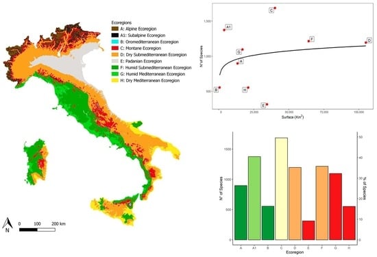
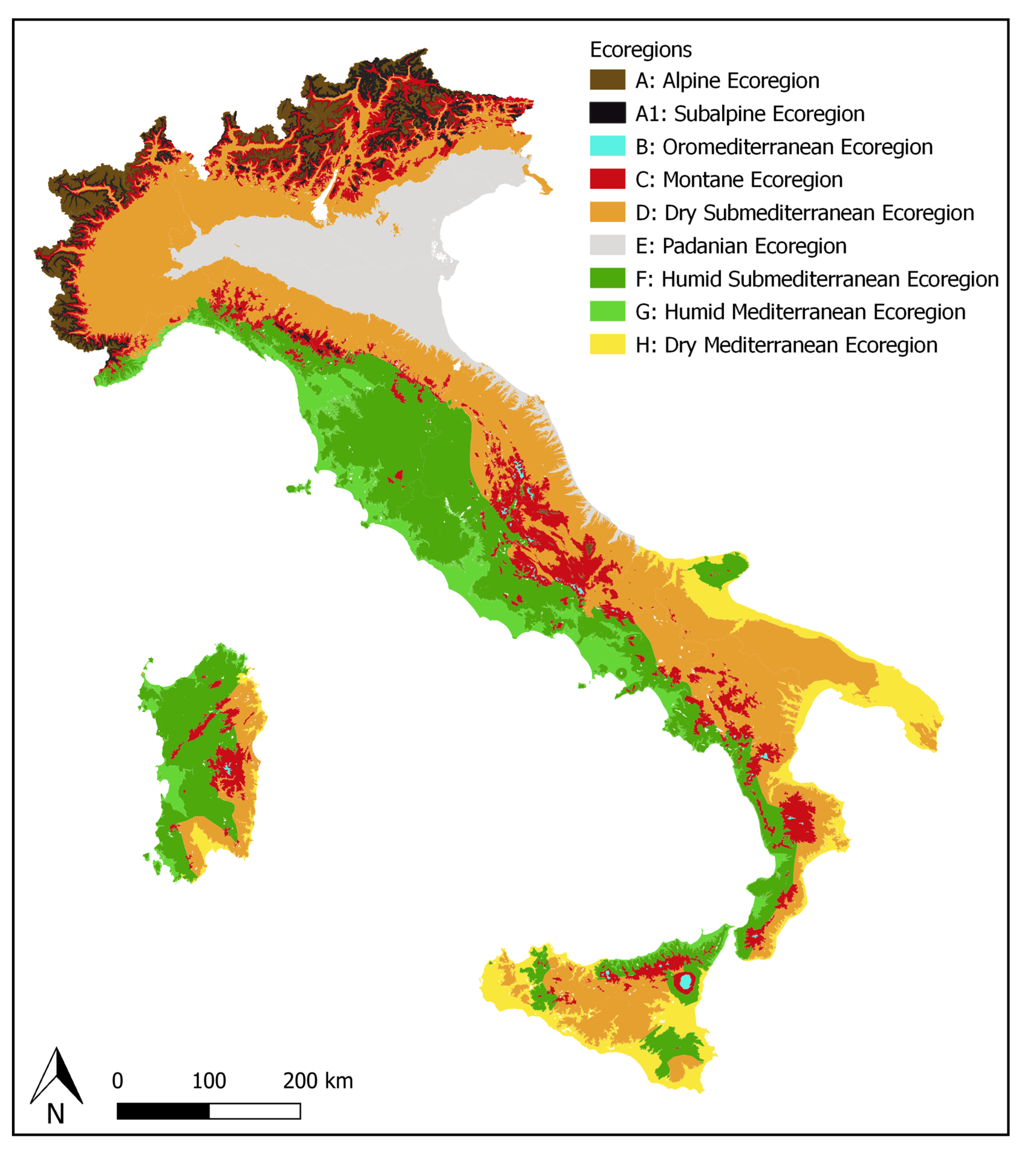
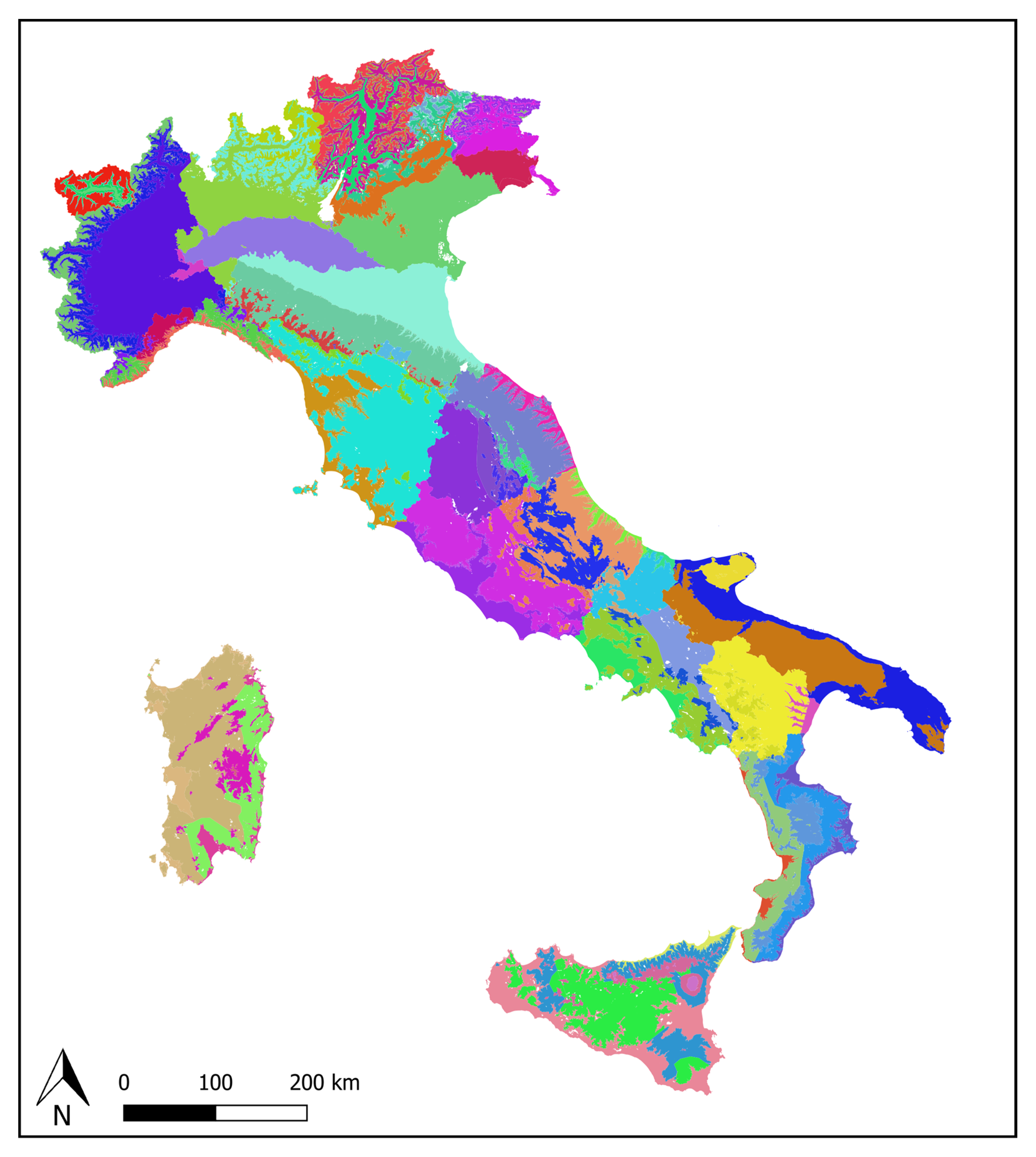
2.1. Ecoregions and OGUs

The distribution of lichen taxa is reported as presence/absence in the administrative regions [5]. A commonness-rarity score [4], ranging from “extremely rare” to “extremely common”, has been calculated for each infrageneric taxon, for each of the 9 ecoregions of the country (Figure 1) as originally delimited by Nimis [3]. Each administrative region includes several OGUs, deriving from the overlap of administrative and ecoregion borders. The delimitation of the 9 ecoregions mainly follows the altitudinal limits of the potential vegetation types, which can be very different from northern to southern, and from eastern to western Italy, so that altitude delimiting each ecoregion can differ among administrative regions (

Table 1. Altitudinal range for each of the 97 OGUs. For each OGU, its name in the database, the ecoregion to which it belongs (see Figure 1, and the text for details), and the elevation range are provided.

OGU	Administrative Region	Ecoregion	Altitudinal Range
1	Abruzzo	E	0–100
2	Abruzzo	D	101–900
3	Abruzzo	A	2001–4000
4	Abruzzo	C	901–2000
5	Basilicata	H	0–100
6	Basilicata	G	0–100
7	Basilicata	D	101–900
8	Basilicata	F	101–900
9	Basilicata	B	1701–4000
10	Basilicata	C	901–1700
11	Calabria	H	0–100
12	Calabria	G	0–100
13	Calabria	D	101–900
14	Calabria	F	101–900
15	Calabria	B	1701–4000
16	Calabria	C	901–1700
17	Campania	G	0–100
18	Campania	D	101–900
19	Campania	F	101–900
20	Campania	B	1701–4000
21	Campania	C	901–1700
22	Emilia Romagna	E	0–100
23	Emilia Romagna	D	101–900
24	Emilia Romagna	A1	1701–1900
25	Emilia Romagna	A	1901–4000
26	Emilia Romagna	C	901–1700
27	Friuli Venezia Giulia	E	0–100
28	Friuli Venezia Giulia	D	101–900
29	Friuli Venezia Giulia	A1	1701–1900
30	Friuli Venezia Giulia	A	1901–4000
31	Friuli Venezia Giulia	C	901–1700
32	Lazio	G	0–100
33	Lazio	B	1701–4000
34	Lazio	F	101–900
35	Lazio	C	901–1700
36	Liguria	G	0–250
37	Liguria	A1	1701–1900
38	Liguria	A	1901–4000
39	Liguria	D	251–900
40	Liguria	F	251–900
41	Liguria	C	901–1700
42	Lombardia	E	0–100
43	Lombardia	D	101–900
44	Lombardia	A1	1701–1900
45	Lombardia	A	1901–4000
46	Lombardia	C	901–1700
47	Marche	E	0–100
48	Marche	D	101–900
49	Marche	B	1701–4000
50	Marche	C	901–1700
51	Molise	H	0–100
52	Molise	D	101–900
53	Molise	B	1701–4000
54	Molise	C	901–1700
55	Piemonte	E	0–100
56	Piemonte	D	101–900
57	Piemonte	A1	1701–1900
58	Piemonte	A	1901–4000
59	Piemonte	C	901–1700
60	Puglia	H	0–100
61	Puglia	D	101–900
62	Puglia	F	101–900
63	Puglia	C	901–1700
64	Sardegna	H	0–50
65	Sardegna	G	0–50
66	Sardegna	B	1401–4000
67	Sardegna	D	51–700
68	Sardegna	F	51–700
69	Sardegna	C	701–1400
70	Sicilia	H	0–250
71	Sicilia	G	0–250
72	Sicilia	B	1601–4000
73	Sicilia	F	251–900
74	Sicilia	D	251–900
75	Sicilia	C	901–1600
76	Toscana	G	0–100
77	Toscana	D	101–900
78	Toscana	F	101–900
79	Toscana	A	1701–4000
80	Toscana	C	901–1700
81	Trentino Alto Adige	D	101–900
82	Trentino Alto Adige	A1	1701–1900
83	Trentino Alto Adige	A	1901–4000
84	Trentino Alto Adige	C	901–1700
85	Umbria	D	101–900
86	Umbria	F	101–900
87	Umbria	B	1701–4000
88	Umbria	C	901–1700
89	Val d’Aosta	D	101–900
90	Val d’Aosta	A1	1701–1900
91	Val d’Aosta	A	1901–4000
92	Val d’Aosta	C	901–1700
93	Veneto	E	0–100
94	Veneto	D	101–900
95	Veneto	A1	1701–1900
96	Veneto	A	1901–4000
97	Veneto	C	901–1700

).

A GIS map was generated from the digital elevation model (DEM) of the country, obtained by the national geoportal (http://www.pcn.minambiente.it), with a resolution of 20 m. The original map was split into administrative regions, and inside each region the ecoregions were delimited by means of the r.reclass, r.to.vect, and v.patch of the software GRASS GIS 7.4 (https://grass.osgeo.org/), thus producing a GIS map of a total of 97 OGUs (Figure 2). Subsequently, the ecoregions present in each region were extracted from each of the 20 raster maps using the assigned ranges of elevation (Table 1) using the function GRASS GIS r.reclass. The ecoregions occurring each administrative region were transformed into vectors (r.to.vect of GRASS GIS) and joined into a single map of all Italy (v.patch of GRASS GIS). The subdivision between “humid” and “dry” ecoregions is based on Nimis and Tretiach [2], in which the concept of “Thyrrenian Italy” and the influence of humid western winds to lichen communities were discussed. The “Padanian” ecoregion is a sub-Mediterranean portion of the country, including especially the whole Po plain, where high anthropization strongly affects lichen diversity [4]. Each of the 97 OGUs is made of a number of polygons ranging from 1 to n. Since computation complexity increases with the number of polygons, it was decided to take into account only the 20 larger polygons for each OGU. This allowed to drastically reduce computation complexity while retaining almost the whole surface of each OGU. In fact, discarding the smaller polygons led to the loss of 0.6% only of the total surface of the country. The number of ecoregions for each administrative region, together with their surface in percentage, are reported in

Table 2. Number of ecoregions for each Administrative region in Italy, and percentages of their surface areas in each region. The ecoregions are: Alpine (A), Subalpine (A1), Oromediterranean (B), Montane (C), Dry Submediterranean (D), Padanian (E), Humid Submediterranean (F), Humid Mediterranean (G), Dry Mediterranean (H).

Administrative Region	% A	% A1	% B	% C	% D	% E	% F	% G	% H	% Italy Surface	n° of Species	% of Species
Piemonte	12.6	3.64		16.65	65.22	1.85				1.48	1293	46.51
Valle D’Aosta	63.5	8.44		20.97	6.85	0				8.55	945	33.99
Lombardia	10.38	2.68		12.75	40.7	32.46				7.61	1295	46.58
Veneto	3.87	2.55		13.97	20.87	57.89				7.98	1175	42.27
Trentino A.A.	33.66	10.04		38.06	17.3					5.04	1579	56.8
Liguria	0.07	0.25		14.18	22.09		38.58	23.96		7.43	1089	39.17
Friuli V.G.	1.6	2.33		22.56	39.91	32.8				1.79	1049	37.73
Emilia-Romagna	0.02	0.14		7.81	42.68	49.18				4.51	775	27.88
Toscana	0.21			6.22	2.82		68.35	21.63		4.52	1205	43.35
Umbria			0.16	9.51	21.58		67.85			3.34	562	20.22
Marche			0.69	8.02	74.79	16.15				2.8	673	24.21
Molise			0.32	13.8	78.7				7.03	3.11	520	18.71
Lazio			0.87	10.71			62.47	25.27		2.6	878	31.58
Abruzzo	1.8			38.69	52.41	7.39				8.41	705	25.36
Puglia				0.3	50.36		7		42.28	5.7	629	22.63
Campania			0.05	9.36	28.08		40.23	21.3		6.09	844	30.36
Calabria			0.37	20.34	32.59		28.65	4.66	13.13	7.9	975	35.07
Basilicata			0.25	16.64	71.74		3.67	0.05	7.2	1.08	639	22.99
Sicilia			0.75	7.25	33.96		21.68	2.79	31.53	6.47	1168	42.01
Sardegna			0.17	10.72	21.46		52.61	8.32	5.76	3.59	1252	45.04

.

2.2. Functional Traits and Ecological Requirements

Information on species functional traits and ecological requirements were retrieved from ITALIC (see [4] for further details).

(A) Functional traits:

Growth form (crustose, crustose endolithic, crustose placodioid, leprose, squamulose, foliose umbilicate, foliose broad-lobed, foliose narrow-lobed; fruticose, fruticose filamentous lichens; non-lichenized).

Photobiont (chlorococcoid green algae other than Trentepohlia; green algae belonging to Trentepohlia; filamentous cyanobacteria (e.g., Nostoc), or coccoid cyanobacteria (e.g., Gloeocapsa).

Reproductive strategy (mostly sexually; mostly asexual, by soredia or soredia-like structures; mostly asexual by isidia; mostly asexual, by thallus fragmentation)

(B) Ecological requirements

Substrata (epiphytic on bark or wood; foliicolous on evergreen leaves; saxicolous; terricolous)

pH of the substratum (indicator values ranging from 1, very acid, to 5, strongly basic)

Eutrophication (indicator values ranging from 1, no eutrophication, to 5, high eutrophication)

Light (indicator values ranging from 1, very low solar radiation, to 5, very high solar radiation)

Aridity (indicator values ranging from 1, very humid conditions, to 5, very dry conditions)

2.3. Environmental Data

All environmental data were retrieved from freely accessible online sources (see details below).

Italy has a surface of about 300,000 square km, of which 35% is made of mountains, 42% of hills, and 23% of plains. Given the wide altitudinal and longitudinal gradients, the country hosts a wide array of climatic conditions.

Landscape analyses are based upon the vectorial maps of Corine Land Cover, IV level, 2012 (https://land.copernicus.eu/pan-european/corine-land-cover).

Landscape data were extracted for each OGU by using software v.overlay of GRASS GIS, within the environment Rstudio (4.0.2), and are:

Forest coverage: percentage of woodland cover (code 3.1)

Natural and semi-natural landscapes: percentage of surface occupied by patches of woodlands and semi-natural environments (code 3)

Urbanized areas: percentage of surface occupied by patches of artificial environments (code 1)

Diversity of the landscape: number of different Corinne IV level environments.

Geological data were extracted from the Carta Geologica d’Italia, obtained by the National Geoportal (http://www.pcn.minambiente.it). Since this map has a low resolution at a 1:500,000 scale (http://www.isprambiente.gov.it/it/cartografia) we have produced a simplified map, relevant to lichen ecology, by partitioning areas with a prevalence of siliceous or carbonatic rocks. For each OGU, the percentages of both types of substrata were extracted.

Topographic data were extracted from the national DEM (http://www.pcn.minambiente.it) by means of the Zonal statistics function of QGIS. The data are:

Minimum and maximum elevation.

Elevation diversity, expressed as the standard deviation of the elevation in an OGU.

Latitude of the centroid (WGS84), taken from the wider polygon of each OGU.

As far as pollutants are concerned, two deposition maps were used, both obtained from EMEP (European Monitoring and Evaluation Programme, http://www.emep.int/mscw/), which were used as proxies of eutrophication. Their resolution is 10 square kilometers.

Deposition maps:

Depositions of nitrogen oxides (NOx), expressed as mg/m², and

Depositions of ammonia (NH₃), and ammonium (NH₄⁺), expressed as mg/m².

Climate variables, depicted in raster files of 1 square kilometer of resolution:

Average yearly precipitation, expressed as mm/y, obtained from CHELSA CLIMATE (http://chelsa-climate.org)

Average mean temperature, expressed in °C, obtained from WORLDCLIM (http://www.worldclim.org/bioclim)

Temperature Seasonality, obtained from WORLDCLIM (http://www.worldclim.org/bioclim)

2.4. Data Analysis

The ecological and lichenological features of the 9 ecoregions were descriptively analyzed. For each variable, box plot charts were produced, in order to describe trends in environmental, climatic, and landscape variables. Once it was verified that the values of variables were assuming a non-normal distribution (Shapiro-Wilk test), the Kruskal–Wallis test [11] was applied to test differences. When a p-value < 0.05 was obtained, the Wilcoxon test was applied to each of the possible pairs [12]) to check for differences between ecoregions.

Species-area relationships across the 9 ecoregions were explored by means of Arrhenhius power function [13]: S = c∙Az

Where S is the number of taxa, A the area, and c and z two fitted parameters. The former represents the number of taxa expected per area unit, the latter is the angular coefficient of the straight line in a log-log space. The model was produced using the function “SSArrhenius” from the vegan package [14], The graph was produced by means of the ggplot2 package [15]. All analyses were conducted in R version 4.0.2 [16].

3. Results

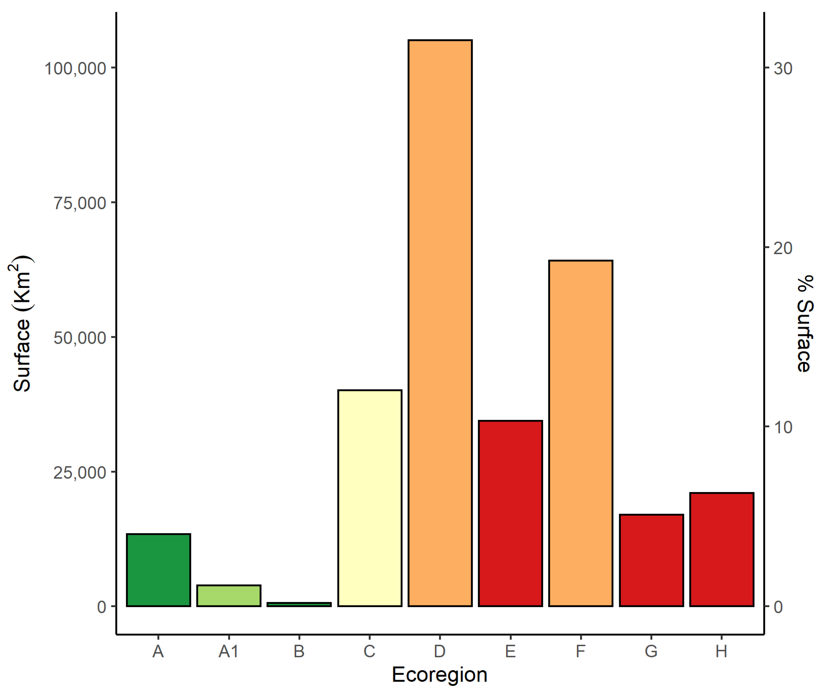
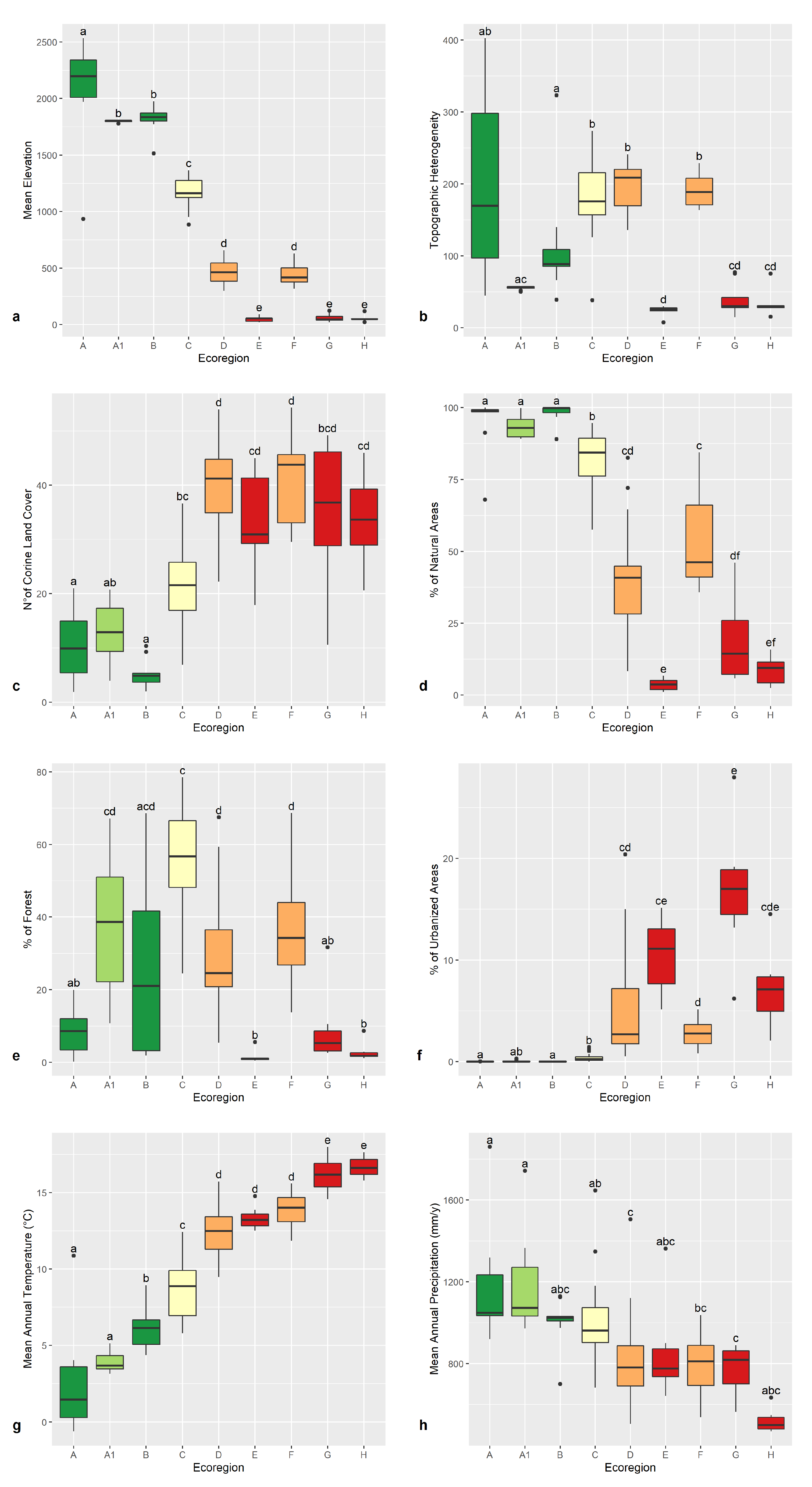
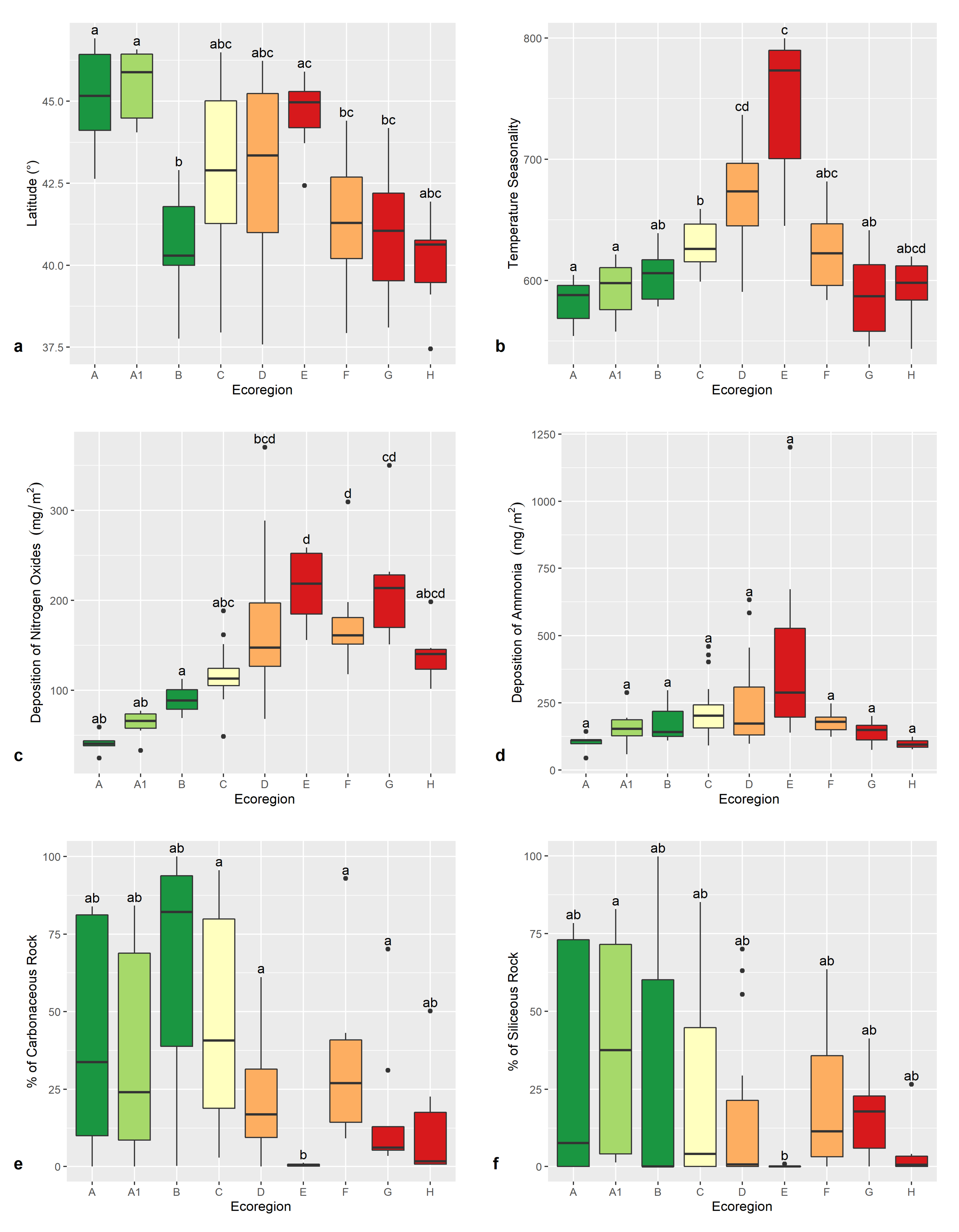
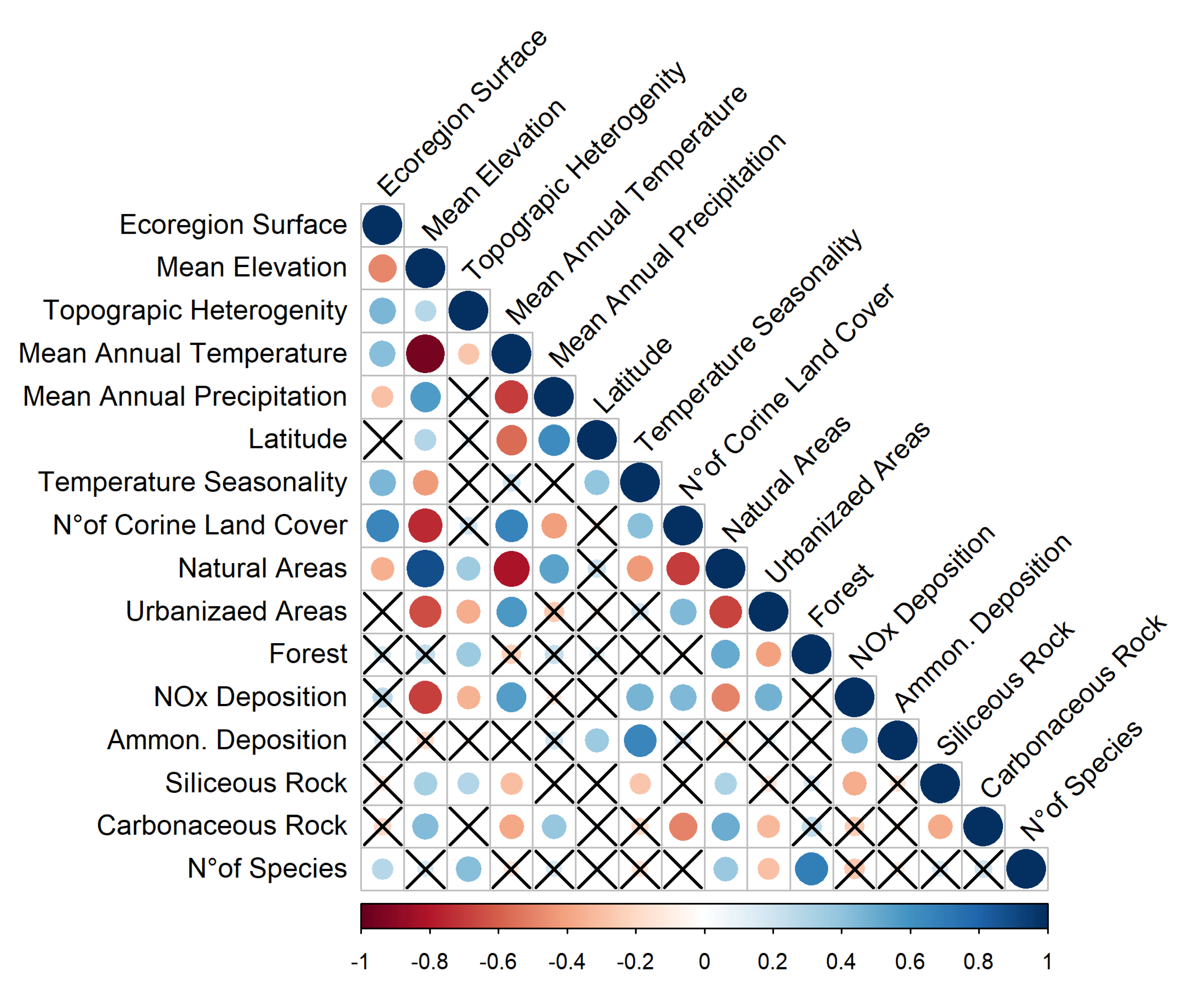
3.1. Environmental Features of the Ecoregions

The Dry Submediterranean (D) is the widest ecoregion (Figure 3). Together with the Humid Submediterranean (F), it covers ca. 60% of the country. The other low altitude ecoregions—Padanian (E), Dry (G), and Humid Mediterranean (H)—together occupy ca. 12% of the country. The Montane ecoregion (C), occupying ca. 13% of the country, is the only one occurring in all administrative regions. The Alpine (A), Subalpine (A1), and Oromediterranean (B) ecoregions have a very small surface area (ca. 10% of the country altogether).

Some ecoregions occupy the same altitudinal range, but in different parts of the country (Figure 4a). The Humid and Dry Mediterranean, the Humid and Dry Submediterranean, as well as the Padanian ecoregions are different geographical portions of a similar altitudinal range. The same applies for the Alpine-Subalpine and Oromediterranean ecoregions, which have very different biogeographic features, although occupying a similar altitudinal range. The Alpine ecoregion, while having a small surface, has a high topographic heterogeneity (Figure 4b), since it ranges from 2000 to 4000 m. However, the most heterogeneous are the Montane and Submediterranean ecoregions, since they span a wider latitudinal gradient.

Landscape diversity (Figure 4c) is higher in lowland ecoregions and decreases with altitude, while the contrary applies to the coverage of natural and semi-natural habitats (Figure 4d), which has a minimum in the Padanian ecoregion. At high altitudes, the surface occupied by natural and semi-natural habitats is always higher than 85%, while in the lowlands it is always lower than 20%.

Woodland coverage is higher in the Montane (60%), and Subalpine (40%) ecoregions (Figure 4e), while the higher percentages of disturbed areas (Figure 4f), are in the Padanian and the Humid and Dry Mediterranean ecoregions. The Oromediterranean ecoregion has the highest geographic variability in the percent of woodland cover, being scattered in several administrative regions, and on different mountain peaks.

Average temperature (°C), and precipitation (mm), as expected, have an opposite trend from high to low altitudes OGUs (Figure 4g,h). Low-altitude ecoregions encompass a broader latitudinal span than high-altitude ecoregions (Figure 5a), the Alpine and Subalpine ecoregions being limited to the Alps and Central Apennines, while the Oromediterranean ecoregion is limited to the southernmost high mountains. The Padanian ecoregion is limited to the Po Plain, where temperature seasonality (Figure 5b) is higher, indicating a relevant climatic continentality.

As far as nitrogen oxides (NO_X) are concerned (Figure 5c), higher deposition prevails at lower altitudes, where anthropization is higher and agriculture is intensive. As far as ammonia is concerned (NH₄, NH₄⁺), no significant differences can be evidenced in the average deposition among OGUs in different ecoregions, even if, as expected, the heaviest depositions occur in the Padanian OGUs (Figure 5d). In the case of nitrogen pollutants, however, the coarse scale of the original data (10 × 10 km) could originate a bias in the analysis.

The distribution of the two main types of lithologic substrate—carbonatic and siliceous rocks, Figure 5e,f) did not differ among OGUs of different ecoregions. The average percentage of the surface of OGUs occupied by rocky substrata ranges from 0% to 95% in high-altitude ecoregions, being lower in low-altitude ecoregions, and close to zero in the Padanian ecoregion, where agriculture occupies practically the whole surface.

Variables describing the environmental conditions of the 97 OGUs are often correlated between each other (Figure 6).

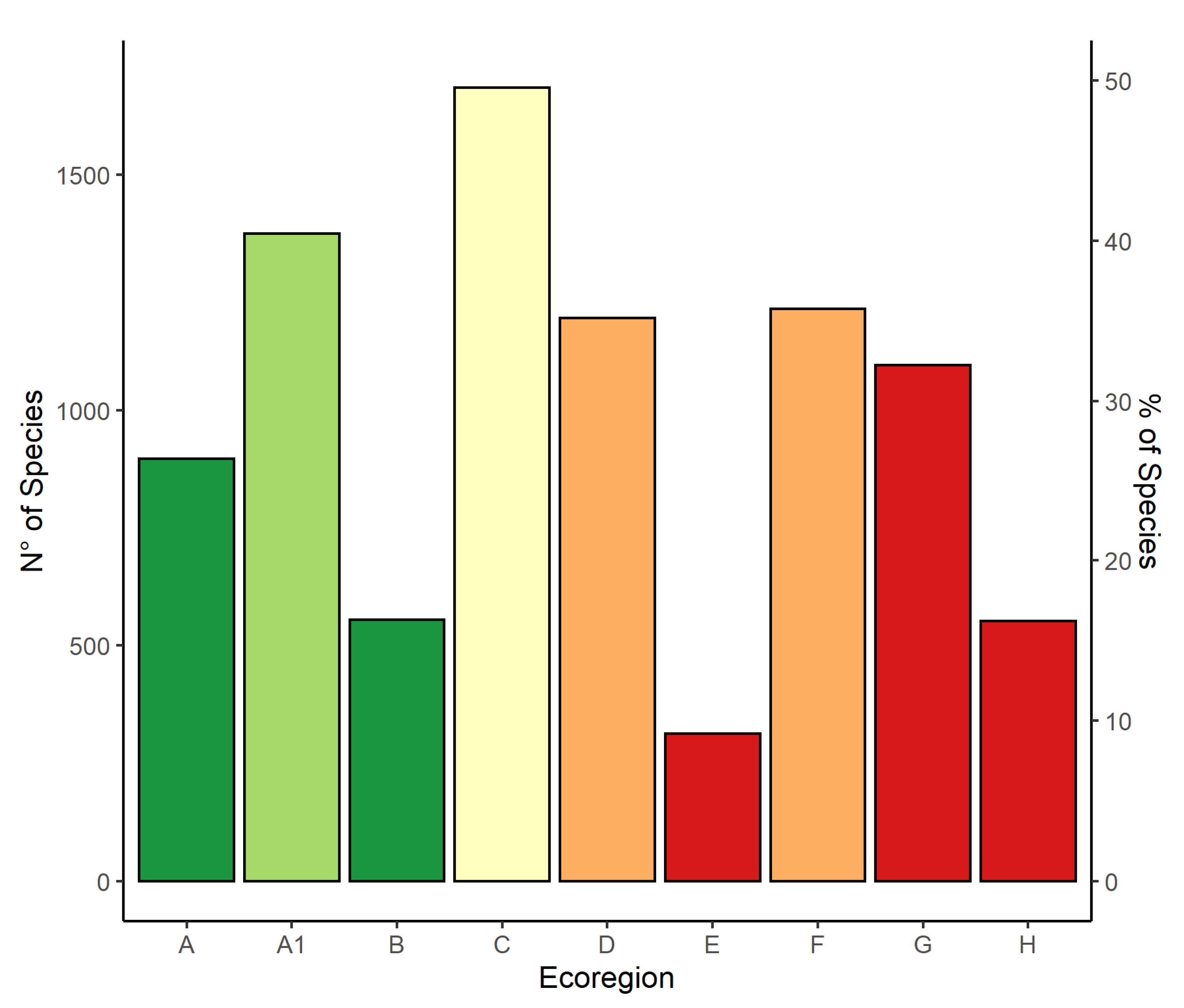
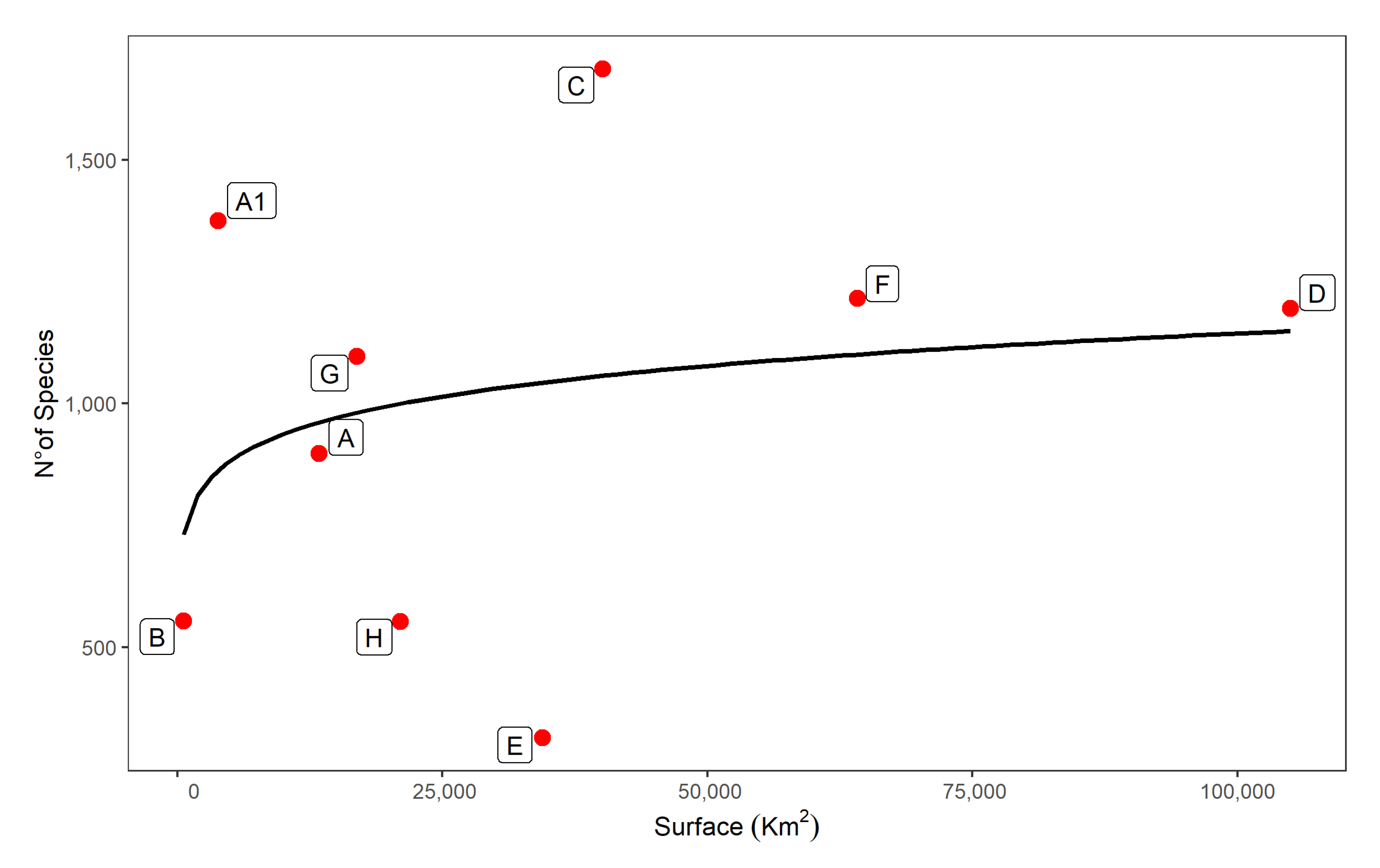
3.2. Lichen Richness in the Ecoregions

Species richness is positively correlated to total surface, topographic heterogeneity, coverage of natural and semi-natural habitats, and of woodlands, and is negatively correlated to the amount of urbanized, heavily disturbed areas (Figure 6). Thus, the Montane ecoregion has the highest species richness, the Padanian ecoregion the lowest (Figure 7).

The ecoregions with the highest woodland coverage (Montane and Subalpine, Figure 4e), are also those with the highest species richness, hosting more than 50% of all taxa known to occur in the country. These two ecoregions, however, strongly differ in surface (Figure 3), as well as in latitudinal range (Figure 5a). The Subalpine ecoregion is restricted to the northern part of the country and has a very small surface (less than 2%), while the Montane ecoregion occurs in all administrative regions, and has a wider surface (ca. 13%). The Dry and Humid Submediterranean, Alpine, and Humid Mediterranean ecoregions host between 35% and 50% of the taxa known to occur in Italy. On the contrary, heavily disturbed areas have the lowest lichen diversity (Padanian and Dry Mediterranean ecoregions, Figure 4f), with less than 500 taxa each. The Oromediterranean ecoregion as well has a low number of taxa, but it occupies a very small surface, less than 0.5% of the country (Table 2). The OGUs in the Humid Mediterranean ecoregion, while heavily anthropized, host a relatively high lichen diversity, comparable to that of the two Submediterranean ecoregions. Average latitude (Figure 5a) of the OGUs of the 9 ecoregions does not reflect species richness (Figure 7).

The relationship between number of taxa and surface of ecoregions is reported in Figure 8. Species richness in 5 out of 9 ecoregions (Oromediterranean, Alpine, Humid and Dry submediterranean, and Humid Mediterranean) is well described by the model (significance level of the model: alpha = 0.05). Two ecoregions (Subalpine, Montane) have a larger number of taxa than expected, while two (Padanian and Dry Mediterranean) host far fewer taxa than expected.

Table 3. Incidence (absolute numbers and percentages) of taxa with oceanic, suboceanic, and subcontinental phytoclimatic range in the lichen flora of the 9 ecoregions.

	Oceanic	Suboceanic	Subcontinental
Alpine	0	23 (2.6%)	26 (2.9%)
Subalpine	1 (0.1%)	69 (5.0%)	46 (3.4%)
Oromediterranean	0	15 (2.7%)	21 (3.8%)
Montane	19 (1.1%)	262 (15.5%)	72 (4.3%)
Humid Submediterranean	22 (1.8%)	317 (26.0%)	49 (3.3%)
Dry Submediterranean	9 (0.7%)	239 (19.9%)	65 (5.4%)
Humid Mediterranean	40 (3.6%)	313 (28.4%)	33 (3.0%)
Dry Mediterranean	0	58 (10.4%)	37 (6.6%)
Padane	0	22 (7.0%)	4 (1.3%)

Reports the incidence of taxa with oceanic, suboceanic, and subcontinental distribution patterns in the ecoregions. At lower elevations (Mediterranean and Submediterranean ecoregions), the basic difference between the western and eastern sides of the Italian Peninsula is confirmed, with a higher incidence of oceanic-suboceanic species with subtropical affinities along the western side, which is subject to the influence of humid, maritime air masses. On the contrary, very low values are reached in the Alpine Subalpine, Oromediterranean, and Dry Mediterranean ecoregions. Subcontinental species have the highest incidence in the Dry Mediterranean ecoregion, mainly due to the occurrence of steppic or desert species.

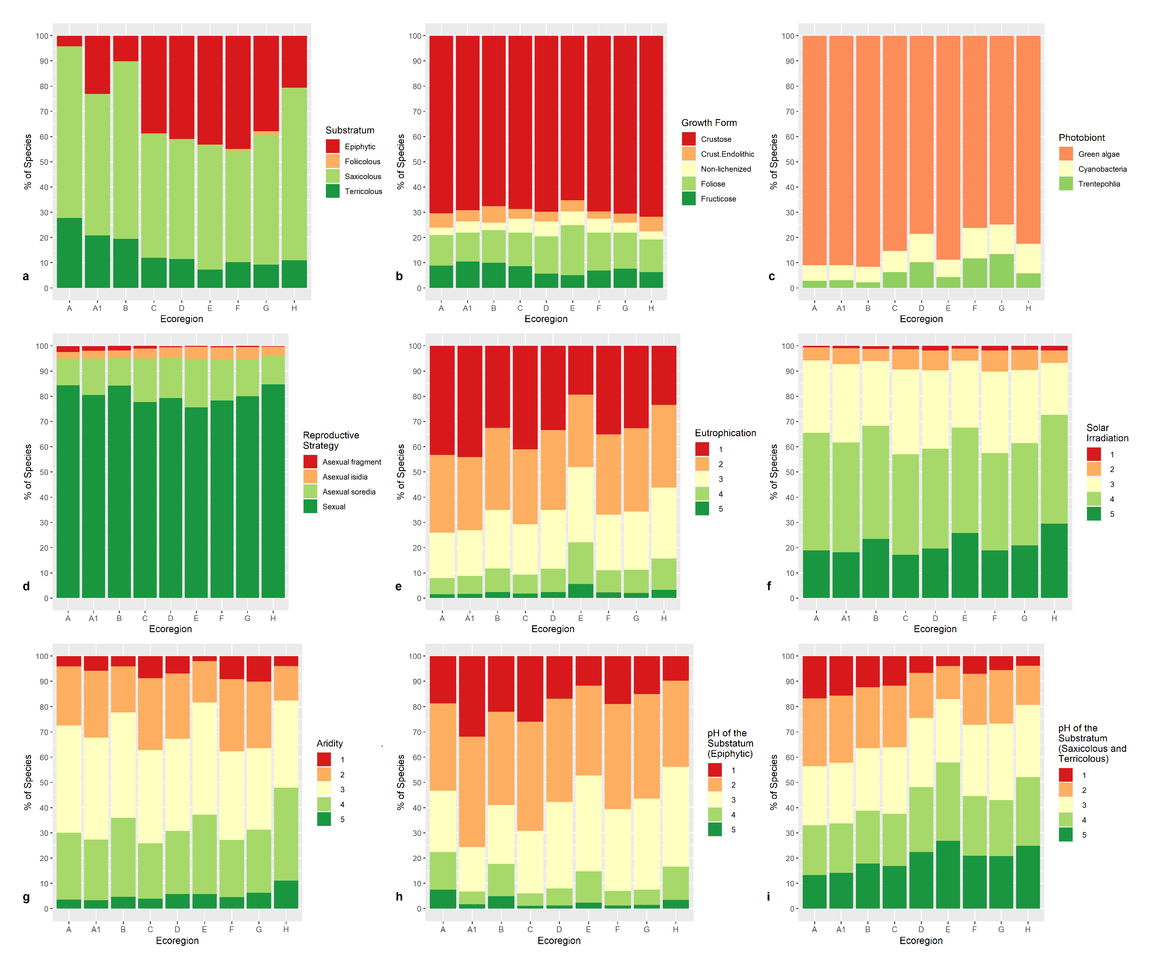
3.3. Lichen Traits and Ecological Requirements in the Ecoregions

As far as substrates are concerned (Figure 9a), epiphytic taxa are obviously scarce in the high-altitude northern ecoregions (Alpine and Subalpine), saxicolous and terricolous species being the most abundant, the latter reaching their maximum, up to 20% of the total, due to the presence of Alpine tundras. Saxicolous taxa have the maximum in the Dry Mediterranean ecoregion, which has a scanty woodland cover. Epiphytes have the maximum (almost 50%) in the Montane, the Submediterranean, and the Humid Mediterranean ecoregions. Epiphyllous taxa are a very minor component of the Italian lichen flora (30 taxa), which occur almost exclusively in the Humid Mediterranean ecoregion, which is well in accordance with their mainly tropical affinities. Except for the type of photobiont, species traits do not show distinctive patterns across ecoregions. Crustose taxa are 65–70% of the whole lichen biota (Figure 9b). Endolithic taxa, however, occur mostly in ecoregions with a small coverage of woodlands (Alpine, Dry Mediterranean, Oromediterranean). Taxa with chlorococcoid photobionts are the most numerous in all ecoregions (Figure 9c). They have the minimum in the Submediterranean and Humid Mediterranean ecoregions, where taxa with Trentepholia have their maximum (10–12%). Species with cyanobacteria have their maximum in the same ecoregions, plus the Dry Mediterranean ecoregion, where they reach ca. 12% of the total, with the highest incidence of coccoid cyanobacteria typical of desert habitats. The sexual reproductive strategy (Figure 9d) is the most represented, ranging from 78% to 85% in each ecoregion. Reproduction by thallus fragmentation is most frequent in high-altitude ecoregions (Alpine, Subalpine, and Oromediterranean).

Taxa which are adapted to high eutrophication (values 4 and 5 of the index) are ca. 20% of the total lichen biota only in the Padanian ecoregion (Figure 9e), where anthropization is the highest. Species related to weakly disturbed habitats (indicator value 1) are most abundant in the Alpine, Oromediterranean and Montane ecoregions. Light indicator values have no distinctive pattern across ecoregions (Figure 9f) even if there is a relatively higher abundance of taxa adapted to shaded habitats (values 1 and 2 of the light index) in the ecoregions which are richer in woodlands (Montane, Dry and Humid Submediterranean). Taxa which are adapted to humid conditions (values 1 and 2 of the aridity index, Figure 9g) are also most abundant in the Montane, Submediterranean, and Humid Mediterranean ecoregions. Substrate acidity is depicted separately for epiphytic, saxicolous, and terricolous lichens (Figure 9h). Species adapted to more acidic substrata (values 1 and 2 of the index) are most abundant in those ecoregions where conifers and beech dominate (Subalpine, and Montane). Saxicolous and terricolous taxa maximize their richness in upland areas with acidic substrata (Figure 9i).

4. Discussion

Our GIS-based analysis allowed us to describe, for the first time, the main features of the 9 ecoregions adopted in ITALIC, highlighting the main differences that could explain the main patterns of lichen richness, functional traits, and ecological requirements. While the 9 ecoregions are bioclimatically well-delimited, they are also part of a continuum, and often share similar features, which gradually change with altitude and latitude. The ecological factors used for delimiting the ecoregions are those which are known to considerably influence lichen species richness and diversity, shaping the lichen biota of the country.

The areas of the OGUs belonging to each ecoregion are strongly affected by altitude, with generally smaller OGUs at higher elevations. Theoretical models of species-area relationship (SAR) evidence that the increase in area is often correlated with an increase in habitat heterogeneity, thus leading to higher richness [17,18,19,20]. However, in Italy, the area occupied by natural and semi-natural habitats strongly increases with altitude, which positively affects lichen richness. Thus, the combined effect of reduced area and increase of “naturality” weakens the positive correlation between area and species richness. In particular, the Subalpine ecoregion, restricted to the northern regions, and with a small surface, has a high species richness, comparable to that of the much broader Montane ecoregion. In particular, larch and stone-pine forests of the Subalpine ecoregion were found to be a hotspot of lichen diversity of particular conservation concern [21,22,23]. As far as the Montane ecoregion is concerned, the high species richness is probably related to its wide latitudinal extent, since it ranges throughout the country, spanning a relevant biogeographic gradient [24,25]. This should be reflected in heterogeneous community composition across sites [1], a pattern which would, however, require further investigation.

In the Padanian and Dry Mediterranean ecoregions, species richness is negatively impacted by high anthropization [26], even where the landscape is heterogeneous. The Padanian ecoregion is the most disturbed, virtually lacking natural or semi-natural habitats that were replaced by intensive agriculture, industrial areas, and urban areas. Under these circumstances, depositions of both nitrogen oxides and ammonia, as well as habitat destruction and fragmentation directly impact on species richness [27,28]. The interplay between these drivers caused the historical depauperation of a previously rich and specialized lichen biota that was replaced by a few generalist species which are homogenizing the lichen communities [29,30].

Species richness is also associated with topographic heterogeneity, likely due to its effect on micro- and meso-climatic conditions. This is particularly evident in the high species richness of the Alpine, Subalpine, and Oromediterranean ecoregions, even if they account for a very small surface (ca 6.5%). This pattern is consistent with the outstanding richness of the lichen biota of the Alps [5]. However, besides environmental factors, this situation may also reflect an exploration bias, since high-elevation areas have a long-lasting tradition of lichenological surveys.

Our analysis also revealed some robust patterns of species functional traits and ecological features across the 9 ecoregions. For example, lichens with Trentepohlia photobionts have their maximum in Submediterranean and Humid Mediterranean ecoregions, which is in accordance with their affinity for warm-humid conditions [31,32,33]. At low temperatures, these taxa are less competitive than other lichens [34], since trentepohlioid algae are more prone to freezing [35]. While a sexual reproductive strategy prevails in all ecoregions, thallus fragmentation, a particular type of asexual reproduction, seems to be clearly linked to high altitudes, as already observed by [36]. This may reflect an adaptation to cold conditions [37], and to the presence of lichen-grazing mammals in arctic-subarctic ecosystems dominated by tundras with many species of Cladonia, in which this strategy is often adopted.

Substrate availability is a major driver of lichen distribution in the different ecoregions. Epiphytic lichens are scarce or absent in the Alpine ad Oromediterranean ecoregions, which by definition are devoid of trees. Terricolous species are most abundant in sites where agriculture and urbanization are limited, or absent. Saxicolous species are most abundant in ecoregions with low coverage of woodlands, as the Alpine, Oromediterranean, and Dry Mediterraneans. This does not apply to the Padanian ecoregion, where the prevalence of sedimentary substrates, heavy anthropization, and intensive agricultural practices reduce the availability of saxicolous habitats.

Substrate pH is another relevant factor which contributes to lichen species richness [38]. Epiphytic species growing on acidic bark prevail in the communities of the Subalpine and Montane ecoregions, where the incidence of coniferous forests (Corine Land Cover code 3.2.2) is higher. The Subalpine ecoregion is characterized by woods dominated by Larix decidua and Picea abies, while Abies alba and Fagus sylvatica, whose bark is acidic as well, are characteristic of the Montane ecoregion [39]. Acidophilic saxicolous and terricolous lichens reach a maximum at high altitudes.

Nimis and Schiavon [40] in a study of epiphytic lichen vegetation along the western coast of peninsular Italy, showed that this is basically different from that of the eastern coast. The western side of the Italian Peninsula has a mild-humid climate under the influence of Tyrrhenian maritime winds, while the eastern, Adriatic side, located on the lee-side of the Apennines, is subject to cold-dry air masses from the Balkans during winter. This basic bioclimatic difference results in important compositional differences between the humid and dry Mediterranean/Submediterranean ecoregions, the former hosting a much higher number of species with oceanic/suboceanic distribution patterns and tropical/subtropical affinities.

Overall, the exploration of the Italian lichen biota is still a work in progress [3]. Some regions are still underexplored, especially in the South, new taxa being reported every year (e.g., [41]). Our research could provide a baseline for further advancements in the understanding of species richness and community composition of Italian lichens at a regional scale.

References

1. Nascimbene, J.; Benesperi, R.; Brunialti, G.; Catalano, I.; Dalle Vedove, M.; Grillo, M.; Isocrono, D.; Matteucci, E.; Potenza, G.; Puntillo, D.; et al. Patterns and drivers of β-diversity and similarity of Lobaria pulmonaria communities in Italian forests. J. Ecol. 2013, 101, 493–505. [Google Scholar] [CrossRef] [Green Version]
2. Nimis, P.L.; Tretiach, M. Delimiting Tyrrhenian Italy. A lichen foray in the SW part of the Peninsula. Bibl. Lichenol. 2004, 88, 465–478. [Google Scholar]
3. Nimis, P.L. The Lichens of Italy: An Annotated Catalogue; Monografie XII; Museo Regionale Scienze Naturali di Torino: Torino, Italy, 1993; p. 897. [Google Scholar]
4. Nimis, P.L.; Martellos, S. ITALIC, a database on Italian Lichens. Bibl. Lichenol. 2002, 82, 271–282. [Google Scholar]
5. Nimis, P.L.; Hafellner, J.; Roux, C.; Clerc, P.; Mayrhofer, H.; Martellos, S.; Bilovitz, P.O. The lichens of the Alps—An annotated checklist. MycoKeys 2018, 31, 1–634. [Google Scholar] [CrossRef] [Green Version]
6. Martellos, S. From a textual checklist to an information system: The case study of ITALIC, the Information System on Italian Lichens. Plant. Biosyst. 2012, 146, 764–770. [Google Scholar] [CrossRef]
7. Nimis, P.L. The Lichens of Italy: A Second Annotated Catalogue; EUT: Trieste, Italy, 2016; p. 739. [Google Scholar]
8. Nimis, P.L.; Martellos, S.; Chiarucci, A.; Ongaro, S.; Peplis, M.; Pittao, E.; Nascimbene, J. Exploring the relationships between ecology and species traits in cyanolichens: A case study in Italy. Fungal Ecol. 2020, 47, 100950. [Google Scholar] [CrossRef]
9. Jørgensens, P.M. Distribution Patterns of Lichens in the Pacific Region. Aust. J. Bot. Suppl. Ser. 1983, 13, 43–66. [Google Scholar]
10. Rubio-Salcedo, M.; Psomas, A.; Prieto, M.; Zimmermann, N.E.; Martìnez, I. Case study of the implications of climate change for lichen diversity and distributions. Biodivers. Conserv. 2017, 26, 1121–1141. [Google Scholar] [CrossRef]
11. Kruskal, W.H.; Wallis, W.A. Use of Ranks in One-Criterion Variance Analysis. J. Am. Stat. Assoc. 1952, 47, 583–621. [Google Scholar] [CrossRef]
12. Fotopoulos, S. Introduction to Modern Nonparametric Statistics. Technometrics 2004, 46, 488–489. [Google Scholar] [CrossRef]
13. Arrhenius, O. Species and area. J. Ecol. 1921, 9, 95–99. [Google Scholar] [CrossRef] [Green Version]
14. Oksanen, J.; Blanchet, F.G.; Kindt, R.; Legendre, P.; Minchin, P.; O’Hara, B.; Simpson, G.; Solymos, P.; Stevens, H.; Wagner, H. Vegan: Community Ecology Package. R Package Version 2.2-1, R Foundation for Statistical Computing: Vienna, Austria, 2015.
15. Wickham, H. ggplot2: Elegant Graphics for Data Analysis; Springer: New York, NY, USA, 2016. [Google Scholar]
16. R Core Team. R: A Language and Environment for Statistical Computing; R Foundation for Statistical Computing: Vienna, Austria, 2019. [Google Scholar]
17. Gleason, H.A. On the Relation between Species and Area. Ecology 1922, 3, 158–162. [Google Scholar] [CrossRef]
18. Lawrey, J. The Species-Area Curve as an Index of Disturbance in Saxicolous Lichen Communities. Bryologist 1991, 94, 377–382. [Google Scholar] [CrossRef]
19. Scheiner, S.; Chiarucci, A.; Fox, G.; Helmus, M.; McGlinn, D.; Willig, M. The underpinnings of the relationship of species richness with space and time. Ecol. Monogr. 2011, 81, 195–213. [Google Scholar] [CrossRef] [Green Version]
20. Wilson, B.; Chiarucci, A. Do plant communities exist? Evidence from scaling-up local species-area relations to the regional level. J. Veg. Sci. 2009, 11, 773–775. [Google Scholar]
21. Nascimbene, J.; Martellos, S.; Nimis, P.L. Epiphytic lichens of tree-line forests in the Central-Eastern Italian Alps and their importance for conservation. Lichenologist 2006, 38, 373–382. [Google Scholar] [CrossRef]
22. Nascimbene, J.; Marini, L.; Motta, R.; Nimis, P.L. Lichen diversity of coarse woody habitats in a Pinus-Larix stand in the Italian Alps. Lichenologist 2008, 40, 153–163. [Google Scholar] [CrossRef]
23. Nascimbene, J.; Thor, G.; Nimis, P.L. Habitat-types and lichen conservation in the Alps—Perspectives from a case study in the Stelvio National Park (Italy). Plant. Biosyst. 2012, 146, 428–442. [Google Scholar] [CrossRef]
24. Chiarucci, C.; Nascimbene, J.; Campetella, G.; Chelli, S.; Dainese, M.; Giorgini, D.; Landi, S.; Lelli, C.; Canullo, R. Exploring patterns of beta-diversity to test the consistency of biogeographical boundaries: A case study across forest plant communities of Italy. Ecol. Evol. 2019, 9, 11716–11723. [Google Scholar] [CrossRef]
25. Guttova, A.; Fackovcova, Z.; Martellos, S.; Paoli, L.; Munzi, S.; Pittao, E.; Ongaro, S. Ecological specialization of lichen congeners with a strong link to Mediterranean-type climate: A case study of the genus Solenopsora in the Apennine Peninsula. Lichenologist 2019, 51, 75–88. [Google Scholar] [CrossRef]
26. Cislaghi, C.; Nimis, P.L. Lichens, air pollution and lung cancer. Nature 1997, 387, 463–464. [Google Scholar] [CrossRef] [PubMed]
27. Giordani, P.; Calatayud, V.; Stofer, S.; Seidling, W.; Granke, O.; Fischer, R. Detecting the nitrogen critical loads on European forests by means of epiphytic lichens. A signal-to-noise evaluation. For. Ecol. Manag. 2014, 311, 29–40. [Google Scholar] [CrossRef]
28. Contardo, T.; Giordani, P.; Paoli, L.; Vannini, A.; Loppi, S. May lichen biomonitoring of air pollution be used for environmental justice assessment? A case study from an area of N Italy with a municipal solid waste incinerator. Environ. Forensics 2018, 19, 265–276. [Google Scholar] [CrossRef]
29. Nascimbene, J.; Marini, L. Oak forest exploitation and black locust invasion caused severe shifts in epiphytic lichen communities. Sci. Total Environ. 2010, 408, 5506–5512. [Google Scholar] [CrossRef]
30. Nascimbene, J.; Lazzaro, L.; Benesperi, R. Patterns of beta-diversity and similarity reveal biotic homogenization of epiphytic lichen communities associated with the spread of Black locust forests. Fungal. Ecol. 2015, 14, 1–7. [Google Scholar] [CrossRef]
31. van Herk, C.M.; Aptroot, A.; van Dobben, H.F. Long-term monitoring in the Netherlands suggests that lichens respond to global warming. Lichenologist 2002, 34, 141–154. [Google Scholar] [CrossRef] [Green Version]
32. Aptroot, A.; van Herk, C.M. Further evidence of the effects of global warming on lichens, particularly those with Trentepohlia phycobionts. Environ. Pollut. 2007, 146, 293–298. [Google Scholar] [CrossRef]
33. Marini, L.; Nascimbene, J.; Nimis, P.L. Large-scale patterns of epiphytic lichen species richness: Photobiont-dependent response to climate and forest structure. Sci. Total Environ. 2011, 409, 4381–4386. [Google Scholar] [CrossRef]
34. Nascimbene, J.; Marini, L. Epiphytic lichen diversity along elevational gradients: Biological traits reveal a complex response to water and energy. J. Biogeogr. 2015, 42, 1222–1232. [Google Scholar] [CrossRef]
35. Kappen, L. Plant activity under snow and ice, with particular reference to lichens. Arctic 1993, 46, 297–302. [Google Scholar] [CrossRef] [Green Version]
36. Jahns, H.M. Felci, Muschi, Licheni d’Europa; Franco Muzzio Editore: Padova, Italy, 1992. [Google Scholar]
37. Bässler, C.; Cadotte, M.W.; Beudert, B.; Heibl, C.; Blaschke, M.; Bradtka, J.H.; Langbehn, T.; Werth, S.; Müller, J. Contrasting patterns of lichen functional diversity and species richness across an elevation gradient. Ecography 2015, 38, 689–698. [Google Scholar] [CrossRef]
38. Nash, T.H. Lichen Biology; Cambridge University Press: Cambridge, UK, 2012. [Google Scholar]
39. Grodzińska, K. Acidity of tree bark as a bioindicator of forest pollution in Southern Poland. Water Air Soil Pollut 1977, 8, 3–7. [Google Scholar] [CrossRef]
40. Nimis, P.L.; Schiavon, L. The epiphytic lichen vegetation of the Tyrrhenian coasts in Central Italy. Ann. di Bot. 1986, 14, 39–67. [Google Scholar]
41. Ravera, S.; Puglisi, M.; Vizzini, A.; Totti, C.; Arosio, G.; Benesperi, R.; Bianchi, E.; Boccardo, F.; Briozzo, I.; Dagnino, D.; et al. Notulae to the Italian flora of algae, bryophytes, fungi and lichens: 8. Ital. Bot. 2019, 8, 47–62. [Google Scholar] [CrossRef]
Figure 1. The 9 ecoregions adopted in ITALIC: Alpine (A), Subalpine (A1), Oromediterranean (B), Montane (C), Dry Submediterranean (D), Padanian (E), Humid Submediterranean (F), Humid Mediterranean (G), Dry Mediterranean (H).
Diversity 12 00294 g001
Figure 2. The 97 OGUs in which Italy was divided by combining administrative and ecoregional subdivisions.
Diversity 12 00294 g002
Figure 3. Surface (in km2, and in percentage of total surface area), of the 9 ecoregions: Alpine (A), Subalpine (A1), Oromediterranean (B), Montane (C), Dry Submediterranean (D), Padanian (E), Humid Submediterranean (F), Humid Mediterranean (G), Dry Mediterranean (H). Similar colors of the bars depict ecoregions occupying the same altitudinal range. Color codes are green (high-altitude ecoregions), yellow (Montane ecoregion), orange (Submediterranean ecoregions), and red (Mediterranean ecoregions).
Diversity 12 00294 g003
Figure 4. Box-plot graphs depicting average altitude (m) (a), topographic diversity (b), landscape heterogeneity (c), percentage of natural and semi-natural habitats (d), percentage of woodland surface (e), percentage of anthropized surface (f), average mean temperature (g), average precipitation (h) for the OGUs of the 9 ecoregions: Alpine (A), Subalpine (A1), Oromediterranean (B), Montane (C), Dry Submediterranean (D), Padanian (E), Humid Submediterranean (F), Humid Mediterranean (G), Dry Mediterranean (H). Significant differences are labeled by different letters (Wilcoxon test). Box colors show ecoregions with the same altitudinal range. Color codes are green (high-altitude ecoregions), yellow (Montane ecoregion), orange (Submediterranean ecoregions), and red (Mediterranean ecoregions).
Diversity 12 00294 g004
Figure 5. Box-plot graphs depicting average latitude (a), average temperature seasonality (b), average deposition of nitrogen oxides (NOX) (mg/m2) (c), average deposition of ammonia (NH4, NH4+) (mg/m2) (d), percentage of carbonatic substrata (e), and percentage of siliceous substrata (f) for the OGUs of the 9 ecoregions: Alpine (A), Subalpine (A1), Oromediterranean (B), Montane (C), Dry Submediterranean (D), Padanian (E), Humid Submediterranean (F), Humid Mediterranean (G), Dry Mediterranean (H). Significant differences are labeled by different letters (Wilcoxon test). Box colors show ecoregions with the same altitudinal range. Color codes are green (high-altitude ecoregions), yellow (Montane ecoregion), orange (Submediterranean ecoregions), and red (Mediterranean ecoregions).
Diversity 12 00294 g005
Figure 6. Correlation matrix among variables. Negative correlations are in red, positive correlations in blue. Correlations with p value > 0.01 are highlighted with a X. Strength of correlation is expressed in a scale ranging from −1 (strongly negative) to 1 (strongly positive).
Diversity 12 00294 g006
Figure 7. Bar-plot graph depicting the abundance of taxa occurring in each of the 9 ecoregions: Alpine (A), Subalpine (A1), Oromediterranean (B), Montane (C), Dry Submediterranean (D), Padanian (E), Humid Submediterranean (F), Humid Mediterranean (G), Dry Mediterranean (H). Similar colors of the bars depict ecoregions occupying the same altitudinal range. Color codes are green (high-altitude ecoregions), yellow (Montane ecoregion), orange (Submediterranean ecoregions), and red (Mediterranean ecoregions).
Diversity 12 00294 g007
Figure 8. Relationship between number of taxa and total surface (SAR: species-area relationship) built by following the Arrhenius model (S = cAz). The surface is expressed in square km. Letters in capital are the 9 ecoregions: Alpine (A), Subalpine (A1), Oromediterranean (B), Montane (C), Dry Submediterranean (D), Padanian (E), Humid Submediterranean (F), Humid Mediterranean (G), Dry Mediterranean (H).
Diversity 12 00294 g008
Figure 9. Bar-plot graphs depicting the distribution of lichen taxa per substratum (a), growth form (b), photobiont (c), reproductive strategy (d), along with the values of the indicator of eutrophication (from 1—no eutrophication, to 5—very high eutrophication) (e), light (from 1—in very shaded situations, to 5—in sites with very high direct solar irradiation) (f), aridity (from 1—hygrophytic, to 5, very xerophytic) (g), and pH of the substratum (from 1—very acid substrata, to 5—basic substrata) for epiphytic (h), and terricolous and saxicolous taxa (i) in the OGUs of the 9 ecoregions: Alpine (A), Subalpine (A1), Oromediterranean (B), Montane (C), Dry Submediterranean (D), Padanian (E), Humid Submediterranean (F), Humid Mediterranean (G), Dry Mediterranean (H). Similar colors of the bars depict ecoregions occupying the same altitudinal range. Color codes are green (high-altitude ecoregions), yellow (Montane ecoregion), orange (Submediterranean ecoregions), and red (Mediterranean ecoregions).
Diversity 12 00294 g009