Abstract
Species invasions are changing aquatic ecosystems worldwide. Submerged aquatic macrophytes control lake ecosystem processes through their direct and indirect interactions with other primary producers, but how these interactions may be altered by macrophyte species invasions in temperate lakes is poorly understood. We addressed whether invasive watermilfoil (IWM) altered standing crops and gross primary production (GPP) of other littoral primary producers (macrophytes, phytoplankton, attached algae, and periphyton) in littoral zones of six Michigan lakes through a paired-plot comparison study of sites with IWM (standardized abundance 7–56%) compared to those with little or no IWM (standardized abundance 0–2%). We found that primary producer standing crops and the GPP of epiphytes, phytoplankton, and benthic periphyton were variable among lakes and not significantly different between paired study plots. Macrophyte standing crops predicted rates of benthic periphyton GPP, and standing crops of all other primary producers across all study plots. Overall, our results suggest that the effects of IWM on other primary producers in littoral zones may be lake-specific, and are likely dependent on the density of IWM, or whether it is functionally similar to other native species that it replaces or co-exists with. Moreover, in lakes where IWM is established but does not dominate macrophyte assemblages, the effects on littoral zone productivity may be minimal. Instead, overall macrophyte biomass is the primary factor controlling the rates of production and biomass of the other littoral zone primary producers, as has long been understood and observed in lake ecosystems.
1. Introduction
Eurasian watermilfoil (Myriophyllum spicatum) is a globally important invasive aquatic macrophyte [1,2], which has spread across North America over the past century [3] from source populations traced back to Asia [4]. Eurasian watermilfoil invades the shallow-water habitats of lakes, called littoral zones, where it can grow rapidly and build a canopy of shoots, suppressing other aquatic plants (macrophytes) below [5,6]. Although Eurasian watermilfoil is perennial, it exhibits an annual pattern of growth where in spring shoots grow rapidly to the water’s surface and branch profusely to establish dominance [7]. Plants remain evergreen in fall and over winter with substantial biomass, which allows this rapid spring growth [8]. The primary vector of spread within and between waterbodies is by vegetative reproduction and dispersal of shoot fragments [3]. Additionally, Eurasian watermilfoil can hybridize with the native northern watermilfoil (M. sibiricum) to create hybrids (Myriophyllum spicatum x sibiricum) that exhibit increased growth vigor and increased resistance or tolerance to herbicides [9,10,11]. Both Eurasian watermilfoil and its hybrids are present in Michigan [12] and nearly impossible to differentiate visually [13], so were considered collectively in this study as invasive watermilfoil (IWM). Dense, high biomass growth of IWM can alter populations of macroinvertebrates and fishes [3] and energy flow in lake food webs [14], but their potential effects on the distribution and production of all other primary producers in the littoral zone are not well understood.
Submerged macrophytes directly and indirectly interact with other primary producers in lake littoral zones, and through these interactions can control lake ecosystem processes [15] and stability [16]. In a study of lakes in Wisconsin, littoral habitats with high macrophyte abundance contributed disproportionately to whole lake primary production, while primary production in littoral habitats with low abundance of macrophytes was similar to that of the open water (pelagic) habitats [17]. Macrophytes create physical structures and substrata while also modifying light and nutrient dynamics, which interact to affect other littoral primary producers (Figure 1). The vegetative structure and leaf area of macrophytes limit light penetration through the water column [18], which can reduce light availability for phytoplankton (free floating single cell and colonial algae), epiphytes (attached to macrophytes), and benthic periphyton (attached to bottom substrata). Macrophytes primarily take up nutrients from the sediment and can reduce sediment pools of nitrogen and phosphorus [19], while also using inorganic nutrients from the water column [20,21]. In contrast, phytoplankton have a high affinity for dissolved nutrients and primarily obtain nutrients from the water column [22,23]. Epiphytes and benthic periphyton have access to nutrients from their substratum, the water column, and internal recycling within their biofilm matrix [24,25]. When large amounts of dissolved nutrients are available in eutrophic lakes, phytoplankton can dominate primary producer biomass, decreasing light penetration and strengthening light limitation of benthic periphyton [26], epiphytes, and macrophytes [16]. Further complicating interactions, epiphytes attached to macrophytes can take advantage of light availability higher in the water column, while simultaneously shading macrophytes they are using as a substratum and source of nutrients [15,24,27]. The direct and indirect interactions among different groups of primary producers in lake littoral zones are complicated, and they may be particularly sensitive to establishment of invasive macrophytes like IWM.
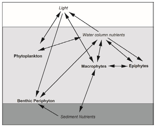
Figure 1.
Interactions among littoral primary producers (bold) and their resources (italics) in lakes. Arrows represent the directions of interactions but do not differentiate between positive or negative effects.
Establishment of IWM in littoral zones may alter biomass and production of other primary producers either by altering competition for light and nutrients, or by creating a novel growth substratum for attached algae. IWM can change the physical structures of macrophyte assemblages through altering abundances of native macrophytes [5,28]. Relative to other macrophytes, IWM does not necessarily produce more biomass, yet it can grow vertically faster and earlier than many other species [3], which allows it to shade other macrophytes and reduce their growth. Shoots of IWM have whorls of finely dissected leaves along elongated stems that have a high surface area to biomass ratio relative to other macrophyte species [29,30]. Along with high surface areas, when growing near the surface, these shoots may provide an abundant habitat with high light availability for epiphytes (but see [31]). Canopy-forming macrophytes can also decrease production by primary producers like benthic periphyton at the bottom of the water column [32,33]. Therefore, IWM presence may lead to shading of phytoplankton and benthic periphyton growing under IWM canopies, yet offer epiphytes growing attached to IWM canopies better access to light high in the water column. Because macrophytes and epiphytes can disproportionately contribute to whole-lake primary production, changes in the distribution of primary producers caused by IWM could have important consequences for energy availability and flow in lake ecosystems and food webs.
The aim of this study was to determine if IWM alters standing crops and rates of primary production by different groups of littoral primary producers. To address this question, we conducted a comparative study between plots where IWM was abundant compared to those where IWM was absent or sparse in littoral zones of six north-temperate lakes in Michigan. We measured standing crops of primary producers and their rates of primary production and respiration using bottle incubations. We also measured rates of primary production and respiration at the whole-plot scale in the littoral zone using open-water metabolism. We then applied a mass balance approach to determine the relative contributions of macrophytes, epiphytes, phytoplankton, and benthic periphyton to whole-plot primary production. This study was designed to test the following hypotheses in plots where IWM was abundant vs. those where it was absent or sparse: (1) macrophyte and epiphyte standing crops will be higher due to higher biomass and physical structure of IWM, (2) whole-plot gross primary production and ecosystem respiration rates will be higher due to higher standing crops or production of macrophytes and epiphytes, and (3) macrophytes and epiphytes will make larger contributions to whole-plot gross primary production.
2. Materials and Methods
2.1. Study Area
This field study was conducted July–September 2017 in littoral zones of 6 lakes in the Upper Peninsula and northern Lower Peninsula of Michigan (Figure 2). Waterbodies with IWM were selected based on personal observation and Michigan Invasive Species Investigation Network (MISIN) database records [34]. Additionally, waterbodies with management programs for macrophytes and IWM using herbicides were avoided unless treatments were limited in scope, and at a distance we judged would not affect our study. This was determined by checking the Michigan Department of Environment, Great Lakes and Energy’s MiWaters database [35] and personal communication with aquatic managers. In the largest waterbodies (Lake St. Helen, Sturgeon Sloughs of Portage Lake, and Islington Bay of Lake Huron) some treatments occurred, but treatment locations were not hydrologically connected to our study areas (e.g., between embayments with limited water exchange, in adjacent slough areas > 1.5 km from the selected study plots). Selected waterbodies were oligotrophic to mesotrophic and ranged in size from small inland lakes to connected waterways of the Laurentian Great Lakes (Table 1). Torch Lake was the largest and deepest lake sampled (area = 11.0 km2, mean depth 15 m), and is connected to the Keweenaw Waterway, which bisects the Keweenaw Peninsula of the Upper Peninsula and is connected to Lake Superior. Sturgeon Sloughs of Portage Lake is a complex of littoral habitat adjacent to the Sturgeon River delta also on the Keweenaw Waterway. An open bay in the Sturgeon Sloughs of Portage Lake (area of bay = 1.0 km2, mean depth 2 m) was used as a study area. Iron Lake (area = 1.6 km2, mean depth 6 m) is an inland lake in southwest Upper Peninsula and 1/10th the size of Torch Lake. Islington Bay of Lake Huron is an oligotrophic, shallow enclosed bay (area = 1.6 km2, mean depth 2 m) in the Les Cheneaux Islands region of northern Lake Huron. Horseshoe Lake is oligotrophic and the smallest inland lake included in this study (area = 0.15 km2, mean depth 3 m), located in central Lower Peninsula. Lake St. Helen is a large inland lake (area = 9.7 km2, mean depth 2 m) in central Lower Peninsula with a high percentage of littoral habitat.
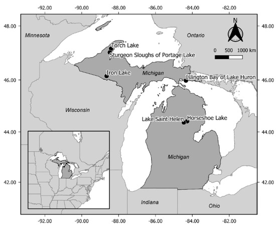
Figure 2.
Locations of waterbodies used in this study (black dots) across Michigan, USA. Coordinates of outside frame are in decimal degrees (WGS 84).

Table 1.
Locations and physical descriptions of waterbodies and study plots.
A paired-plot design was used within each waterbody to investigate the hypothesized effects of IWM on littoral zone primary producers. Circular 500-m2 plots were located in macrophyte stands based on visual presence of IWM (+IWM) and paired with a nearby plot with similar macrophyte stand structure that lacked IWM in visual surface observations during site selection (−IWM). These visual observations also indicated that IWM stems crowded the upper water column in +IWM plots of Iron Lake, Islington Bay, and Torch Lake. +IWM plots in Horseshoe Lake, Sturgeons Sloughs, and Lake St. Helen had fewer IWM stems visible in the upper water column and/or less occupied space, with other macrophytes also observed intermixed in the upper water column. It is important to note that the +IWM and −IWM labels used hereafter are based on these initial visual observations, and that detailed sampling later revealed that some −IWM plots had sparse growth of IWM, as described below.
To describe the physical and chemical properties on each sampling date, we used a YSI 6920 sonde (YSI Incorporated, Yellow Springs, OH, USA) to measure vertical profiles of temperature (°C), conductivity (mS cm−1), optical dissolved oxygen (ODO), saturation (%), and ODO concentration (mg L−1). To characterize water clarity, light extinction was determined from vertical profiles of light intensity collected with a Li-Cor LI193SA spherical underwater quantum sensor with a LI-1400 datalogger (LI-COR, Inc., Lincoln, NE, USA). A horizontal water sampler at 0.5-m depth was used to collect water for analysis of soluble reactive phosphorus (SRP), nitrate+nitrite (NO3− + NO2−), ammonium (NH4+), total dissolved nitrogen (TDN), and dissolved organic carbon (DOC). Water was immediately filtered using Millipore 0.45-µm nitrocellulose membrane filters into 60-mL bottles and placed on ice until frozen for storage in the laboratory. SRP was analyzed on a SEAL AQ2 discrete analyzer (SEAL Analytical, Mequon, WI, USA) based on USEPA method 365.1 revision 2.0 [39] and APHA method 4500-P F [40]. NO3− + NO2− was analyzed on a SEAL AQ2 discrete analyzer based on USEPA method 353.2 revision 2.0 [41] and APHA method 4500 NO3− [40]. NH4+ was analyzed using a fluorometric method [42,43] on a Turner Aquafluor (Turner Designs, Palo Alto, CA, USA). TDN and DOC samples were acidified with hydrochloric acid and quantified using a Shimadzu TOC-VCSN (Shimadzu Scientific Instruments, Columbia, MD, USA) (Table A1 in Appendix A).
2.2. Characterization of Macrophyte Assemblages
At each plot, aboveground macrophyte biomass was collected using fixed-area sampling techniques. A 16.5-cm diameter double-sided rake was lowered vertically to the lake bottom [44] and spun 1 revolution to collect a 0.0214-m2 sample of macrophytes; 20 of these samples were collected in a grid pattern across each plot to characterize plot-level standing crops. Macrophytes from each twist rake were separated and identified to species level using [45,46], and then dried at 60 °C for 48 h to constant mass to determine dry weight. Species of Chara and Drepanocladus were grouped by genera, and M. spicatum and M. spicatum x sibiricum were grouped as IWM because they are indistinguishable in the field and/or difficult to physically separate [13]. Macrophyte standing crops in each plot (total and per species, g m−2) were determined as the total dry weights divided by total area sampled in 20 twist rake samples. Dominance of IWM was quantified using two metrics. IWM standing crops were relativized to the total macrophyte standing crop of each plot (percent abundance of IWM) and standardized to the maximum standing crop measured in the dataset (standardized percent abundance of IWM).
2.3. Collection of Primary Producers for Production and Biomass
At 3 to 5 locations within each plot we collected phytoplankton, epiphytes, and benthic periphyton for production and biomass analyses. Phytoplankton were collected using a horizontal water sampler lowered to 0.5 m below the surface. Epiphytes were sampled from macrophytes growing 0.5–1 m below the water surface, typically IWM, Vallsneria americana, or Potamogeton spp. Epiphytes were collected by cutting a macrophyte stem with a razor blade and allowing it to float to the water’s surface. The stem was carefully lifted out of the water and placed into a 2-L container with 1.8 L of lake water and agitated side to side 40 times, inverting with each direction change [47]. This method removed loose epiphytes that were not tightly attached to macrophytes and created an epiphyte slurry. The stem was then removed from the 2-L container and saved for standing crop determination, as described below. Benthic periphyton were collected using a PVC sediment corer (5-cm diameter) based on a design from [48] or an Eckman grab sampler [49]. If the benthic material was a firm sediment, a modified 50-mL syringe with 2.6-cm diameter open end was pushed into the core sample to extract a subsample of the top 2 cm of benthic material. If benthic material was organic flocculent, a 50-mL syringe was used to remove the top 2 cm of the whole core sample. One-third of the flocculent material in the syringe was then used in bottle production estimates and standing crop determination.
Collection areas were determined for each primary producer to scale production and standing crop measurements to surface areas of plots, as described below. Collection areas (m2) of phytoplankton samples were calculated by dividing the respective sample volumes (m3) by depths of sampling locations (m). Epiphyte collection area (m2) was determined by measuring the dry mass (g) of macrophyte stems that were shaken for epiphyte collection as described above, and then dividing the stem dry mass by total macrophyte standing crop of each plot (g m−2). Collection area of benthic periphyton samples was the surface area of core samples extracted by syringes as described above (5.31 cm2 for benthic sediment, and 6.54 cm2 for organic flocculent material).
2.4. Bottle Production Estimates
Production estimates for phytoplankton, epiphytes, and benthic periphyton were performed by placing collected primary producers suspended in lake water into 300-mL BOD (biological oxygen demand) bottles and sealing without any air bubbles. For each primary producer group, 3 bottles were filled to determine initial concentrations of dissolved gasses (hereafter called “initial bottles”). In addition, 3 to 5 pairs of bottles were filled; then, one in each pair was tightly wrapped in heavy- duty aluminum foil (hereafter, “dark bottle”), while the other was left unaltered (hereafter, “light bottle”). Initial bottles were sampled at the start of the incubation period, while light and dark bottles were suspended for in situ incubation from a horizontal bar at sample collection depth [49,50]. Phytoplankton and epiphytes were suspended at a depth of 0.5 m below the surface. Benthic periphyton bottles were set on the bottom on hard lake bottoms, whereas on soft lake bottoms bottles were suspended 0.1 m above the bottom to prevent immersion in sediments. To account for production of phytoplankton in lake water used to suspend benthic periphyton in BOD bottles, we collected a second set of phytoplankton samples, hereafter referred to as “blanks,” that were incubated with benthic periphyton bottles. Incubation durations were based on pre-study trials to determine the optimal length that would allow detection of change in dissolved oxygen while avoiding large changes in internal bottle conditions. Based on the results of these trials, bottles with phytoplankton and blanks were incubated for 6–9 h, while bottles with epiphytes and benthic periphyton were incubated for 2–4 h.
To measure dissolved gas concentrations in all BOD bottles, triplicate water samples were collected by siphoning into 12-mL Exetainers (Labco, Lampeter, Wales, UK) and preserving with zinc chloride (0.67 g L−1 final concentration). Oxygen to argon ratios (O2:Ar) from each Exetainer were determined using membrane inlet mass spectrometry (MIMS) [51], and triplicates were averaged to calculate mean O2:Ar per bottle. For each primary producer, production rates were calculated as the change in O2:Ar ratios from the average of all initial bottles to the end of the incubation period. Net primary production (NPP) was determined from the change in light bottles, and respiration (R) from the change in dark bottles. Calculations were adapted from [49], with the addition of Ar saturation values calculated from [52] using the water temperature and barometric pressure at the time of sample collection. All rates were scaled for collection area, determined as described above, and reported in mg O2 m−2 h−1.
For each primary producer, gross primary production (GPP) was calculated as mean NPP subtracted from the mean R. Benthic periphyton GPP rates were adjusted for phytoplankton in lake water by subtracting blank GPP rates, while epiphyte GPP rates were adjusted by subtracting phytoplankton GPP rates. Propagation of standard errors from these GPP calculations followed [53,54].
2.5. Primary Producer Standing Crop Measurement
To determine standing crops of epiphytes, phytoplankton, and benthic periphyton, subsamples from each BOD bottle used for production estimates were filtered onto pre-ashed GF/F filters (0.7 μm). Filters were frozen until laboratory analysis of chlorophyll a (Chla) using ethyl alcohol extraction followed by spectrophotometric analysis with correction for phaeophytin using a Thermo Scientific 10 s UV-Vis spectrophotometer [40]. After Chla analysis, filters were analyzed for ash free dry mass (AFDM, g m−2), which provides an estimate of the total organic material in a sample and is measured as the difference between mass of the oxidized samples and initial dry mass. AFDM samples were dried at 100 °C, weighed for dry mass, and then oxidized in a muffle furnace at 550 °C, rewetted, and dried again at 100 °C before final weighing. All masses of Chla and AFDM were scaled by area of collection of the primary producer to calculate standing crops.
2.6. Open-Water Metabolism
At the center of each plot, we deployed a YSI 6920 sonde or MiniDOT logger (PME, Vista, CA, USA) in conjunction with surface mounted Hobo light and temperature pendant loggers (Onset, Bourne, MA, USA) for 3–9 days spanning the days of primary producer bottle production and standing crop sampling. All sensors were programmed to log dissolved oxygen, temperature, and light at 10-min intervals.
A modified one-station metabolism model for multiple observation days was used to estimate GPP, ecosystem respiration (ER), and air-water gas exchange [55,56]:
where GPP are positive rates and ER are negative rates of O2 production (g O2 m−2 d−1), O2 is the measured oxygen concentration (g O2 m−3), z is the depth at the location of sensor deployment (m), t is the time between measurements (d), L is irradiance, KO2 is temperature-corrected O2 gas exchange rate (d−1), and O2sat is O2 saturation concentration (g O2 m−3).
Posterior probability distributions of GPP, ER, and K were simulated using Bayesian parameter estimation with uninformative priors via a random walk Metropolis algorithm and Markov chain Monte Carlo using RSTAN 2.17.3 (Stan Development Team, https://mc-stan.org/) in R version 3.4.4 (R Core Team 2018, https://www.r-project.org/). Initially, the model was set to integrate across all measurement days to provide more robust estimates of K integrating day-to-date variability in environmental conditions [57]. Yet, when there is wide variation in weather conditions among sampling dates and/or when physical parameters override biological signals [58], these models can produce poor fits or unrealistic estimates of K, GPP, or ER. Therefore, multi-day model outputs were screened for fit and ecologically unrealistic values (negative GPP or positive ER). First, days with no or poor model fit were removed (2 days for Iron Lake −IWM, 1 day for Torch Lake +IWM, 3 days for Torch Lake −IWM). All days with ecologically unrealistic values yet good model fits (1 day for Sturgeon Sloughs −IWM, 2 days for Horseshoe Lake −IWM, 1 day for Horseshoe Lake +IWM) were additionally analyzed with single day metabolism models that estimated GPP, ER, and K from independent 24-h periods without integrating day-to-date variability of K. These single day metabolism models also produced ecologically unrealistic values for these days, so they were removed from analyses. Net ecosystem production (NEP) of plots was calculated as the sum of GPP and ER.
2.7. Production Mass Balance Estimates
We applied a mass balance approach to determine relative contributions of macrophytes, epiphytes, phytoplankton, and benthic periphyton primary production to whole-plot primary production. Hourly GPP rates (mg O2 m−2 h−1) of primary producers were first converted to daily GPP rates (g O2 m−2 d−1) by multiplying by the length of the daily photoperiod retrieved from the National Oceanic and Atmospheric Association (NOAA)’s solar calculator [59]. Primary production rates of macrophytes (GPPMacrophyte) were not directly measured; therefore, they were estimated via mass balance:
where GPPplot is the estimate of whole-plot GPP determined using open-water techniques, and GPPPhytoplankton, GPPEpiphytes, and GPPBenthic Periphyton are the daily rate of GPP for each primary producer, all in g O2 m−2 d−1.
Any negative GPP rates from bottle measurements were assumed to be due to bottle error and set to zero for these mass balance calculations, but were retained as negative values for all statistical analyses described below. This adjustment was made for benthic periphyton at Iron Lake +IWM, Islington Bay +IWM, and Lake St. Helen +IWM, and phytoplankton at Sturgeon Sloughs −IWM. When the sum of daily GPP rates of phytoplankton, epiphytes, and benthic periphyton exceeded the mean daily whole-plot GPP, this sum was used as the value for daily plot GPP, and the contribution of macrophytes was set to zero. This occurred for plots Horseshoe Lake +IWM and Iron Lake −IWM. Relative contributions of each primary producer to whole plot GPP was calculated as the daily GPP rates divided by the mean daily GPP of the plot.
2.8. Statistical Analyses
To assess the integrity of our paired plot selection, plot and water characteristics, and IWM and native macrophyte standing crops, comparisons were tested using two-sided paired t-tests in R 3.4.4. Diversity of the macrophyte assemblage was characterized as species richness and evenness, Shannon’s diversity, and Simpson’s diversity index (Table A2). These diversity metrics were calculated from a matrix composed of standing crop values of macrophytes for 12 sites × 25 species (Supplementary Materials, Table S1) in PC-ORD v6.30 (McCune, B.; Mefford, M.J. PC-ORD, Version 7.08, 2018). To describe species structure of the macrophyte assemblages across lakes and study plots we also used a non-metric multidimensional scaling (NMS) in PC-ORD v6.30, which is described in the Supplementary Materials (Tables S1–S3, Figure S1).
Comparisons of +IWM and −IWM plots were performed using paired t-tests in R 3.4.4. When testing hypotheses that macrophyte and epiphyte standing crops would be higher, plot GPP and ER rates would be higher, and macrophytes and epiphytes would make larger contributions to plot GPP in +IWM vs. −IWM plots, we used one-sided paired t-tests with the significance level set at alpha = 0.05. All other paired comparisons between +IWM and −IWM plots were performed using two-sided paired t-tests.
Stepwise multiple linear regression performed in R 3.4.4 was used to identify significant predictors of phytoplankton, epiphyte, and benthic periphyton standing crops and primary production, and to plot GPP and ER rates. Predictors initially included were light extinction, water temperature, conductivity, TDN, DOC, NH4+, SRP, NO3− + NO2−, and macrophyte standing crop. Additionally, phytoplankton Chla, epiphyte Chla, and benthic periphyton Chla were included as predictors of plot GPP. Phytoplankton AFDM, epiphyte AFDM, and benthic periphyton AFDM were included as predictors of plot ER. All variables were examined for normality and homoscedasticity; when needed variables were transformed to meet the assumptions of multiple linear regression, or variables were removed if a suitable transformation was not possible. As a result, NH4+, NO3− + NO2−, benthic periphyton Chla, epiphyte Chla, phytoplankton Chla, and benthic periphyton AFDM were logarithmically transformed for analyses. SRP was removed due to a right skewed distribution. Prior to performing regression analysis, we conducted Pearson correlation analysis to identify significant correlations (p ≤ 0.05) among predictor variables for each analysis (Supplementary Materials, Table S4). For all stepwise multiple linear regression analyses, conductivity, DOC, NH4+, and NO3− + NO2− were removed due to significant correlations with other predictor variables (Table S4). For stepwise multiple linear regression analysis of plot GPP, benthic periphyton Chla was removed due to correlation with macrophyte standing crop, and phytoplankton Chla was removed due to correlation with TDN (Table S4). Additionally, for stepwise multiple linear regression analysis of plot ER, epiphyte AFDM was removed due to correlation with phytoplankton AFDM, and benthic periphyton AFDM was removed due to correlation with macrophyte standing crop (Table S4). We identified best regression models based on the smallest Akaike’s information criteria (AIC) [60].
3. Results
3.1. Comparison of Study Sites
Site and water characteristics were similar for +IWM and −IWM plots. Plots had similar water depths (2.1 m ± 0.2 vs. 1.8 m ± 0.2, respectively, paired t-test (t values reported here and for all following), p = 0.10; Table 1 and Table 2) and all other water characteristics, including light extinction and nutrient concentrations (p ≥ 0.1, Table 2, Table A1).
Table 2.
Two-sided paired t-tests results for +IWM vs. −IWM plots.
Macrophyte assemblages differed between +IWM and −IWM plots. IWM standing crop was 50-fold higher (t = 3.69, degrees of freedom (df) = 5, p = 0.007) and total native macrophyte standing crop was 1-fold lower in +IWM vs. −IWM plots (t = −2.20, df = 5, p = 0.04), but these standing crops were variable within plots and among study lakes (Figure 3). IWM composed 61% of macrophyte biomass in +IWM plots and 2% of macrophyte biomass in −IWM plots (Table 3). The standardized abundances of IWM in +IWM plots ranged from 7% to 56%, while it was ≤ 2% in −IWM plots (Table 3). Species richness, species evenness, Shannon’s diversity, and Simpson’s diversity index were similar between +IWM and −IWM plots (Table 2, Table A2).
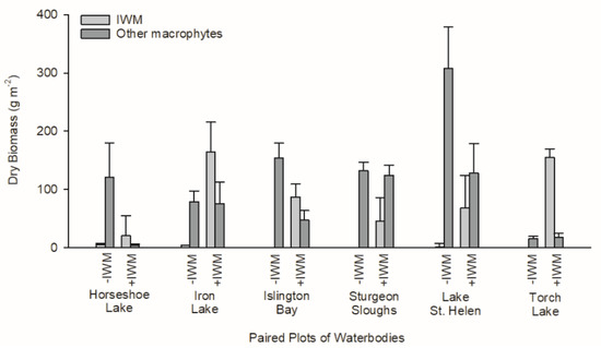
Figure 3.
Standing crops of macrophytes in paired +IWM and −IWM plots, scaled per m2 of plot surface area. “Other macrophytes” represents the sum of mean standing crops of all native macrophyte species in each plot. An error bar represents the standard error of 20 samples collected in each plot.
Table 3.
Dominance of IWM by abundance and standardized abundance in each plot.
3.2. Primary Production Rates
GPP of primary producers was not different between +IWM and −IWM plots, and across all plots GPP for benthic periphyton and phytoplankton were higher in plots with warmer water temperature. GPP rates of epiphytes, phytoplankton, and benthic periphyton were not significantly different between +IWM and −IWM plots (epiphytes, t = 0.41, df = 5, p = 0.70; phytoplankton, t = 1.44, df = 5, p = 0.21; benthic periphyton, t = −1.25, df = 5, p = 0.27) (Figure 4). Benthic periphyton GPP rates were the most variable with high standard errors (on average 56.9 ± 56.8, with SE up to 217.6 mg O2 m−2 h−1). Stepwise multiple linear regression identified significant models that explained about half of the variation in benthic periphyton and phytoplankton GPP (Table 4). Benthic periphyton GPP was negatively related to macrophyte standing crop and positively related to water temperature with R2adj = 0.50 and p = 0.02, while phytoplankton GPP was positively related to water temperature with R2adj = 0.46 and p = 0.009 (Table 4).
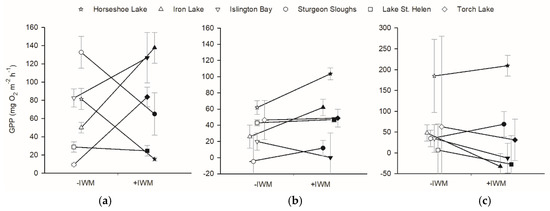
Figure 4.
Gross primary production (GPP) measured in light-dark bottles, and scaled per plot area of (a) epiphyte, (b) phytoplankton, and (c) benthic periphyton. Means ± 1 standard error are represented by symbols with error bars. Shaded symbols represent +IWM plots, and unshaded symbols represent −IWM plots for each waterbody. Lines connecting symbols illustrate differences in paired plots. Symbols are offset horizontally to aid in interpretation of error bars.
Table 4.
Stepwise multiple linear regression models selected for responses of primary producers across all plots. Best models were selected for fit and parsimony by examining Akaike information criterion (AIC) scores.
3.3. Standing Crop
Standing crops of primary producers were also not different between +IWM and −IWM plots. Total macrophyte standing crops in study plots ranged from 16.6 to 307.7 g m−2 (Figure 3). Although we hypothesized that total macrophyte biomass would be higher in +IWM plots, it was not significantly different across all plot pairs (Figure 3, t = 0.43, df = 5, p = 0.34). Additionally, epiphyte chlorophyll a (t = −0.40, df = 5, p = 0.35) and AFDM (t = −0.53, df = 5, p = 0.31) were not significantly higher in +IWM vs. −IWM plots (Figure 5). Phytoplankton Chla and AFDM were not significantly different between paired +IWM and −IWM plots (Chla, t = −0.01, df = 5, p = 0.99; AFDM, t = −1.10, df = 5, p = 0.32). Benthic periphyton Chla and AFDM were not significantly different between paired +IWM and −IWM plots (Chla, t = 0.36, df = 5, p = 0.73; AFDM, t = 0.33, df = 5, p = 0.76) (Figure 5). Benthic periphyton standing crops were generally one order of magnitude higher than phytoplankton and two orders of magnitude higher than epiphytes, as quantified by both Chla and AFDM (Figure 5). However, it should be noted that the AFDM of benthic periphyton included sediment organic matter collected in the core, and not strictly benthic periphyton.
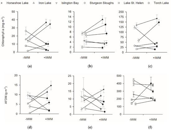
Figure 5.
Standing crops of chlorophyll a and ash free dry mass (AFDM) for (a,d) epiphyte, (b,e) phytoplankton, and (c,f) benthic periphyton. Means ± 1 SE are represented by symbols with error bars. Shaded symbols represent +IWM plots and unshaded symbols represent −IWM plots for each waterbody. Lines connecting symbols illustrate differences in paired plots. Symbols are offset horizontally to aid in interpretation of error bars.
Stepwise multiple linear regression identified significant models for Chla and AFDM of benthic periphyton and phytoplankton. Benthic periphyton Chla was positively related to water temperature and negatively related to macrophyte standing crop with R2adj = 0.49, but benthic periphyton AFDM was positively related to macrophyte standing crop and negatively related to light extinction coefficients with R2adj = 0.47 (Table 4). Phytoplankton Chla was positively related to TDN and macrophyte standing crops with R2adj = 0.65, while phytoplankton AFDM was positively related to water temperature with R2adj = 0.30 (Table 4). No significant models were produced for epiphyte Chla and AFDM (Table 4).
3.4. Open-Water Metabolism
Plot GPP and ER were not different between +IWM and −IWM plots. Plots had a wider range of ER (−2.8 to −12.5 g O2 m−2 d−1) than GPP rates (1.1 to 7.7 g O2 m−2 d−1). GPP (t = 0.62, df = 5, p = 0.28) and ER (t = 0.63, df = 5, p = 0.18) rates were not significantly higher in +IWM vs. −IWM plots (Figure 6). During time of sampling, the metabolic balance of most plots was heterotrophic, with ER greater than GPP and a range of NEP rates from 2.6 to −11.4 g O2 m−2 d−1. Stepwise multiple linear regression did not identify significant models explaining plot-level GPP and ER rates (Table 4). A model with p = 0.06 suggested that plot ER was negatively related to water temperature with R2adj = 0.25 (Table 4).
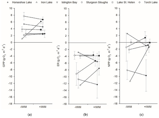
Figure 6.
Mean (a) GPP, (b) ER, and (c) net primary production (NPP) rates measured using the open-water technique and averaged over deployment periods. Means ± 1 SE are represented by symbols with error bars. Shaded symbols represent +IWM plots and unshaded symbols represent −IWM plots for each waterbody. Lines connecting symbols illustrate differences in paired plots. Symbols are offset horizontally to aid in interpretation of error bars.
3.5. Production Mass Balance Estimates
Mass balance analysis to determine the contributions of GPP from different primary producers revealed that contributions differed among lakes based on observations of IWM canopy characteristics in the study plots. Macrophytes (t = 1.35, df = 5, p = 0.23) and epiphytes (t = −0.78, df = 5, p = 0.76) did not comprise significantly higher contributions to plot GPP in +IWM vs. −IWM plots like we hypothesized they would (Figure 7). Additionally, proportions of plot GPP from phytoplankton (t = −0.32, df = 5, p = 0.76) and benthic periphyton (t = −1.18, df = 5, p = 0.29) were not significantly different between +IWM and −IWM plots. However, +IWM plots in Iron Lake, Islington Bay, and Torch Lake showed ca. 27% lower contributions to plot GPP by benthic periphyton compared to −IWM plots (Figure 7). The +IWM plots in these three waterbodies had higher standardized percentage abundances of IWM (30–56%), and dense canopies of IWM were observed while sampling, while the other +IWM plots in Horseshoe Lake, Lake St. Helen, and Sturgeon Sloughs had lower standardized percentage abundances of IWM (7–23%) and sparse upper canopies of IWM (Table 3).
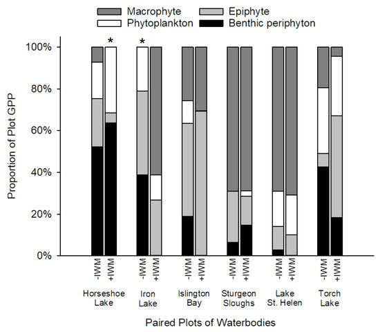
Figure 7.
Proportions of plot GPP by epiphyte, phytoplankton, benthic periphyton, and estimated macrophytes in paired +IWM and −IWM plots. Proportions of GPP from macrophytes that were set to zero are indicated with (*); see related methods in Section 2.7.
4. Discussion
We found that presence of IWM had limited effects on primary producer standing crops and rates of primary production in the littoral zones in our study of north-temperate lakes. Because we conducted this field study late in the summer, when IWM tends to reach seasonal peaks in biomass [61], we expected to find the greatest differences in standing crop and productivity between our +IWM and −IWM study plots. Contrary to our hypotheses, we found that standing crops, primary production by all primary producer groups, and plot-level GPP and ER rates were not different between our plots. However, regression analyses identified the macrophyte standing crop as a predictor of benthic periphyton GPP, epiphyte GPP, and standing crops of all other primary producers, along with water temperature, nutrient concentrations, and water clarity. These findings agree with other studies that have found that macrophyte standing crops can be an important control on whole-lake processes [17,55].
Due to the phenology and growth characteristics of IWM, we predicted that IWM would alter productivity and standing crops of primary producer groups through a suite of direct and indirect interactions (Figure 1). Other studies have documented reduced macrophyte diversity or complete displacement of native species when IWM forms dense canopies [5,6]. Yet we found that IWM was generally intermixed with native macrophytes in our study plots: IWM dominance averaged 31% of the standardized abundance of +IWM plots, and none of the +IWM plots had thick surface canopies characterized by sprawling shoots at the water’s surface. It is important to note that although we found no uniform difference in the overall macrophyte standing crops or species diversity between +IWM and −IWM plots, average standing crops of native macrophytes were 1-fold lower in +IWM plots where IWM comprised 7–56% of the standardized macrophyte abundance, compared to −IWM plots where IWM comprised 0–2%. One important caveat of our study is that the paired-plot design could obscure subtle or gradual effects of IWM density or relative abundance within or among our study lakes. For example, proportions of total production contributed by benthic periphyton GPP were ca. 27% lower in +IWM vs. −IWM plots in Torch Lake, Iron Lake, and Islington Bay (Figure 7), which were the three lakes with IWM standardized abundance ≥ 30% and dense IWM stems in the upper water column (Table 3). However, because of the paired study design, it is unclear if this pattern was driven by differences in IWM or total macrophyte biomass. Subsequent studies could employ a gradient of IWM density to more clearly separate the effects of IWM vs. overall macrophyte assemblage effects on littoral primary producers. Similarly, a gradient study could identify thresholds where IWM abundance and/or canopy structure becomes a strong control on direct and indirect interactions hypothesized in Figure 1.
Lack of IWM dominance in our study plots could be due to our study lakes being located at the northern edge of the range of IWM, where it may be limited by light and annual water temperatures [62]. Because IWM is evergreen [8], it is possible that IWM could have larger effects on macrophyte assemblages or other primary producers during times of year that were not included in our study, although we have observed strong seasonality in the absolute and relative abundance of IWM in waterbodies of this study region. In particular, greater contributions of IWM to GPP might be expected during the rapid growth phase in spring and early summer. IWM also tends to dominate under mesotrophic conditions and to flourish following disturbances [3]; these study lakes were oligo- to mesotrophic (Table A1) with no evidence of recent disturbance or active management for invasive aquatic plants near the study plots. Alternately, the low dominance of IWM in our study lakes may be consistent with the pattern that aquatic species, even invasive ones, are found in low abundances in most locations and abundant in a few [63]. For example, surveys of invasive plants of coastal wetlands of the Great Lakes found that Eurasian watermilfoil was present in 61% of lakeshore segments surveyed with an average plant community dominance of 19% [64]; for comparison, +IWM plots had an average standardized percent abundance (plant community dominance) of 31% in our study. Moreover, IWM may be similar enough to other native macrophytes in our study lakes in physical structure and nutrient uptake patterns (e.g., Ceratophyllum) that they are redundant, so that the main effects we observed were of total macrophyte standing crop on other primary producers [21,29].
Although IWM did not uniformly alter standing crop or productivity of other primary producers between plots as we hypothesized, stepwise multiple linear regression across all plots suggested that increasing macrophyte standing crop decreased benthic periphyton GPP and chla, and increased epiphyte GPP and standing crops of all other primary producers, consistent with the complex direct and indirect interactions hypothesized in Figure 1. The negative effect of macrophytes on benthic periphyton is likely a result of shading of the benthos (e.g., [65]), while positive effects of macrophytes on epiphytes and phytoplankton could be due to increases in habitat for attachment and/or changes in nutrient availability mediated by macrophytes (Figure 1) [66,67]. However, we must note that nutrient concentrations and light availability were not consistently identified as drivers of primary producer production and biomass across lakes; water clarity positively influenced benthic periphyton AFDM only. TDN was negatively associated with epiphyte GPP, chla, and AFDM, but positively associated with phytoplankton chla. The absence of these relationships could be because (1) our plot-level measurements of these water column parameters were too coarse to detect fine scale changes in light and water chemistry by macrophytes that affected interactions with other primary producers; or perhaps (2) because the macrophyte’s effects on other primary producers was due to other mechanisms, such as changes in physical habitat, patterns of water turbulence, or disturbance [15]. Water temperature was also identified as a predictor of some biomass and productivity components, which was expected, as water temperature is a primary control on many biological and physiological processes in lake ecosystems, and water temperature is controlled in lakes by regional climate, landscape characteristics, and lake morphology; we did not observe nor did we hypothesize that macrophyte presence would alter this fundamental lake characteristic (Figure 1).
The overall effects of macrophyte standing crops on other primary producers suggest that effects of IWM invasion on primary production may be stronger where IWM establishes in an area that was previously unvegetated, rather than when it replaces native species in established macrophyte stands. For example, invasions of IWM into unvegetated areas have been reported in the Tennessee Valley Association reservoirs and Lake Opinicon, Ontario [3,68]. In these situations, the creation of a macrophyte canopy where there was not one previously may be the primary effect of IWM invasion, instead of changes in the characteristics of the macrophyte assemblages. Establishment of macrophytes, whether native or non-native, can cause lake ecosystems to shift from turbid to clear water alternate stable states, with broadscale changes in the patterns of productivity, nutrient cycling, and food web dynamics that have been well studied for their importance for understanding ecological theory as well as lake management [16,69,70].
Our results suggest that in lakes where IWM is established but does not dominate macrophyte assemblages, the effects on littoral zone productivity may be minimal. Rather, overall macrophyte biomass is the primary factor controlling rates of production and biomass of other littoral zone primary producers, as has been long understood and observed in lake ecosystems. Our results agree with other studies that suggest that IWM may be functionally redundant with other macrophyte species [71], and that epiphyte assemblages do not differ significantly in composition between native and non-native macrophyte hosts [31]. In addition, our study demonstrates that littoral zone productivity is explained by factors that commonly control lake productivity across landscapes: water temperature, light availability, and nutrient supply. In conclusion, macrophyte standing crops are an important direct and indirect influence on lake processes, and invasive watermilfoil may have little impact on overall rates of primary production in these north-temperate lakes when they do not dominate the canopy within a mixed assemblage of macrophytes.
Supplementary Materials
The following are available online at https://www.mdpi.com/1424-2818/12/2/82/s1: methods and results from a non-metric multidimensional scaling analysis of the macrophyte assemblages across lakes and study plots: Table S1: Matrix of macrophyte species standing crops (g m−2) at study plots. Table S2: Reduced and logarithmic transformed matrix of macrophyte species used for NMS ordination analysis. Table S3: Correlations of macrophyte species with NMDS ordination axes. Table S4: Pairwise comparison of variables for stepwise multiple linear regressions. Figure S1: NMS ordination of paired plots in species space.
Author Contributions
This research was completed by the collaboration of authors in roles of conceptualization, R.R.V.G., A.M.M., and C.JH.; methodology, R.R.V.G. and A.M.M.; software, R.R.V.G. and A.M.M.; validation, A.M.M.; formal analysis, R.R.V.G.; investigation, R.R.V.G.; resources, R.R.V.G., A.M.M., and C.JH.; data curation, A.M.M.; writing—original draft preparation, R.R.V.G. and A.M.M.; writing—review and editing, R.R.V.G., A.M.M., and C.JH.; visualization, R.R.V.G.; supervision, A.M.M. and C.JH.; project administration, R.R.V.G. and A.M.M.; funding acquisition, R.R.V.G., A.M.M., and C.JH. All authors have read and agreed to the published version of the manuscript.
Funding
This research was funded by student fellowships to R.R.V.G. from the Midwest Aquatic Plant Management Society (Robert L. Johnson Memorial Grant), Michigan Chapter of North American Lake Management Society and Michigan Lake and Stream Associations Inc (Lake Research Grants Program), Society for Freshwater Science (Student Endowment Award), and Michigan Technological University (Ecosystem Science Center Graduate Research and Travel Grants, Great Lakes Research Center Student Research Grant). Additional funding came from U.S. Environmental Protection Agency Great Lake Restoration Initiative (assistance agreements 00E01291 and 00E01928) and Michigan Department of Natural Resources Invasive Species Grant Program (#IS14-2005).
Acknowledgments
We thank K.C. Nevorski, E.K. Eberhard, J. Pomeroy, and L. Grzelak for assistance in field sampling and lab analyses along with M. Brehob, R. Schipper, R. Kostreva, A. Norton, S. Doyle, and M. Brayden for help with lab analyses and sample processing. We thank M.A. Cavaleri, K.C. Nevorski, E.K. Eberhard, B. Wells, B. Danhoff, C. Adams, C. Brooks, T. Matthys, and two anonymous reviewers for meaningful feedback on writing and presentations. We are grateful for the facility space and boat equipment Michigan Technological University provided to support this research. This is contribution number 69 of the Great Lakes Research Center at Michigan Tech.
Conflicts of Interest
The authors declare no conflict of interest. The funders had no role in the design of the study; in the collection, analyses, or interpretation of data; in the writing of the manuscript, or in the decision to publish the results.
Appendix A
Table A1.
Water characteristics and nutrient concentrations in paired +IWM and −IWM plots.
Table A1.
Water characteristics and nutrient concentrations in paired +IWM and −IWM plots.
| Waterbody | Plot Type | Light Extinction Coefficient | Water Temperature (°C) | Conductivity (mS/cm) | SRP (µg/L) | NO3− + NO2− (µg/L) | NH4+ (µg/L) | TDN (mg/L) | DOC (mg/L) |
|---|---|---|---|---|---|---|---|---|---|
| Horseshoe Lake | −IWM | 0.563 | 23.91 | 0.244 | 0.89 | 6.0 | 18.11 | 0.444 | 7.27 |
| +IWM | 0.612 | 22.31 | 0.243 | 0.89 | 1.6 | 24.08 | 0.446 | 7.48 | |
| Lake St. Helen | −IWM | 1.277 | 22.37 | 0.179 | 0.89 | 9.0 | 9.89 | 0.542 | 14.89 |
| +IWM | 1.190 | 22.14 | 0.179 | 11.10 | 1.6 | 16.80 | 0.577 | 14.32 | |
| Islington Bay of Lake Huron | −IWM | 0.395 | 20.67 | 0.208 | 0.89 | 30.0 | 8.46 | 0.187 | 3.05 |
| +IWM | 0.366 | 20.35 | 0.209 | 2.00 | 71.0 | 6.72 | 0.218 | 3.21 | |
| Sturgeon Sloughs of Portage Lake | −IWM | 1.545 | 18.21 | 0.125 | 0.89 | 4.0 | 1.84 | 0.305 | 9.15 |
| +IWM | 0.989 | 18.98 | 0.124 | 3.10 | 46.0 | 3.99 | 0.342 | 9.17 | |
| Iron Lake | −IWM | 1.647 | 20.32 | 0.074 | 0.89 | 5.0 | 26.92 | 0.523 | 13.33 |
| +IWM | 0.990 | 20.83 | 0.073 | 0.89 | 6.0 | 12.00 | 0.533 | 11.89 | |
| Torch Lake | −IWM | 1.050 | 20.15 | 0.150 | 0.89 | 14.0 | 7.32 | 0.418 | 8.05 |
| +IWM | 0.882 | 20.99 | 0.149 | 8.10 | 71.0 | 7.64 | 0.259 | 6.70 |
Table A2.
Diversity indices of the macrophyte assemblages in paired +IWM and −IWM plots.
Table A2.
Diversity indices of the macrophyte assemblages in paired +IWM and −IWM plots.
| Waterbody | Plot Type | Species Richness | Evenness | Shannon’s Diversity Index | Simpson’s Diversity Index |
|---|---|---|---|---|---|
| Horseshoe Lake | −IWM | 6 | 0.23 | 0.44 | 0.18 |
| +IWM | 7 | 0.36 | 0.70 | 0.30 | |
| Lake St. Helen | −IWM | 8 | 0.10 | 0.21 | 0.08 |
| +IWM | 7 | 0.63 | 1.32 | 0.67 | |
| Islington Bay of Lake Huron | −IWM | 5 | 0.38 | 0.62 | 0.34 |
| +IWM | 8 | 0.55 | 1.15 | 0.54 | |
| Sturgeon Sloughs of Portage Lake | −IWM | 8 | 0.18 | 0.37 | 0.16 |
| +IWM | 11 | 0.67 | 1.61 | 0.75 | |
| Iron Lake | −IWM | 4 | 0.58 | 0.81 | 0.43 |
| +IWM | 3 | 0.69 | 0.75 | 0.46 | |
| Torch Lake | −IWM | 9 | 0.52 | 1.13 | 0.60 |
| +IWM | 8 | 0.24 | 0.50 | 0.20 |
References
- Cook, C.D.K. Worldwide distribution and taxonomy of Myriophyllum species. In Proceedings of the First International Symposium on Watermilfoil (Myriophyllum Spicatum) and Related Haloragaceae Species, Vancouver, BC, Canada, 23–24 July 1985; pp. 1–7. [Google Scholar]
- CABI Invasive Species Compendium: Myriophyllum spicatum. Available online: https://www.cabi.org/isc/datasheet/34941#2F8C4408-E2DA-4356-B1FA-98EC9FB8FFCE (accessed on 23 January 2020).
- Smith, C.S.; Barko, J.W. Ecology of Eurasian watermilfoil. J. Aquat. Plant Manag. 1990, 28, 55–64. [Google Scholar]
- Moody, M.L.; Palomino, N.; Weyl, P.S.; Coetzee, J.A.; Newman, R.M.; Harms, N.E.; Liu, X.; Thum, R.A. Unraveling the biogeographic origins of the Eurasian watermilfoil (Myriophyllum spicatum) invasion in North America. Am. J. Bot. 2016, 103, 709–718. [Google Scholar] [CrossRef]
- Madsen, J.D.; Sutherland, J.W.; Bloomfield, J.A.; Eichler, L.W.; Boylen, C.W. The decline of native vegetation under dense Eurasian watermilfoil canopies. J. Aquat. Plant Manag. 1991, 29, 94–99. [Google Scholar]
- Boylen, C.W.; Eichler, L.W.; Madsen, J.D. Loss of native plant species in a community dominated by Eurasian watermilfoil. Hydrobiologia 1999, 415, 207–211. [Google Scholar] [CrossRef]
- Madsen, J.D.; Boylen, C.W. Eurasian watermilfoil seed ecology from an oligotrophic and eutrophic lake. J. Aquat. Plant Manag. 1989, 27, 119–121. [Google Scholar]
- Nichol, S.A.; Shaw, B.H. Ecological life histories of the three aquatic nuisance plants, Myriophyllum spicatum, Potamogeton crispus and Elodea canadensis. Hydrobiologia 1986, 131, 3–21. [Google Scholar] [CrossRef]
- LaRue, E.A.; Zuellig, M.P.; Netherland, M.D.; Heilman, M.A.; Thum, R.A. Hybrid watermilfoil lineages are more invasive and less sensitive to a commonly used herbicide than their exotic parent (Eurasian watermilfoil). Evol. Appl. 2013, 462–471. [Google Scholar] [CrossRef] [PubMed]
- Parks, S.R.; McNair, J.N.; Hausler, P.; Tyning, P.; Thum, R.A. Divergent responses of cryptic invasive watermilfoil to treatment with auxinic herbicides in a large Michigan lake. Lake Reserv. Manag. 2016, 32, 366–372. [Google Scholar] [CrossRef]
- Thum, R.A.; Parks, S.; Mcnair, J.N.; Tyning, P.; Hausler, P.; Chadderton, L.; Tucker, A.; Monfils, A. Survival and vegetative regrowth of Eurasian and hybrid watermilfoil following operational treatment with auxinic herbicides in Gun Lake, Michigan. J. Aquat. Plant Manag. 2017, 55, 103–107. [Google Scholar]
- Moody, M.L.; Les, D.H. Geographic distribution and genotypic composition of invasive hybrid watermilfoil (Myriophyllum spicatum x M. sibiricum) populations in North America. Biol. Invasions 2007, 9, 559–570. [Google Scholar] [CrossRef]
- Parkinson, H.; Mangold, J.; Jacobs, J.; Madsen, J.; Halpop, J. Biology, Ecology and Management of Eurasian Watermilfoil (Myriophyllum spicatum), 2nd ed.; Montana State University Extension: Bozeman, MT, USA, 2011. [Google Scholar]
- Kovalenko, K.E.; Dibble, E.D. Invasive macrophyte effects on littoral trophic structure and carbon sources. Hydrobiologia 2014, 721, 23–34. [Google Scholar] [CrossRef]
- Carpenter, S.R.; Lodge, D.M. Effects of submerged macrophytes on ecosystem processes. Aquat. Bot. 1986, 26, 341–370. [Google Scholar] [CrossRef]
- Scheffer, M.; Hosper, S.H.; Meijer, M.L.; Moss, B.; Jeppesen, E. Alternative equilibria in shallow lakes. Trends Ecol. Evol. 1993, 8, 275–279. [Google Scholar] [CrossRef]
- Lauster, G.H.; Hanson, P.C.; Kratz, T.K. Gross primary production and respiration differences among littoral and pelagic habitats in northern Wisconsin lakes. Can. J. Fish. Aquat. Sci. 2006, 63, 1130–1141. [Google Scholar] [CrossRef]
- Binzer, T.; Sand-Jensen, K.; Middelboe, A.L. Community photosynthesis of aquatic macrophytes. Limnol. Oceanogr. 2006, 51, 2722–2733. [Google Scholar] [CrossRef]
- Barko, J.W.; Smart, R.M.; McFarland, D.G.; Chen, R.L. Interrelationships between the growth of Hydrilla verticillate (L.f.) Royle and sediment nutrient availability. Aquat. Bot. 1988, 32, 205–216. [Google Scholar] [CrossRef]
- Cattaneo, A.; Kalff, J. The relative contribution of aquatic macrophytes and their epiphytes to the production of macrophyte beds. Limnol. Oceanogr. 1980, 25, 280–289. [Google Scholar] [CrossRef]
- Barko, J.W.; Smart, R.M. Sediment-based nutrition of submersed macrophytes. Aquat. Bot. 1981, 10, 339–352. [Google Scholar] [CrossRef]
- Reuter, J.E.; Axler, R.P. Physiological characteristics of inorganic nitrogen uptake by spatially separate algal communities in a nitrogen deficient lake. Freshw. Biol. 1992, 27, 227–236. [Google Scholar] [CrossRef]
- Vadeboncoeur, Y.; Steinman, A.D. Periphyton function in lake ecosystems. Sci. World J. 2002, 2, 1449–1468. [Google Scholar] [CrossRef]
- Carignan, R.; Kalff, J. Phosphorus release by submerged macrophytes: Significance to epiphyton and phytoplankton. Limnol. Oceanogr. 1982, 27, 419–427. [Google Scholar] [CrossRef]
- Vadeboncoeur, Y.; Kalff, J.; Christofferson, K.; Jeppesen, E. Substratum as a driver of variation in periphyton chlorophyll and productivity in lakes. J. N. Am. Benthol. Soc. 2006, 25, 379–392. [Google Scholar] [CrossRef]
- Vadeboncoeur, Y.; Lodge, D.M.; Carpenter, S.R. Whole-lake fertilization effects on distribution of primary production between benthic and pelagic habitats. Ecology 2001, 82, 1065–1077. [Google Scholar] [CrossRef]
- Burkholder, J.M.; Wetzel, R.G. Epiphytic alkaline phosphatase on natural and artificial plants in an oligotrophic lake: Re-evaluation of the role of macrophytes as a phosphorus source for epiphytes. Limnol. Oceanogr. 1990, 35, 736–747. [Google Scholar] [CrossRef]
- Muthukrishnan, R.; Hansel-Welch, N.; Larkin, D.J. Environmental filtering and competitive exclusion drive biodiversity-invasibility relationships in shallow lake plant communities. J. Ecol. 2018, 106, 2058–2070. [Google Scholar] [CrossRef]
- Sher-Kaul, S.; Oertli, B.; Castella, E.; Lachavanne, J.B. Relationship between biomass and surface area of six submerged aquatic plant species. Aquat. Bot. 1995, 51, 147–154. [Google Scholar] [CrossRef]
- Dibble, E.D.; Killgore, K.J.; Dick, G.O. Measurement of plant architecture in seven aquatic plants. J. Freshw. Ecol. 1996, 11, 311–318. [Google Scholar] [CrossRef]
- Grutters, B.M.C.; Gross, E.M.; van Donk, E.; Bakker, E.S. Periphyton density is similar on native and non-native plant species. Freshw. Biol. 2017, 62, 906–915. [Google Scholar] [CrossRef]
- Lassen, C.; Revsbech, N.P.; Pederson, O. Macrophyte development and resuspension regulate the photosynthesis and production of benthic microalgae. Hydrobiologia 1997, 350, 1–11. [Google Scholar] [CrossRef]
- Vis, C.; Hudon, C.; Carignan, R. Influence of the vertical structure of macrophyte stands on epiphyte community metabolism. Can. J. Fish. Aquat. Sci. 2006, 63, 1014–1026. [Google Scholar] [CrossRef]
- Midwest Invasive Species Information Network (MISIN). Available online: https://www.misin.msu.edu/ (accessed on 1 February 2017).
- MiWaters. Available online: https://miwaters.deq.state.mi.us/miwaters/external/home (accessed on 1 February 2017).
- Navionics Chart Viewer. Available online: https://webapp.navionics.com (accessed on 18 October 2018).
- Inland Lake Maps. Available online: https://www.michigan.gov/dnr/0,4570,7-350-79119_79146_81198_85509---,00.html (accessed on 30 January 2017).
- Kerfoot, W.C.; Urban, N.R.; McDonald, C.P.; Rossman, R.; Zhang, H. Legacy mercury releases during copper mining near Lake Superior. J. Great Lakes Res. 2016, 42, 50–61. [Google Scholar] [CrossRef]
- O’Dell, J. Method 365.1, Revision 2.0: Determination of Phosphorus by Semi-Automated Colorimetry; U.S. Environmental Protection Agency, Office of Research and Development: Cincinnati, OH, USA, 1993.
- Eaton, A.D.; Clesceri, L.S.; Rice, E.W.; Greenberg, A.E.; American Public Health Association; American Water Works Association; Water Environment Federation. Standard Methods for the Examination of Water and Wastewater, 21st ed.; American Public Health Association (APHA): Washington, DC, USA, 2005. [Google Scholar]
- O’Dell, J. Method 353.2, Revision 2.0: Determination of Nitrate-Nitrite Nitrogen by Automated Colorimetry; U.S. Environmental Protection Agency, Office of Research and Development: Cincinnati, OH, USA, 1993.
- Holmes, R.M.; Aminot, A.; Kérouel, R.; Hooker, B.A.; Peterson, B.J. A simple and precise method for measuring ammonium in marine and freshwater ecosystems. Can. J. Fish. Aquat. Sci. 1999, 56, 1801–1808. [Google Scholar] [CrossRef]
- Taylor, B.W.; Keep, C.F.; Hall, R.O., Jr.; Koch, B.J.; Tronstad, L.M.; Flecker, A.S.; Ulseth, A.J. Improving the fluorometric ammonium method: Matrix effects, background fluorescence, and standard additions. J. N. Am. Benthol. Soc. 2007, 26, 167–177. [Google Scholar] [CrossRef]
- Johnson, J.A.; Newman, R.M. A comparison of two methods for sampling biomass of aquatic plants. J. Aquat. Plant Manag. 2011, 49, 1–8. [Google Scholar]
- Fasset, N.C. A Manual of Aquatic Plants, 2nd ed.; University of Wisconsin Press: Madison, WI, USA, 2006. [Google Scholar]
- Skawinksi, P.M. Aquatic Plants of the Upper Midwest: A Photographic Guide to our Underwater Forests, 2nd ed.; Paul M. Skawinski: Madison, WI, USA, 2014. [Google Scholar]
- Marcarelli, A.M.; Wurtsbaugh, W.A. Nitrogen fixation varies spatially and seasonally in linked stream-lake ecosystems. Biogeochemistry 2009, 94, 95–110. [Google Scholar] [CrossRef]
- Gardner, W.S.; McCarthy, M.J.; Carini, S.A.; Souza, A.C.; Lijun, H.; McNeal, K.S.; Puckett, M.K.; Pennington, J. Collection of intact sediment cores with overlying water to study nitrogen- and oxygen-dynamics in regions with seasonal hypoxia. Cont. Shelf Res. 2009, 29, 2207–2213. [Google Scholar] [CrossRef]
- Wetzel, R.G.; Likens, G.E. Primary productivity of phytoplankton. In Limnological Analyses, 3rd ed.; Wetzel, R.G., Likens, G.E., Eds.; Springer: New York, NY, USA, 2000; pp. 219–239. [Google Scholar]
- Vollenweider, R.A.; Talling, J.F.; Westlake, D.F. A Manual on Methods for Measuring Primary Production in Aquatic Environments; Blackwell Scientific Publications: Oxford, UK, 1974. [Google Scholar]
- Kana, T.M.; Darkangelo, C.; Hunt, M.D.; Oldham, J.B.; Bennett, G.E.; Cornwell, J.C. Membrane inlet mass spectrometer for rapid high-precision determination of N2, O2, and Ar in environmental water samples. Anal. Chem. 1994, 66, 4166–4170. [Google Scholar] [CrossRef]
- Hamme, R.C.; Emerson, S.R. The solubility of neon, nitrogen and argon in distilled water and seawater. Deep-Sea Res. Part I Oceanogr. Res. Pap. 2004, 51, 1517–1528. [Google Scholar] [CrossRef]
- Taylor, J.R. An Introduction to Error Analysis: The Study of Uncertainties in Physical Measurements, 2nd ed.; University Science Books: Sausalito, CA, USA, 1982. [Google Scholar]
- Carignan, R.; Blais, A.-M.; Vis, C. Measurement of primary production and community respiration in oligotrophic lakes using the Winkler method. Can. J. Fish. Aquat. 1998, 55, 1078–1084. [Google Scholar] [CrossRef]
- Van de Bogert, M.C.; Carpenter, S.R.; Cole, J.J.; Pace, M.L. Assessing pelagic and benthic metabolism using free water measurements. Limnol. Oceanogr. Methods 2007, 5, 145–155. [Google Scholar] [CrossRef]
- Hotchkiss, E.R.; Hall, R.O., Jr. Whole-stream 13C tracer addition reveals distinct fates of newly fixed carbon. Ecology 2015, 96, 403–416. [Google Scholar] [CrossRef] [PubMed]
- Appling, A.P.; Hall, R.O., Jr.; Yackulic, C.B.; Arroita, M. Overcoming equifinality: Leveraging long time series for stream metabolism estimation. J. Geophys. Res. Biogeosci. 2018, 123, 624–645. [Google Scholar] [CrossRef]
- Winslow, L.A.; Zwart, J.A.; Bart, R.D.; Dugan, H.A.; Woolway, R.I.; Corman, J.R.; Hanson, P.C.; Read, J.S. LakeMetabolizer: An R package for estimating lake metabolism from free-water oxygen using diverse statistical models. Inland Waters 2016, 6, 622–636. [Google Scholar] [CrossRef]
- NOAA Solar Calculator. Available online: https://www.esrl.noaa.gov/gmd/grad/solcalc/ (accessed on 8 May 2018).
- Burnham, K.P.; Anderson, D.R. Model Selection and Multimodel Inference: A Practical Information-Theoretic Approach, 2nd ed.; Springer: New York, NY, USA, 2003. [Google Scholar]
- Grace, J.B.; Wetzel, R.G. The production biology of Eurasian watermilfoil (Myriophyllum spicatum L.): A review. J. Aquat. Plant Manag. 1978, 16, 1–11. [Google Scholar]
- Madsen, J.D. Predicting the Invasion of Eurasian Watermilfoil into Northern Lakes; U.S. Army Engineer Waterways Experiment Station: Vicksburg, MS, USA, 1999. [Google Scholar]
- Hansen, G.J.; Vander Zanden, M.J.; Blum, M.J.; Clayton, M.K.; Hain, E.F.; Hauxwell, J.; Izzo, M.; Kornis, M.S.; McIntyre, P.B.; Mikulyuk, A.; et al. Commonly rare and rarely common: Comparing population abundance of invasive and native aquatic species. PLoS ONE 2013, 8, e77415. [Google Scholar] [CrossRef] [PubMed]
- Trebitz, A.S.; Taylor, D.I. Exotic and invasive aquatic plants in Great Lakes coastal wetlands: Distribution and relation to watershed land use and plant richness and cover. J. Great Lakes Res. 2007, 33, 705–721. [Google Scholar] [CrossRef]
- Sand-Jensen, K.; Borum, J. Interactions among phytoplankton, periphyton, and macrophytes in temperate freshwaters and estuaries. Aquat. Bot. 1991, 41, 137–175. [Google Scholar] [CrossRef]
- Kelly, D.J.; Hawes, I. Effects of invasive macrophytes on littoral-zone productivity and foodweb dynamics in a New Zealand high-country lake. J. N. Am. Benthol. Soc. 2005, 24, 300–320. [Google Scholar] [CrossRef]
- Ortiz, J.E.; Marcarelli, A.M.; Juneau, K.J.; Huckins, C.J. Invasive Myriophyllum spicatum and nutrients interact to influence algal assemblages. Aquat. Bot. 2019, 156, 1–9. [Google Scholar] [CrossRef]
- Keast, A. The introduced aquatic macrophyte, Myriophyllum spicatum, as habitat for fish and their invertebrate prey. Can. J. Zool. 1984, 62, 1289–1303. [Google Scholar] [CrossRef]
- Jeppsen, E.; Søndergaard, M.; Søndergaard, M.; Christoffersen, K. The Structuring Role of Submerged Macrophytes in Lakes, 1st ed.; Springer: New York, NY, USA, 1998. [Google Scholar]
- Scheffer, M. Ecology of Shallow Lakes, 1st ed.; Kluwer Academic Publishers: Dordrecht, The Netherlands, 1998. [Google Scholar]
- Schultz, R.; Dibble, E. Effects of invasive macrophytes on freshwater fish and macroinvertebrate communities: The role of invasive plant traits. Hydrobiologia 2012, 684, 1–14. [Google Scholar] [CrossRef]
© 2020 by the authors. Licensee MDPI, Basel, Switzerland. This article is an open access article distributed under the terms and conditions of the Creative Commons Attribution (CC BY) license (http://creativecommons.org/licenses/by/4.0/).