Abstract
Analysis of fluids in porous media is of great importance in many applications. There are many mathematical models that can be used in the analysis. More realistic models should account for the stochastic variations of the model parameters due to the nature of the porous material and/or the properties of the fluid. In this paper, the standard porous media problem with random permeability is considered. Both the deterministic and stochastic problems are analyzed using the finite volume technique. The solution statistics of the stochastic problem are computed using both Polynomial Chaos Expansion (PCE) and the Karhunen-Loeve (KL) decomposition with an exponential correlation function. The results of both techniques are compared with the Monte Carlo sampling to verify the efficiency. Results have shown that PCE with first order polynomials provides higher accuracy for lower (less than 20%) permeability variance. For higher permeability variance, using higher-order PCE considerably improves the accuracy of the solution. The PCE is also combined with KL decomposition and faster convergence is achieved. The KL-PCE combination should carefully choose the number of KL decomposition terms based on the correlation length of the random permeability. The suggested techniques are successfully applied to the quarter-five spot problem.
1. Introduction
Fluid flow in porous media is a subject of great interest due to its wide range of applications such as water/oil flow in underground reservoirs, modeling the underground spreading of toxic, and biological applications such as the transport in lungs and arteries [1]. When dealing with porous media, such as geological formations, we do not have complete information about their properties, such as permeability and porosity. This leads to uncertainty about the values of the formation properties and, in turn, in calculating flow in such formations [2]. For evaluating such uncertainties, a probabilistic framework is to be used. The input data are considered as random quantities, which are described in terms of stochastic processes.
Uncertainty quantification (UQ) methods are used for analyzing the system using a model by the parameterization of the uncertain input data (such as permeability) using a set of independent random variables. Then, the model is solved to determine the response of the system to the given random input data [3].
Most of the numerical models used for uncertainty quantification are based on the Monte Carlo (MC) sampling method [4,5,6,7,8,9]. This method is known for the simplicity of its implementation; however, it requires a large number of iterations of the numerical model in order to provide reliable results and therefore may be not feasible for complex simulators. In order to overcome these limitations, other variants to the standard MC method were developed such as the multilevel Monte Carlo method (MLMC) [4], Sequential Monte Carlo (SMC) Methods [5], and quasi-Monte Carlo methods [6]. In addition to the MC method and its variations, other approaches including analytical models [7] and reduced-order models [8,9] were introduced. The Karhunen-Loève (KL) expansion is an order reduction method that can be used to provide a low-dimensional representation for a Gaussian random field by performing a projection of the original system with respect to a set of spatially dependent basis and a set of independent standard normal random coefficients, where the eigenvalues and eigenvectors of the autocorrelation function of the Gaussian field are utilized in the expansion [8,9,10].
Another method is the polynomial chaos expansion (PCE) [11], where the random variables are expanded using polynomial chaos basis, then a set of equations are solved using the Galerkin technique to determine the expansion coefficients [12]. For the classical polynomial chaos expansion, the polynomial chaos basis is the Hermite polynomials, and the random variables are Gaussian. Theoretically, convergence is achieved for any functionals in the random space [13]; however, only Gaussian and near-Gaussian random fields achieve optimal convergence rate. A more general approach, the generalized polynomial chaos (gPC), was proposed in [14], where the random variables are not restricted to Gaussian random variables and the expansion is in terms of polynomials chosen from the hypergeometric polynomials of the Askey scheme [15]. However, gPC can be used only when the input pdf is known in order to choose the proper basis functions, which is not the case in many applications [16]. To overcome this issue, the arbitrary polynomial chaos (aPC) technique was proposed [16,17], where in aPC, the polynomial chaos expansion is based on the moments of the random data instead of the PDF.
When dealing with Gaussian processes, the convergence of the KL expansion is optimal [18], however, the convergence rate may be much slower for other types of processes where optimal convergence is achieved based on the particular choice, made a priori, of the basis functions used in the expansion. Therefore, PCE and KL become less accurate for nonlinear dynamics and long-time integrations due to the fixed basis and the increasing complexity with the time. To overcome that issue, the dynamically-orthogonal (DO) [19] and the bi-orthogonal (BO) [20] techniques were introduced to allow for time-dependent basis, and therefore, more accurate for long time intervals. In both techniques, the stochastic coefficients and the spatial basis evolve according to the stochastic partial differential equation (SPDE) while preserving an orthonormality conditions for the basis functions.
The purpose of this paper is to solve one of the standard porous media problems, namely, the quarter-five spot problem after imposing uncertainty to the problem. The quarter five sport problem is used to model the case when a regular set of injection and production wells is present in the reservoir; as this problem already illustrates the features and difficulties of the general problem [21]. The problem is solved using both PCE and KL techniques and the results are compared with the MC method to verify the efficiency of each technique.
2. Mathematical Statement of the Quarter-Five Spot Problem
2.1. The Deterministic Problem
Consider the problem of fluid flow in porous medium for a single-phase flow with an incompressible rock and fluid under isothermal conditions [22].
The problem is presented by the following partial differential equation (PDE):
where denotes the density of the fluid, denotes sources and sinks (out flow and in flow of fluid per unit volume), denotes the permeability, is the vertical coordinate, and is the fluid viscosity.
Let denote the downward force for gravity. Equation (1) can be expressed as
As gravity forces are approximately constant inside a reservoir domain, we get
Therefore,
where we assumed constant viscosity.
If we assume water phase with we get Equation (1) in the form
or in compact form,
where is the macroscopic Darcy velocity.
Equation (6) is a second order linear PDE. Additionally, Equation (6) is elliptic as the eigenvalues of its coefficient matrix are all negative.
2.2. The Stochastic Problem
Due to our incomplete knowledge about the medium properties, subsurface flow involves some degree of uncertainty, and therefore we need a stochastic description of the medium properties [23]. We can impose uncertainty to the quarter-five spot problem by considering the hydraulic conductivity (permeability) as a random field, where is the spatial coordinate and is the random outcome on a given probability space. This, in turn, makes the solution a random field. In our model, the boundary conditions and the source term are kept deterministic.
Thus, Equation (6) becomes an SPDE stated as
The PCE method can be used to represent a second order process , where is the space of square integrable functions, such that a random field can be expressed as [24]
To simplify writing the equations, we can eliminate the arguments when there is no ambiguity. denotes the orthogonal polynomial of degree with respect to the multidimensional random variables .
If are independent standard Gaussian random variables, then represent the multidimensional Hermite Polynomials of degree expressed as
For Gaussian random variables, Hermite polynomials are the most suitable orthogonal basis [11]. For other distributions, the basis polynomials are selected to optimize the convergence rate. This generalization is commonly known as gPC [25].
For computational purposes, if we have a random vector of dimension, then Equation (8) can be written in terms of a finite number of Hermite polynomials as
where the total number of expansion terms is determined by the random vector dimension and the order of the PCE [23].
The functions construct orthogonal basis in with the orthogonality relation [24]
where is the Kronecker delta and is the ensemble average, that is, the inner product in the Hilbert space of the variables defined by
where is the weighting function corresponding to the polynomial chaos basis .
In case that the polynomial chaos basis are the Hermite polynomials, is given by
where is the number of independent Gaussian random variables.
The mean square error of the truncated PCE expansion,, is expressed as
where is the exact solution and is the expectation operator.
For the case of univariate Gaussian stochastic germ, the following theorem provides an error bound.
Theorem 1 [25]. Given , being times continuously differentiable, the convergence rate
is obtained for an approximation of by a finite number of Hermite polynomials where the norm is induced by the inner product (14).
The KL expansion can be viewed as a special case of the PCE where only first-order polynomials have non-zero coefficients [26]. The KL expansion involves the spectral expansion of the correlation function of the process under consideration and is used to reduce the dimensionality of the random space [24]. Consider a second-order process with a correlation function. The correlation function should be real, symmetric, and positive definite [14].
We can represent as
where is a random variable, is mean of the process, a set of uncorrelated random variables, and are the eigenvalues and eigenfunctions of the correlation function, respectively, i.e.,
The KL expansion is effective when the correlation function is known, as it is characterized by an optimal convergence in the mean square sense [25]. However, the correlation function might not be known in some cases, which is a limitation of the KL expansion method.
3. Solution Implementation
3.1. The Deterministic Problem
Recall Equation (6):
To have a complete solution, we need to specify the boundary conditions. Closed flow systems where there is no fluid flow across the external boundaries are modeled by specifying homogeneous Neumann boundary conditions:
where is the normal at the boundary of the computational domain and is any spatial point that exists on the domain’s boundary .
There are several numerical methods used to solve (4), three of these methods were discussed in [22]. The first method is a cell-centered finite-volume method called the two-point flux-approximation (TPFA) scheme that is widely used in the oil industry. The TPFA scheme uses two cells pressure averages to approximate the flux across each face of the cell. In some cases, the orientation of the computational grid will affects the results of the TPFA scheme; thus, another finite-volume method called the multi-point flux-approximation (MPFA) scheme is used to overcome the inconsistencies of the TPFA scheme. Instead of using only two points such as the TPFA, the MPFA scheme utilizes each of the neighboring cell averages to approximate the flux. Another alternative to the MPFA scheme is the mixed finite-element method where the fluxes over cell edges are considered as unknowns in addition to the pressure values. However, due to the simplicity and computational speed of the TPFA, we will restrict our attention to this method. First, we write Equation (17) in the integral form inside a cell as the control volume.
To compute the flux across each face of the cell we use Darcy’s law,
where Is the interface between the two cells’ boundaries and with an area and a normal vector , is the opposite interface and has identical area but opposite normal vector.
The integral can be approximated as
where is the pressure gradient at the centroid of the interface Finite difference is used to approximate using the pressure at the interface’s centroid and the average pressure inside the cell,
where is the position vector between the center of the cell and the centroid of the interface , and is the one-sided transmissibility associated with the cell Therefore, we have for cell the relation
Similarly, we have for cell the relation
By imposing the continuity of fluxes, we have and , and after eliminating we get
where is the transmissibility associated with the connection between the two cells and . Therefore, TPFA uses the cell averages and , to approximate the flux across the interface between the cells and .
Finally, when substituting in Equation (19) we get the following system of equations,
where
Therefore we get the following system of equations,
where is a sparse, penta-diagonal symmetric matrix. Moreover, when dealing with a homogenous permeability field, is a Toeplitz matrix. The system is made positive definite, which can be effectively solved using the Cholesky decomposition algorithm [27].
Numerical Example
Equation (4) is solved on a uniform Cartesian grid covering a area with a homogeneous isotropic permeability with porosity of for all points in the grid. There is an injection well at the origin with a flow rate of 1 and 4 production wells with flow rate of −1 at the points. We use the homogeneous Neumann boundary conditions. The flow in the five-spot is symmetric about both the coordinate axes. Therefore, the domain can be reduced to a quarter of its size. This problem is called the quarter-five spot problem. Figure 1 shows the pressure distribution on the grid while illustrating the position of the injection and production wells on the bottom left and top right corners of the grid, respectively. The area of largest pressure’s value is the immediate zone surrounding the injection well (shown in red), then the pressure decreases gradually till it reaches its lowest value at the production well. In order to obtain a better view of the flow field, Pollock’s method [28] for semi-analytical tracing of streamlines is used to track the path of flow of the particles as they move from cell to cell through the cells’ centers. Additionally, traces are used, which are particles that flow with the fluid without changing the characteristics of the fluid.
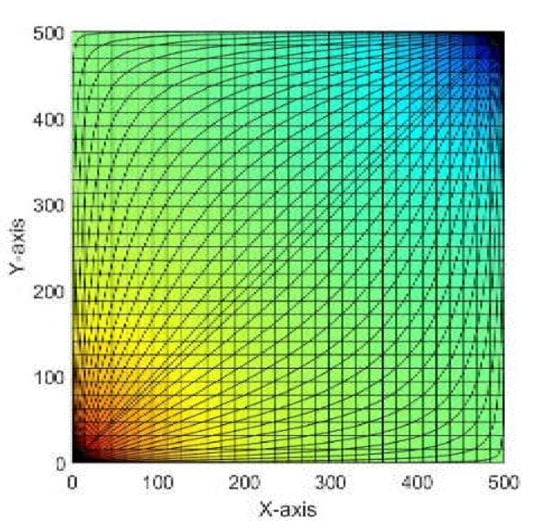
Figure 1.
Solution of the quarter-five spot problem on a uniform grid. The plot shows the pressure distribution on each point in the grid, where the highest pressure values are in the bottom left corner and the pressure decreases gradually until it reaches the lowest value at the top right corner.
The concentration of a tracer is given by a continuity equation
where is the concentration, is the inflow rate per unit volume for the tracer, and is the rock porosity. In the case of steady state flow, with tracers whose concentration do not change with fluid compression or expansion and with concentration equal to one at the inflow boundary, we get the simplified equation
We define the time-of-flight as the time required by a fluid particle to travel a given distance along a streamline. is given by the differential equation
Applying the time flight to a tracer, the communication patterns of the reservoir can be studied effectively. Therefore, in order to estimate the speed of flow inside the reservoir, we solve equation (6) subject to at the inflow to get the forward time-of-flight from inflow point and into the reservoir, and backward time-of-flight from outflow points and backwards into the reservoir. The sum of forward and backward times gives the total time required by a particle to enter the reservoir from inflow and travel through until it exits through the outflow. Figure 2 shows total travel time to illustrate the areas of high speed flow and those of stagnant flow.
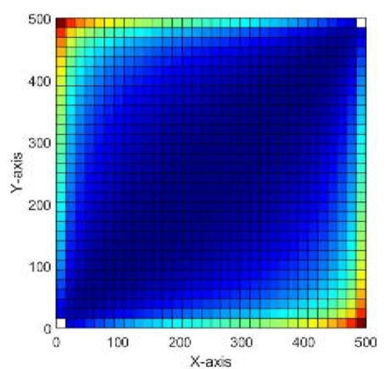
Figure 2.
Total travel time to illustrate the areas of high speed flow and those of stagnant flow.
3.2. The Stochastic Quarter-Five Spot Problem
We now proceed to solve Equation (7) while considering the uncertainty of the permeability field . The problem is first solved using only PCE, and then we will use KL expansion to reduce the dimension of the input space then apply PCE. For both scenarios, the pressure solution statistics are presented and the results are compared with the MC solution with a sample size of 10,000.
- First: Using PCE
Let permeability tensor be a random field with a Gaussian distribution of mean and variance. Consequently, the pressure vector and velocity vector become stochastic processes. In order to apply PCE, we express as a series of orthogonal basis functions (Hermite polynomials) and expansion coefficients
Accordingly,
and
substituting into Equation (7) and eliminating the arguments for brevity, we get
Which can be simplified to become
Applying inner product with each polynomial and utilizing the orthogonality relation to get a set of deterministic equations of the form
where which can be computed and stored priori [29]. We can apply the TPFA numerical scheme for this set of deterministic equations and obtain the pressure components .
- Second: Using KL expansion
As the realizations of a Gaussian distribution may take negative values, it is more practical to assume a log normal distribution for. For that purpose, first we define a Gaussian process with the KL expansion,
where is the mean, and and are the eigenvalues and eigenfunctions of the exponential correlation function , respectively. The correlation is of the form [30,31]
where denotes the spatial correlation length and is the process variance.
The permeability and are related such that is the exponential of and the PCE of would be
To obtain the coefficients , we use the formula
with given in Table 1.

Table 1.
used to evaluate the PC coefficients [11].
After computing the coefficients , we apply PCE to we get the following set of deterministic equations to be solved to get the pressure components using the TPFA scheme,
where .
4. Results
4.1. Case of PCE Only
We compare the differences in solutions obtained using MC and PCE methods. Figure 3 represents the normalized pressure mean solution produced by MC method (left) and the absolute error between the MC mean solution and the PCE mean solution (right). There was no considerable error between the two solutions (less than 0.02%) when assuming PCE with order , which proves the efficiency of the method for linear problems even when taking a low order expansion.
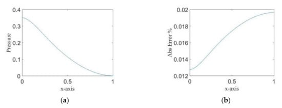
Figure 3.
(a) The pressure mean solution using MC method. (b) The percentage of difference of solutions between MC and PCE methods.
Figure 4 shows variances in pressure solutions of MC and PCE methods when eliminating one of the PCE coefficients of the input random field . It has been observed that the elimination has an insignificant impact on the accuracy of the solution. However, using more PCE coefficients tends to minimize the error between MC and PCE solutions. These results illustrate the fast convergence of the PCE solution for PDE (8), as assuming a higher-order PCE had a negligible effect on the accuracy of the solution.
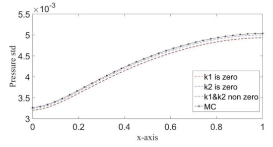
Figure 4.
Comparing the pressure standard deviation resulting from MC and PCE methods.
Table 2 illustrates the percentage of the difference between MC and PCE solutions when eliminating the first PCE coefficient, i.e., then the second PCE coefficient , then without elimination. The minimum percentage of error results when using all PCE coefficients, while using only the second PCE coefficient. resulted in more accurate results than when .
Table 2.
PCE vs. MC solution statistics.
4.2. Case of KL with PCE
In the second case, we apply the KL expansion to the input, in order to reduce the dimension of the input space and then use PCE. The permeability field is of log-normal distribution in this case. The MC method used for validation is modified by utilizing the KL expansion on a Gaussian field and constructing by taking the exponential of in every iteration.
First, we compare the convergence of the eigenvalues of the correlation function for different spatial correlation lengths. Figure 5 shows that as the correlation length decreases, the convergence would require more expansion terms. This can be further illustrated in Table 3, where the minimum number of KL terms required for convergence is provided for four different correlation lengths. We compared the solutions resulting from using PCE only and those resulting from using KL then PCE (KL-PCE) using different correlation lengths, where the results are compared against the MC solution. It has been noticed that there are no considerable differences in the mean solutions for all methods. However, the variance solution differs considerably based on the used method and the parameters and of the correlation function.
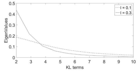
Figure 5.
Comparing Eigenvalues convergence rate for and .
Table 3.
PCE vs. MC solution statistics.
The problem is solved using PCE of order , and PCE of order after applying KL. The results show that PCE of order provides accurate results for low variance values (less than 0.5). Even for highly heterogeneous mediums where we can set
[32], PCE with first-order polynomials provides acceptable accuracy (less than 1% error when compared to MC) with no much need for higher-order PCE. However, for , using higher-order PCE is recommended for more accurate results. Therefore, we can apply KL in our problem before applying PCE as this leads to a faster convergence. It should be noted that when using KL the correlation length must be taken into consideration, as using higher correlation length would significantly reduce the accuracy of the solution if the minimum number of KL terms required for the eigenvalues convergence is not used. This can be observed in Table 4, where we compare the mean square error (MSE) percentages between MC and KL/PCE variance solutions.
Table 4.
PCE vs MC variances MSE.
5. Conclusions
In this paper, we studied the quarter-five spot problem. We solved both the deterministic problem and the stochastic problem after imposing uncertainty to the problem. We considered two cases for the stochastic problem: The first case is solved using both MC and PCE methods and the results are compared. It was shown that for the given problem, assuming a PCE with order produces an error in the mean solution less than 0.02%, while reducing the computational time to at least 30% of the time needed by the MC method. In the second case, we compared the effect of applying the KL expansion with different correlation function parameters before applying the PCE. It has been shown that for systems with low heterogeneity (low values of process variance ), PCE with first-order polynomials provides accurate results (less than 1% error). Even for a highly heterogeneous medium with PCE with first-order polynomials provides acceptable accuracy in most cases. However, if the value of increases, higher-order PCE may be required, and the KL expansion can be applied for better convergence of the PCE. When using the KL expansion, the correlation length of the correlation function should be taken into consideration before choosing the number of KL expansion terms. It was observed that a correlation function with a higher correlation length may require using the full number of KL expansion terms needed for the convergence of the eigenvalues of the correlation function. This study can be extended to predict the expected behavior of the general case when there is a system of a reservoir with injection/production wells with uncertain parameters and/or boundary conditions.
Author Contributions
H.A. was responsible for the computations, documentation and literature review. A.A.-J. was responsible for administration, supervising and reviewing the manuscript. M.E.-B. was responsible for the scientific content, novelty and analysis of the results. All authors have read and agreed to the published version of the manuscript.
Funding
This research received no external funding.
Conflicts of Interest
The authors declare no conflict of interest.
References
- Shenoy, A.V. Non-Newtonian Fluid Heat Transfer in Porous Media. In Advances in Heat Transfer; Hartnett, J.P., Irvine, T.F., Cho, Y.I., Eds.; Elsevier: Amsterdam, The Netherlands, 1994; Volume 24, pp. 101–190. [Google Scholar]
- El-Beltagy, M.A. A practical comparison between the spectral techniques in solving the SDEs. Eng. Comput. 2019, 36, 2369–2402. [Google Scholar]
- Le Maître, O.; Knio, O. Spectral Methods for Uncertainty Quantification: With Applications to Computational Fluid Dynamics; Springer Science & Business Media: Berlin/Heidelberg, Germany, 2010. [Google Scholar]
- Giles, M.B. Multilevel Monte Carlo Path Simulation. Op. Res. 2008, 56, 607–617. [Google Scholar] [CrossRef]
- Doucet, A.; de Freitas, N.; Gordon, N. An Introduction to Sequential Monte Carlo Methods. In Sequential Monte Carlo Methods in Practice; Doucet, A., de Freitas, N., Gordon, N., Eds.; Springer: New York, NY, USA, 2001; pp. 3–14. [Google Scholar]
- Caflisch, R.E. Monte Carlo and quasi-Monte Carlo methods. Acta Numer. 1998, 7, 1–49. [Google Scholar] [CrossRef]
- Gelhar, L.W. Stochastic subsurface hydrology from theory to applications. Water Resour. Res. 1986, 22, 135S–145S. [Google Scholar] [CrossRef]
- Ketabchi, H.; Ataie-Ashtiani, B. Review: Coastal groundwater optimization—advances, challenges, and practical solutions. Hydrogeol. J. 2015, 23, 1129–1154. [Google Scholar] [CrossRef]
- Razavi, S.; Tolson, B.A.; Burn, D.H. Review of surrogate modeling in water resources. Water Resour. Res. 2012, 48, W07401. [Google Scholar] [CrossRef]
- Frangos, M.; Marzouk, Y.; Willcox, K.; van Bloemen Waanders, B. Surrogate and Reduced-Order Modeling: A Comparison of Approaches for Large-Scale Statistical Inverse Problems. In Computational Methods for Large-Scale Inverse Problems and Quantification of Uncertainty; John Wiley & Sons: Hoboken, NJ, USA, 2010; pp. 123–149. [Google Scholar]
- Ghanem, R. Ingredients for a general purpose stochastic finite elements implementation. Comput. Methods Appl. Mech. Eng. 1999, 168, 19–34. [Google Scholar] [CrossRef]
- Xiu, D.; Em Karniadakis, G. Modeling uncertainty in steady state diffusion problems via generalized polynomial chaos. Comput. Methods Appl. Mech. Eng. 2002, 191, 4927–4948. [Google Scholar] [CrossRef]
- Cameron, R.H.; Martin, W.T. The Orthogonal Development of Non-Linear Functionals in Series of Fourier-Hermite Functionals. Ann. Math. 1947, 48, 385–392. [Google Scholar] [CrossRef]
- Xiu, D.; Karniadakis, G.E. The Wiener-Askey Polynomial Chaos for Stochastic Differential Equations. SIAM J. Sci. Comput. 2002, 24, 619–644. [Google Scholar] [CrossRef]
- Askey, R.; Wilson, J. Some basic hypergeometric orthogonal polynomials that generalize Jacobi polynomials. Mem. Am. Math. Soc. 1985, 54, 1–63. [Google Scholar] [CrossRef]
- Paulson, J.; Buehler, E.; Mesbah, A. Arbitrary Polynomial Chaos for Uncertainty Propagation of Correlated Random Variables in Dynamic Systems. IFAC PapersOnLine 2017, 50, 3548–3553. [Google Scholar] [CrossRef]
- Oladyshkin, S.; Nowak, W. Data-driven uncertainty quantification using the arbitrary polynomial chaos expansion. Reliab. Eng. Syst. Saf. 2012, 106, 179–190. [Google Scholar] [CrossRef]
- Loève, M. Probability Theory I; Springer: Berlin/Heidelberg, Germany, 1987. [Google Scholar]
- Sapsis, T.P.; Lermusiaux, P.F.J. Dynamically orthogonal field equations for continuous stochastic dynamical systems. Phys. D Nonlinear Phenom. 2009, 238, 2347–2360. [Google Scholar] [CrossRef]
- Cheng, M.; Hou, T.Y.; Zhang, Z. A dynamically bi-orthogonal method for time-dependent stochastic partial differential equations I: Derivation and algorithms. J. Comput. Phys. 2013, 242, 843–868. [Google Scholar] [CrossRef]
- Chavent, G.; Jaffre, J. Mathematical Models and Finite Elements in Reservoir Simulation; Elsevier: Amsterdam, The Netherlands, 1986. [Google Scholar]
- Hasle, G.; Lie, K.; Quak, E. Geometric Modelling, Numerical Simulation, and Optimization: Applied Mathematics at SINTEF; Springer: Heidelberg, Germany, 2007. [Google Scholar]
- Zhang, D. Stochastic Methods for Flow in Porous Media: Coping with Uncertainties; Academic Press: San Diego, CA, USA, 2001. [Google Scholar]
- El-Beltagy, M.A.; Wafa, M.I. Stochastic 2D incompressible Navier-Stokes solver using the vorticity-stream function formulation. J. Appl. Math. 2013, 2013, 14. [Google Scholar] [CrossRef]
- Augustin, F.; Gilg, A.; Paffrath, M.; Rentrop, P.; Wever, U. Polynomial chaos for the approximation of uncertainties: Chances and limits. Eur. J. Appl. Math. 2008, 19, 149–190. [Google Scholar] [CrossRef]
- Gentle, J.E. Numerical Linear Algebra for Applications in Statistics; Springer: Berlin/Heidelberg, Germany, 1998. [Google Scholar]
- Lie, K.-A. An Introduction to Reservoir Simulation Using MATLAB; Cambridge University Press: Cambridge, UK, 2015. [Google Scholar]
- Pollock, D.W. Semianalytical Computation of Path Lines for Finite-Difference Models. Groundwater 1988, 26, 743–750. [Google Scholar] [CrossRef]
- Noor, A.; Barnawi, A.; Nour, R.; Assiri, A.; El-Beltagy, M. Analysis of the Stochastic Population Model with Random Parameters. Entropy 2020, 22, 562. [Google Scholar] [CrossRef]
- Paleologos, E.K.; Avanidou, T.; Mylopoulos, N. Stochastic analysis and prioritization of the influence of parameter uncertainty on the predicted pressure profile in heterogeneous, unsaturated soils. J. Hazard. Mater. 2006, 136, 137–143. [Google Scholar] [CrossRef]
- Kourakos, G.; Harter, T. Parallel simulation of groundwater non-point source pollution using algebraic multigrid preconditioners. Comput. Geosci. 2014, 18, 851–867. [Google Scholar] [CrossRef]
- Crevillén-García, D.; Leung, P.K.; Rodchanarowan, A.; Shah, A.A. Uncertainty Quantification for Flow and Transport in Highly Heterogeneous Porous Media Based on Simultaneous Stochastic Model Dimensionality Reduction. Transp. Porous Media 2019, 126, 79–95. [Google Scholar] [CrossRef] [PubMed]
© 2020 by the authors. Licensee MDPI, Basel, Switzerland. This article is an open access article distributed under the terms and conditions of the Creative Commons Attribution (CC BY) license (http://creativecommons.org/licenses/by/4.0/).