Is the Finite-Time Lyapunov Exponent Field a Koopman Eigenfunction?

Abstract

This work serves as a bridge between two approaches to analysis of dynamical systems: the local, geometric analysis, and the global operator theoretic Koopman analysis. We explicitly construct vector fields where the instantaneous Lyapunov exponent field is a Koopman eigenfunction. Restricting ourselves to polynomial vector fields to make this construction easier, we find that such vector fields do exist, and we explore whether such vector fields have a special structure, thus making a link between the geometric theory and the transfer operator theory.

1. Significance

Two approaches to analyzing dynamic systems are the geometric approach and operator theoretic approach, exemplified in recent years by invariant manifolds and Koopman operators. The geometric invariant manifold approach is closely related to the instantaneous version of the finite-time Lyapunov exponent (FTLE) field. The very different, spectral and measure-based operator theoretic approach of evolution operators, also known as “Koopmanism” involves Koopman eigenfunctions (KEIGs).

In this paper, we ask a simple question, “Is the FTLE field a KEIG?” The answer is: in general, no. This motivates the explicit construction of vector fields where the answer is yes, in the sense that the FTLE field in the infinitesimal time limit, i.e., the instantaneous Lyapunov exponent (iLE) field, is a KEIG. Restricting ourselves to polynomial vector fields to make this construction easier, we indeed find that such vector fields do exist, and we explore whether such vector fields have a special structure.

2. Instantaneous Lyapunov Exponent Analysis

Solutions of non-autonomous vector fields,

$$\dot{\mathbf{x}}=\mathbf{v}(\mathbf{x},t),\mathbf{x}\in M\subset {\mathbb{R}}^n$$

(1)

such as the motion of a fluid element $\mathbf{x}\left(t\right)$ in the time-dependent fluid velocity field $\mathbf{v}(\mathbf{x},t)$, can be challenging to analyze. The method of Lagrangian coherent structures (LCS) has become a popular tool to analyze structures in the phase space of low-dimensional non-autonomous vector fields [1,2,3]. A popular computational framework to obtain LCS considers a scalar field derived from numerically integrated trajectories (i.e., numerical approximation of solutions of (1), called the “Lagrangian” point of view in the fluid literature). Specifically, the finite-time Lyapunov exponent (FTLE) field [2,4].

Recently, new tools have been developed which use vector field gradients, instead of integrating trajectories, the instantaneous time limit of FTLE and LCS. These vector gradients are assembled into the Eulerian “rate-of-strain” tensor,

$$\mathbf{S}(\mathbf{x},t)=\frac{1}{2}\left(\nabla \mathbf{v}(\mathbf{x},t)+\nabla \mathbf{v}{(\mathbf{x},t)}^T\right).$$

(2)

so-called because of its relationship to the space-fixed, or “Eulerian” point-of-view in the fluid literature. The Eulerian rate-of-strain tensor was shown to provide an instantaneous approximation of LCS in two-dimensional fluid flows [5].

Further work on this topic extended the ideas to n dimensions [6], showing that the minimum and also the maximum eigenvalues of the Eulerian rate-of-strain tensor, $s_1$ and $s_n$, are each the limits of the backward-time and forward-time FTLE fields, as the integration time goes to zero. Troughs of the field associated with the minimum eigenvalue can be identified as instantaneous attracting LCSs whereas ridges of the maximum eigenvalue field can be identified as instantaneous repelling LCSs. For the remainder of this paper, we will refer to the negatively signed minimum and positively signed maximum eigenvalues of the $\mathbf{S}$ as the attraction and repulsion rates, each, and both can be considered as instantaneous, rather than finite-time, Lyapunov exponents. For brevity we refer to the iLE field, the instantaneous Lyapunov exponent, field, following [6].

Broadly speaking, the trenches of the attraction rate field reveal where phase space regions will congregate under the flow, as shown in the schematic of Figure 1.

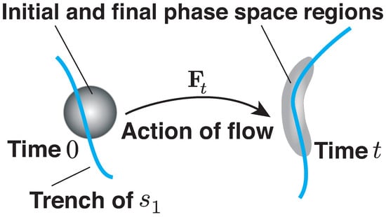
Figure 1. Schematic of the effect of the co-dimension 1 manifold, corresponding to the trench of the attraction rate, $s_1$, at an initial time, on a small parcel of phase space. The image of the trench under the time-t flow map, ${\mathbf{F}}_t$, is also shown.

These are instantaneous attracting LCSs, that is, the instantaneously most attracting co-dimension 1 surfaces in M, also referred to as instantaneous Lyapunov exponent structures (iLES) [6]. In practical applications, the primary focus has been on the attraction rate given its importance for prediction [7] as opposed to repelling features particles that will diverge from before flowing independent of those features.

In the remainder of this paper, we will restrict ourselves to autonomous systems, where the vector field (1) is independent of time, that is,

$$\dot{\mathbf{x}}=\mathbf{v}\left(\mathbf{x}\right),\mathbf{x}\in M\subset {\mathbb{R}}^n$$

(3)

2.1. Instantaneous Attraction and Repulsion Rates

For ease of exposition, we limit our discussion in this section to autonomous two-dimensional vector fields. To calculate the attraction rate, we must calculate the gradient of the vector field, $\nabla \mathbf{v}\left(\mathbf{x}\right)$, for the vector field $\mathbf{v}\left(\mathbf{x}\right)=\left(u\right(x,y),v(x,y\left)\right)$, where u is the first component and v is the second component. Additionally, the two-dimensional state is written as $\mathbf{x}=(x,y)$.

The gradient of the velocity vector is,

$$\nabla \mathbf{v}\left(\mathbf{x}\right)=\left[\begin{array}{cc}\frac{\partial u}{\partial x}& \frac{\partial u}{\partial y}\\ \frac{\partial v}{\partial x}& \frac{\partial v}{\partial y}\end{array}\right],$$

(4)

and the Eulerian rate-of-strain tensor (2) is explicitly,

$$\mathbf{S}\left(\mathbf{x}\right)=\left[\begin{array}{cc}\frac{\partial u}{\partial x}& \frac{1}{2}\left(\frac{\partial u}{\partial y}+\frac{\partial v}{\partial x}\right)\\ \frac{1}{2}\left(\frac{\partial u}{\partial y}+\frac{\partial v}{\partial x}\right)& \frac{\partial v}{\partial y}\end{array}\right].$$

(5)

The attraction rate, $s_1\left(\mathbf{x}\right)$, which is the minimum eigenvalue of $\mathbf{S}\left(\mathbf{x}\right)$ at the location $\left(\mathbf{x}\right)$ is given analytically by,

$$s_1\left(\mathbf{x}\right)=\frac{1}{2}\left(\frac{\partial u}{\partial x}+\frac{\partial v}{\partial y}\right)-\frac{1}{2}\sqrt{{\left(\frac{\partial u}{\partial x}-\frac{\partial v}{\partial y}\right)}^2+{\left(\frac{\partial u}{\partial y}+\frac{\partial v}{\partial x}\right)}^2},$$

(6)

where the dependence of u and v on $\mathbf{x}$ is understood. Similarly, the repulsion rate is given analytically by,

$$s_2\left(\mathbf{x}\right)=\frac{1}{2}\left(\frac{\partial u}{\partial x}+\frac{\partial v}{\partial y}\right)+\frac{1}{2}\sqrt{{\left(\frac{\partial u}{\partial x}-\frac{\partial v}{\partial y}\right)}^2+{\left(\frac{\partial u}{\partial y}+\frac{\partial v}{\partial x}\right)}^2},$$

(7)

2.2. Finite-Time Lyapunov Exponent

Based on the ordinary differential equation (ODE), (3), we can calculate the flow map, ${\mathbf{x}}_0\mapsto {\mathbf{x}}_t={\mathbf{F}}_t\left({\mathbf{x}}_0\right)$. The flow map, ${\mathbf{F}}_t:U\to U$, where $U\subset M$, is given by,

$${\mathbf{F}}_t\left({\mathbf{x}}_0\right)={\mathbf{x}}_0+{\int }_0^t\mathbf{v}\left({\mathbf{F}}_{\tau }\left({\mathbf{x}}_0\right)\right)d\tau ,$$

(8)

and is typically given numerically [2,8,9,10]. Taking the gradient of the flow map ${\mathbf{F}}_t\left({\mathbf{x}}_0\right)$ with respect to initial conditions ${\mathbf{x}}_0$, $\nabla {\mathbf{F}}_t\left({\mathbf{x}}_0\right)$, the right Cauchy–Green strain tensor over a time epoch of interest can be calculated,

$${\mathbf{C}}_t\left({\mathbf{x}}_0\right)=\nabla {\mathbf{F}}_t{\left({\mathbf{x}}_0\right)}^T\nabla {\mathbf{F}}_t\left({\mathbf{x}}_0\right),$$

(9)

which is positive-definite, giving eigenvalues which are all positive. In the special case of a two-dimensional flow, the resulting two eigenvalues are ordered ${\lambda }_1<{\lambda }_2$. From the maximum eigenvalue, ${\lambda }_2$, the FTLE [2,11] can be defined as,

$${\sigma }_t\left({\mathbf{x}}_0\right)=\frac{1}{2\left|t\right|}log\left({\lambda }_2\right),$$

(10)

where t is the (signed) elapsed time, often referred to as the integration time or evolution time in the FTLE literature. The FTLE measures the rate of separation of two nearby fluid parcels in a flow over the time horizon t. Ridges of the ${\sigma }_t\left({\mathbf{x}}_0\right)$ field for $t<0$ indicate regions of the flow which are the most attracting over the time interval $[t,0]$. Furthermore, in [6] it was demonstrated that the $-s_1\left({\mathbf{x}}_0\right)$ field (with the minus sign, where $s_1$ is from (6)) is the limit of the ${\sigma }_t\left({\mathbf{x}}_0\right)$ field as $t\to 0$. Thus, the attraction rate field, $s_1\left({\mathbf{x}}_0\right)$, provides a computationally inexpensive instantaneous approximation of the main attracting curves, as it is based on a single velocity snapshot; the strength is that no trajectory integration is necessary.

3. On Evolution of Observations, the Koopman Operator and Its Eigenfunction PDE

The Koopman spectral analysis has become extensively popular and relevant lately in science and engineering [12,13,14] especially for a data-driven perspective for analyzing dynamical systems. The idea is that even a non-linear dynamical system can be interpreted as a linear system, which is obviously much easier to analyze. However, this reinterpretation of the non-linear dynamical system is as a linear dynamical system in a function space, which may be infinite dimensional. The trade-off is that an infinite dimensions but linear system replaces the low-dimensional non-linear system. From there, computational schemes proceed to estimate the representation in terms of finite dimensional truncation of the infinite dimensional embedding. Often, by finite truncation the linear dynamics is approximated by finite dimensional embedding to a linear subspace.

We first review Koopman spectral analysis in brief details. Consider, the autonomous differential equation in (3). As above, the flow for each time $t\in \mathbb{R}$ (or semi-flow for positive times $t\ge 0$) as a function, $\mathbf{x}\left(t\right)\equiv {\mathbf{F}}_t\left({\mathbf{x}}_0\right)$ for a trajectory starting at initial condition $\mathbf{x}\left(0\right)={\mathbf{x}}_0\in M$. There is the dynamics of the associated Koopman operator, also often called a composition operator, which describes evolution of “observables”, meaning “measurements” along the flow, [12,15]. Rather than analyzing individual trajectories in the phase space, as is classically done, observations measured as functions over the space are analyzed. These “observation functions”,

$$g:M\to \mathbb{C},$$

(11)

are elements of a space of observation functions $\mathcal{F}$. For example,

$$\mathcal{F}=L^2\left(M\right)=\{g:{\int }_M{\left|g\left(s\right)\right|}^{2}ds<\infty \},$$

(12)

is commonly used since it is especially convenient for numerical applications that utilize the inner product associated with a Hilbert space structure [12,13,14,16,17]. We will assume scalar observation functions, but multiple scalar observation functions can also be considered together, “stacked” as a composite vector-valued observation function.

The dynamics of how observation functions change over time as sampled along orbits is precisely what the Koopman operator describes, as illustrated in Figure 2. The Koopman operator, (or composition operator), [15,18,19,20], ${\mathcal{K}}_t$, associated with $F_t$, is a (semi-)flow, stated as the following composition,

$$\begin{array}{ccc}\hfill {\mathcal{K}}_t:\mathcal{F}& \to & \mathcal{F},\hfill \\ \hfill g& \mapsto & {\mathcal{K}}_t\left[g\right]\left(\mathbf{x}\right)=g\circ {\mathbf{F}}_t,\hfill \end{array}$$

(13)

on the function space $\mathcal{F}$, for each $t\in \mathbb{R}$ (or as a semi-flow if the relation only holds for $t\ge 0$). In other words, for each $\mathbf{x}$, we observe the value of an observable g not at $\mathbf{x}$, but “downstream” by some elapsed time t, at ${\mathbf{F}}_t\left(\mathbf{x}\right)$. See Figure 2. Notice that for brevity we have suppressed the starting time $t_0$ in the statement of the Koopman operator semi-flow notation, ${\mathcal{K}}_t$. A significant feature of the Koopman operator is that it is a linear operator on its domain, the function space $\mathcal{F}$, but at the cost of possibly being infinite-dimensional. It is an infinite-dimensional linear operator despite being associated with a flow ${\mathbf{F}}_t$ that evolves on a finite-dimensional space, and indeed even due to a non-linear vector field.

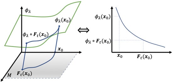
Figure 2. The action of a Koopman operator (composition operator) is to extract the value of a measurement function downstream, (Left) Equation (13), but (Right) for eigenvalue and eigenfunction pair (KEIGS) $(\lambda ,{\varphi }_{\lambda }\left(\mathbf{x}\right))$ that function has the property Equation (14) effectively interpreting the change of ${\varphi }_{\lambda }$along an orbit as if the dynamics are linear even if the flow may be non-linear in its phase space M.

The spectral theory of Koopman operators [12,15,20,21] concerns eigenfunctions and eigenvalues of the operator $K_t$. Writing an eigenvalue, eigenfunction pair of the Koopman operator as $(\lambda ,{\varphi }_{\lambda }\left(\mathbf{x}\right))$, the pair must satisfy the equation,

$${\mathcal{K}}_t\left[{\varphi }_{\lambda }\right]\left(\mathbf{x}\right)=e^{\lambda t}{\varphi }_{\lambda }\left(\mathbf{x}\right).$$

(14)

See Figure 2. For convenience, we will write “KEIGs” to refer to a Koopman eigenvalue and eigenfunction pair, $(\lambda ,{\varphi }_{\lambda }\left(\mathbf{x}\right))$. Though it may seem surprising if trying to make an analogy to the spectrum of matrices (finite rank operators), for each eigenvalue $\lambda$, the eigenfunction ${\varphi }_{\lambda }$ is not unique. In fact, there are uncountably infinitely many functions associated with each eigenvalue λ [22,23]. If one allows only unit-normalized eigenfunctions, to remove the trivial idea that constant multiples of eigenfunctions are eigenfunctions, this infinite multiplicity is still true.

An emerging concept in the empirical study of dynamical systems is the spectral decomposition of observables into eigenfunctions of the Koopman operator. Let a D-dimensional vector valued set of observables $\mathbf{g}\left(\mathbf{x}\right)=[g_1\left(\mathbf{x}\right),\dots ,g_D\left(\mathbf{x}\right)]:M\to {\mathbb{C}}^D\in {\mathcal{F}}^D,$ be written as a linear combination of eigenfunctions,

$$\mathbf{g}\left(\mathbf{x}\right)=\sum _{j=1}^{\infty }{\varphi }_{{\lambda }_j}\left(\mathbf{x}\right){\mathbf{v}}_j$$

(15)

where the vectors ${\mathbf{v}}_j\in {\mathbb{C}}^D$ are called Koopman modes. The true power of this concept lies in the following expression, which describes the dynamics of observation functions in a form reminiscent of linear Fourier analysis, but now in terms of Koopman modes. That is if, $\mathbf{y}({\mathbf{x}}_0,t)\equiv \mathbf{g}\circ \mathbf{x}\left(t\right)=\mathbf{g}\circ {\mathbf{F}}_t\left({\mathbf{x}}_0\right)=K_t\left[\mathbf{g}\right]\left({\mathbf{x}}_0\right)$, then,

$$\mathbf{y}({\mathbf{x}}_0,t)=\sum _{j=1}^{\infty }{e}^{{\lambda }_{j}t}{\varphi }_{{\lambda }_j}\left({\mathbf{x}}_0\right){\mathbf{v}}_j.$$

(16)

We considered the non-uniqueness of such a decomposition, and moreover the nature and cardinality of these eigenfunctions in [22]. In this current work, this property leads to our goal to contrast such a Koopman spectral decomposition to other notions of coherence, such as the FTLE and iLE [6]. In this way, we highlight that interesting global observation functions, such as the FTLE field, can be usefully presented as series in Koopman eigenfunctions, and in some cases, as Koopman eigenfunctions themselves.

A rapidly growing literature exists concerning data-driven approaches to construct Koopman eigenfunctions for an observed flow, given data as trajectories, namely dynamic mode decomposition, (DMD), extended dynamic mode decomposition (EDMD) and variants [24,25,26,27]. However, we will pursue an analytical description of KEIGs. This is best done in terms of a partial differential equation (PDE) which follows from the infinitesimal generator of the Koopman operator. Since the Koopman operator ${\mathcal{K}}_t$ is a semi-group of compositions, we can consider the action of the infinitesimal generator, [17,28,29],

$$\mathcal{L}=\mathbf{v}·\nabla .$$

(17)

We recall [17,28,30] that a smooth exact eigenfunction of the Koopman operator of a given flow, for a given eigenvalue $\lambda \in \mathbb{C}$ must satisfy the following PDE based on the generator (17),

$$\mathbf{v}\left(\mathbf{x}\right)·\nabla {\varphi }_{\lambda }\left(\mathbf{x}\right)=\lambda {\varphi }_{\lambda }\left(\mathbf{x}\right),$$

(18)

if M is compact, and ${\varphi }_{\lambda }:M\to \mathbb{C}$, is in $C^1\left(M\right)$, or, alternatively, if ${\varphi }_{\lambda }\in C^2\left(M\right)$. Here, we will use solutions constructed directly from (18), to compare the Koopman perspective to the LCS and iLE perspective.

This PDE is of a form that is often called quasilinear in the PDE literature [31], and, therefore, solvable by the method of characteristics, [22,23]. Note however that our specific quasilinear PDE in fact gives a linear eigenvalue problem. An initial data function $h:\Lambda \to \mathbb{C}$ propagates throughout an open domain in which the flow of the differential equation is defined, and respecting (18). That an open-KEIGS pair, $(\lambda ,{\varphi }_{\lambda }\left(\mathbf{x}\right)),{\varphi }_{\lambda }:U\subset M\to \mathbb{C}$ has the form,

$${\varphi }_{\lambda }\left(\mathbf{x}\right)=h\circ s^{*}\left(\mathbf{x}\right)e^{\lambda r^{*}\left(\mathbf{x}\right)},$$

(19)

where $r^{*}\left(\mathbf{x}\right)$ is the “time”-of-flight such that for a point $\mathbf{x}\in U$, there is an intersection in U by pull back to the data surface $\Lambda$,

$$r^{*}\left(\mathbf{x}\right)=\{r:{\mathbf{F}}_{-r}\left(\mathbf{x}\right)\cap \Lambda \ne \varnothing \}.$$

(20)

For each $\mathbf{x}\in U$,

$$s^{*}\left(\mathbf{x}\right)=s\circ {\mathbf{F}}_{-r^{*}\left(\mathbf{x}\right)}\left(\mathbf{x}\right),$$

(21)

is the parameterization on $\Lambda$ of that first intersection point. This solution is valid when the orbit is non-recurrent in the open domain, during the period of interest. In Figure 3 we illustrate schematically that a general solution of the eigenfunction PDE (18) is a pull back along the flow through $\mathbf{x}$, to read the measurement data on $\Lambda$. The measurement (observation) is then scaled according to the linear action of ${\left(e^{\lambda }\right)}^r$, for the “time” it takes to pull back the point $r=r^{*}\left(\mathbf{x}\right)$.

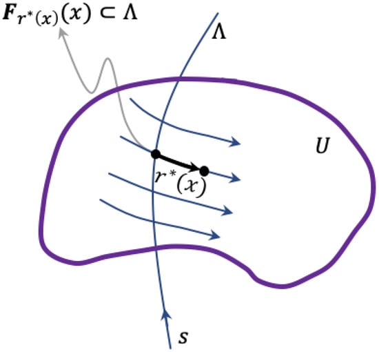
Figure 3. A general eigenfunction, that is, Equation (19) is a solution of Equation (18) is defined in terms of measuring the initial data $h\left(s\right)$ on the data surface $\Lambda$, and then for each $\mathbf{x}$ there is a unique point where that measurement is taken. Then, the solution ${\varphi }_{\lambda }$ is then a linear scaling of that measurement, by the time of the pull back.

4. One-Dimensional Vector Fields

Consider autonomous real vector fields for $x\in \mathbb{R}$,

$$\dot{x}=f\left(x\right),$$

(22)

The Eulerian rate-of-strain tensor is the one rate,

$$s_1\left(x\right)=\frac{df}{dx}\left(x\right)$$

(23)

So if $s_1\left(x\right)$ is a Koopman eigenfunction, it satisfies (18), which is,

$$\frac{d^{2}f}{d{x}^2}\left(x\right)f\left(x\right)=\lambda \frac{df}{dx}\left(x\right),$$

(24)

for some $\lambda \in \mathbb{C}$ and f. Let $g\left(x\right)=s_1\left(x\right)$ be a real scalar function, then we can state the condition as,

$$\frac{dg\left(x\right)}{dx}\int g\left(x\right)dx=\lambda g\left(x\right).$$

(25)

That is, find a function $g\left(x\right)$ such that its derivative times its integral is proportional to the function itself. We claim that the only real function $g\left(x\right)$ that satisfies this for non-zero $\lambda$ is the zero function, $g\left(x\right)=0$.

Therefore, for 1-dimensional flows, there is no non-trivial instantaneous Lyapunov exponent field which is a Koopman eigenfunction.

5. Two-Dimensional Non-Linear Saddle Flow

While in 1 dimension, the iLE field is not a Koopman eigenfunction, perhaps the situation is different in 2 dimensions. As an initial 2-dimensional vector field to motivate our study, we consider the following non-linear saddle flow which has cubic term,

$$\begin{array}{cc}\hfill \dot{x}& =x,\hfill \\ \hfill \dot{y}& =-y+y^3,\hfill \end{array}$$

(26)

in the domain $M=\{(x,y)\in {\mathbb{R}}^2|\left|y\right|<1\}$. So $\mathbf{v}\left(\mathbf{x}\right)={(x,-y+y^3)}^T$. These two uncoupled ordinary differential equations admit the explicit solutions,

$$\begin{array}{cc}\hfill x\left(t\right)& =x{e}^t,\hfill \\ \hfill y\left(t\right)& =\frac{y}{\sqrt{(1-y^2)e^{2t}+y^2}},\hfill \end{array}$$

(27)

where the initial condition at time 0 is $\mathbf{x}=(x,y)$. The right Cauchy–Green tensor for a backward integration time $t<0$, is,

$${\mathbf{C}}_t\left(\mathbf{x}\right)=\left[\begin{array}{cc}{e}^{2t}& 0\\ 0& \frac{e^{4t}}{{((1-y^2)e^{2t}+y^2)}^3}\end{array}\right],$$

(28)

which yields a backward-time FTLE ($t<0$), from (10), of,

$${\sigma }_t\left(\mathbf{x}\right)=-\frac{1}{2t}log\left(\frac{e^{4t}}{{((1-y^2)e^{2t}+y^2)}^3}\right).$$

(29)

From a Taylor series approximation for small $\left|t\right|$, the backward FTLE can be written as an expansion in t for small $\left|t\right|$,

$${\sigma }_t\left(\mathbf{x}\right)=(1-3y^2)+\mathcal{O}\left(t\right).$$

(30)

The backward-time FTLE can be approximated to leading order, $\mathcal{O}\left(1\right)$, by the negative of the minimum eigenvalue of $\mathbf{S}\left(\mathbf{x}\right)$. The matrix $\mathbf{S}\left(\mathbf{x}\right)$ is,

$$\mathbf{S}\left(\mathbf{x}\right)=\frac{1}{2}\left(\nabla \mathbf{v}+\nabla {\mathbf{v}}^T\right)=\left[\begin{array}{cc}1& 0\\ 0& (-1+3y^2)\end{array}\right]$$

(31)

The minimum eigenvalue is the iLE, the attraction rate (6), $s_1\left(\mathbf{x}\right)=-1+3y^2$.

Using $g\left(\mathbf{x}\right)=s_1\left(\mathbf{x}\right)$ as our candidate function, we find,

$$\mathbf{v}\left(\mathbf{x}\right)·\nabla g\left(\mathbf{x}\right)=6y^{2}g\left(\mathbf{x}\right)-12y^4$$

(32)

which is not in the form $\lambda g\left(\mathbf{x}\right)$ (as in (18)), so $s_1\left(\mathbf{x}\right)$ is not a Koopman eigenfunction. However, it can be written as a sum of Koopman eigenfunctions.

Following the prescription given above for constructing Koopman eigenfunction using the explicit solution (27) to the ODE, we find that the Koopman eigenfunctions are of the form,

$${\varphi }_{\lambda }\left(\mathbf{x}\right)=h\left(x\sqrt{\frac{3y^2}{1-y^2}}\right){\left(\frac{3y^2}{1-y^2}\right)}^{-\lambda /2},$$

(33)

where $h:\mathbb{R}\to \mathbb{R}$ is any scalar function of $s=x\sqrt{\frac{3y^2}{1-y^2}}$ and $\lambda \in \mathbb{C}$ is a constant. One can verify directly that a function of the form (33) satisfies (18), the infinitesimal form of the eigenvalue equation. Details are in Appendix A.

We can now construct the scalar function $s_1\left(\mathbf{x}\right)=-1+3y^2$ in terms of Koopman eigenfunctions. Note that $-1$ is a Koopman eigenfunction, using $\lambda =0$ and $h\left(s\right)=-1$, a constant function, in (33).

Additionally, note that, via Taylor series expansion, we have,

$$\frac{1}{1-y^2}=1+y^2+y^4+y^6+\mathcal{O}\left(y^8\right),$$

(34)

where $y^2<1$ due to our domain U, therefore,

$$\begin{array}{cc}\hfill {\left(\frac{3y^2}{1-y^2}\right)}^{-\frac{\lambda }{2}}={\left(3y^2\right)}^{-\frac{\lambda }{2}}& (1+(-\frac{\lambda }{2})y^2+(-\frac{\lambda }{2}+\frac{\lambda }{4}(\frac{\lambda }{2}+1))y^4\hfill \\ \hfill & +(-\frac{\lambda }{2}+\frac{\lambda }{4}(\frac{\lambda }{2}+1)-\frac{\lambda }{12}(\frac{\lambda }{2}+1)(\frac{\lambda }{2}+2))y^6+\mathcal{O}\left(y^8\right)\left)\right),\hfill \end{array}$$

(35)

Note that the following is a Koopman eigenfunction, using $\lambda =-2$ and $h\left(s\right)=1$,

$${\varphi }_{-2}\left(\mathbf{x}\right)=3y^2+3y^4+3y^6+3y^8+\mathcal{O}\left(y^{10}\right)$$

(36)

We can remove the $3y^4$ term by adding another Koopman eigenfunction, using $\lambda =-4$ and $h\left(s\right)=-\frac{1}{3}$,

$$\begin{array}{cc}\hfill {\varphi }_{-4}\left(\mathbf{x}\right)& =-\frac{1}{3}{\left(3y^2\right)}^2(1+2y^2+(2+-1(-2+1))y^4+\mathcal{O}\left(y^6\right)),\hfill \\ \hfill & =-3y^4-6y^6-9y^8+\mathcal{O}\left(y^{10}\right)\hfill \end{array}$$

(37)

We can remove the leading order remainder term from ${\varphi }_{-2}\left(\mathbf{x}\right)+{\varphi }_{-4}\left(\mathbf{x}\right)$, which is $-3y^6$, via

$$\begin{array}{cc}\hfill {\varphi }_{-6}\left(\mathbf{x}\right)& =h\left(s\right){\left(3y^2\right)}^3(1+3y^2+\mathcal{O}\left(y^4\right)),\hfill \\ \hfill & =h\left(s\right)(27y^6+81y^8+\mathcal{O}\left(y^{10}\right)).\hfill \end{array}$$

(38)

A choice of $h\left(s\right)=\frac{1}{9}$ will cancel out $-3y^6$. Following in a similar manner, we can remove the leading order remainder term from ${\varphi }_{-2}\left(\mathbf{x}\right)+{\varphi }_{-4}\left(\mathbf{x}\right)+{\varphi }_{-6}\left(\mathbf{x}\right)$, which is $3y^8$, and subsequently all higher order terms, since the leading order term of ${\varphi }_{-2k}\left(\mathbf{x}\right)$ is of order $y^{2k}$. Thus, we can write the term $3y^2$ as an infinite of Koopman eigenfunctions,

$$3y^2=\sum _{k=1}^{\infty }{\varphi }_{-2k}\left(\mathbf{x}\right),$$

(39)

where,

$${\varphi }_{-2k}\left(\mathbf{x}\right)={(-\frac{1}{3})}^{2(k-1)}{\left(\frac{3y^2}{1-y^2}\right)}^{-\frac{k}{2}},$$

(40)

for integer $k\ge 1$. Defining ${\varphi }_0\left(\mathbf{x}\right)$ as $-1$, $s_1\left(\mathbf{x}\right)$, the instantaneous attraction rate, can be written exclusively in terms of these Koopman eigenfunctions,

$$s_1\left(\mathbf{x}\right)=\sum _{k=0}^{\infty }{\varphi }_{-2k}\left(\mathbf{x}\right).$$

(41)

This simple example demonstrates that the infinitesimal FTLE, that is the iLE, is not a Koopman eigenfunction in general. However, there may be certain special case vector fields that have this property, which would imply a strong relationship between the geometric theory and the theory of evolution operators. We will consider these special vector fields in the following sections.

On the other hand, in a general scenario for a given vector field, if the corresponding eigenfunctions are dense in a space of functions that includes the iLEs, then clearly the iLE can be written as a superposition of Koopman eigenfunctions, such as described by the example above of (41). Thus, the geometric theory can still be interpreted in terms of the spectral theory. In the intermediate scenario, homogeneous polynomials (see Appendix B) offer an enticing class of problems with a general relationship. In some vector fields then, the iLE may be a finite sum of Koopman eigenfunctions.

6. General Two-Dimensional Vector Fields

Consider a general two-dimensional autonomous vector field of the form,

$$\begin{array}{cc}\hfill \dot{x}& =u(x,y),\hfill \\ \hfill \dot{y}& =v(x,y).\hfill \end{array}$$

(42)

where the right-hand-side functions u and v are as smooth as necessary in their arguments. The gradient matrix is given by (4) and the attraction and repulsion rates given by (6) and (7), respectively. We will focus on the repulsion rate, $s_2(x,y)$, but similar arguments can be applied equally to the attraction rate.

We will proceed by seeking the conditions under which $s_2(x,y)$ is also a Koopman eigenfunction for some non-trivial eigenvalue $\lambda$, which is,

$$u(x,y)\frac{\partial s_2}{\partial x}(x,y)+v(x,y)\frac{\partial s_2}{\partial y}(x,y)=\lambda s_2(x,y).$$

(43)

To simplify the calculation, we consider only vector fields, such that,

$$\frac{\partial u}{\partial y}=-\frac{\partial v}{\partial x},$$

(44)

which, in fluid terms, means the vector field has zero shear component of the strain rate [6], in which case the repulsion rate, $s_2$, in (7), simplifies to,

$$s_2=\frac{\partial u}{\partial x}.$$

(45)

with partial derivatives,

$$\frac{\partial s_2}{\partial x}=\frac{{\partial }^{2}u}{\partial x^2},\frac{\partial s_2}{\partial y}=\frac{{\partial }^{2}u}{\partial x\partial y},$$

(46)

and so the condition for the repulsion rate to be a KEIG, (43), is the following condition on the vector field functions u and v,

$$u\frac{{\partial }^{2}u}{\partial x^2}+v\frac{{\partial }^{2}u}{\partial x\partial y}=\lambda \frac{\partial u}{\partial x},$$

(47)

where the $(x,y)$ dependence of the vector field components is understood. Furthermore, under the assumption (44), the attraction rate, $s_1$, also simplifies to,

$$s_1=\frac{\partial v}{\partial y}.$$

(48)

with partial derivatives,

$$\frac{\partial s_1}{\partial x}=\frac{{\partial }^{2}v}{\partial x\partial y},\frac{\partial s_1}{\partial y}=\frac{{\partial }^{2}v}{\partial y^2},$$

(49)

and so the condition for the attraction rate to be a KEIG is the following condition on the vector field functions u and v,

$$u\frac{{\partial }^{2}v}{\partial x\partial y}+v\frac{{\partial }^{2}v}{\partial y^2}=\lambda \frac{\partial v}{\partial y}.$$

(50)

7. Polynomial Vector Fields

It is not immediately obvious if (47) or (50) admit any solutions. We seek to construct solutions, if they exist. To simplify this search, we will look initially at a special class of vector fields, polynomial vector fields.

Adopting the common notation of the polynomial vector field literature (see, e.g., [32]), we let $u(x,y)=P(x,y)$ and $v(x,y)=Q(x,y)$ be polynomials of degree m. We consider a system of the form (42) with an equilibrium point which we may place at the origin,

$$\begin{array}{cc}\hfill \dot{x}& =P_1(x,y)+P_2(x,y)+\cdots +P_m(x,y),\hfill \\ \hfill \dot{y}& =Q_1(x,y)+Q_2(x,y)+\cdots +Q_m(x,y),\hfill \end{array}$$

(51)

where $P_k(x,y)$ and $Q_k(x,y)$ are both members of $R_k$, the homogeneous polynomials of degree k (understood to be in the 2 variables x and y). The dimension of the vector space $R_k$ is equal to the number of monomials of degree k in x and y, and is, $\dim \left(R_k\right)=k+1$. The number of terms in (51) is, therefore,

$$2\sum _{k=1}^m\dim \left(R_k\right)=m(m+3).$$

(52)

We will denote the polynomials in terms of monomials,

$$P_i=\sum _{j=0}^i{a}_{ij}{x}^{i-j}{y}^j,Q_i=\sum _{j=0}^i{b}_{ij}{x}^{i-j}{y}^j,$$

(53)

where $a_{ij}$ and $b_{ij}$ are real scalar coefficients. For (51), the coefficients form a space of dimension $m(m+3)$. Based on the non-linear saddle flow example, we expect the vector fields which satisfy (47) or (50) will be some subspace of dimension $d<m(m+3)$.

7.1. Quadratic Vector Fields

Consider (51) with $m=2$,

$$\begin{array}{cc}\hfill P(x,y)& =a_{10}x+a_{11}y+a_{20}{x}^2+a_{21}xy+a_{22}{y}^2,\hfill \\ \hfill Q(x,y)& =b_{10}x+b_{11}y+b_{20}{x}^2+b_{21}xy+b_{22}{y}^2.\hfill \end{array}$$

(54)

Our assumption (44) implies,

$$\begin{array}{cc}\hfill b_{10}& =-a_{11},\hfill \\ \hfill b_{20}& =-\frac{1}{2}{a}_{21},\hfill \\ \hfill b_{21}& =-2a_{22}.\hfill \end{array}$$

(55)

Therefore, the vector fields of interest are quadratic vector fields of the form,

$$\begin{array}{cc}\hfill P(x,y)& =a_{10}x+a_{11}y+a_{20}{x}^2+a_{21}xy+a_{22}{y}^2,\hfill \\ \hfill Q(x,y)& =-a_{11}x+b_{11}y-\frac{1}{2}{a}_{21}{x}^2-2a_{22}xy+b_{22}{y}^2.\hfill \end{array}$$

(56)

which is a 7-dimensional subspace of the original 10-dimensional space of quadratic vector fields. Furthermore, for this vector field, we have,

$$s_2=\frac{\partial P}{\partial x}=a_{10}+2a_{20}x+a_{21}y,$$

(57)

and,

$$\frac{\partial s_2}{\partial x}=\frac{{\partial }^{2}P}{\partial x^2}=2a_{20},\frac{\partial s_2}{\partial y}=\frac{{\partial }^{2}P}{\partial x\partial y}=a_{21}.$$

(58)

Since $s_2$ has no second order terms, the left-hand-side of (47) must have all coefficients of second order terms identically zero, i.e.,

$$\underset{\mathrm{must}\mathrm{be}0}{\underbrace{(2a_{20}^2-\frac{1}{2}{a}_{21}^2)}}{x}^2+\underset{\mathrm{must}\mathrm{be}0}{\underbrace{(2a_{20}{a}_{21}-2a_{21}{a}_{22})}}xy+\underset{\mathrm{must}\mathrm{be}0}{\underbrace{(2a_{20}{a}_{22}+a_{21}{b}_{22})}}{y}^2=0$$

(59)

This leads to three more algebraic conditions. Among them we choose,

$$\begin{array}{cc}\hfill a_{21}& =2a_{20},\hfill \\ \hfill a_{22}& =a_{20},\hfill \\ \hfill b_{22}& =-a_{20},\hfill \end{array}$$

(60)

which reduces the space of possible vector fields to 4-dimensional.

The constant and linear terms of (47) provide the following algebraic conditions,

$$\begin{array}{cc}\hfill 0& =\lambda a_{10},\hfill \\ \hfill 2a_{20}(a_{10}-a_{11})x& =\lambda 2a_{20}x,\hfill \\ \hfill 2a_{20}(a_{11}+b_{11})y& =\lambda 2a_{20}y.\hfill \end{array}$$

(61)

This leads to conditions on $a_{10}$ and $a_{11}$,

$$\begin{array}{cc}\hfill a_{10}& =0,\hfill \\ \hfill a_{11}& =-\lambda ,\hfill \\ \hfill b_{11}& =2\lambda ,\hfill \end{array}$$

(62)

which further reduces the space of vector fields to only a 2-dimensional subspace with free parameters $(\lambda ,a_{20})$.

By construction, the repulsion rate is now a Koopman eigenfunction,

$$s_2(x,y)=2a_{20}(x+y),$$

(63)

with eigenvalue $\lambda$, where both $\lambda$ and $a_{20}$ are free parameters. The quadratic vector fields which this Koopman eigenfunction corresponds to is

$$\begin{array}{cc}\hfill P(x,y)& =-\lambda y+a_{20}{(x+y)}^2,\hfill \\ \hfill Q(x,y)& =\lambda x+2\lambda y-a_{20}{(x+y)}^2.\hfill \end{array}$$

(64)

where $(\lambda ,a_{20})\in {\mathbb{R}}^2$ are free parameters. Notice that the linear part of the vector field is skew-symmetric and that the quadratic terms in P and Q are opposite sign.

We note that while the repulsion rate $s_2=\frac{\partial P}{\partial x}$ is a KEIG, there is no guarantee that the attraction rate $s_1=\frac{\partial Q}{\partial y}$ will be.

7.2. Cubic Vector Fields

For polynomial vector fields of order m, the $s_1$ or $s_2$ fields will be polynomials of order $m-1$, since they are based on gradients of the vector field. Thus, quadratic vector fields produced a linear $s_2$ above. By the definition of an instantaneous Lyapunov exponent structure (iLES) [6], we need a ridge of $s_2$ for a repelling iLES or a trench of $s_2$ for an attracting iLES. To have this, we need an $s_1$ or $s_2$ which is quadratic. Thus, we must consider polynomial vector fields of at least cubic order.

We perform the same procedure using the same assumption (44), but now for the attraction rate, $s_1$, and for vector fields satisfying (50) which are homogeneous polynomials in x and y through order $m=3$. We augment polynomial fields of the form (51) by allowing constant terms, $P_0=a_{00}$ and $Q_0=b_{00}$, which leads to $m(m+3)+2$ terms. Out of the 20-dimensional space of planar cubic vector fields, we follow an approach analogous to the quadratic example above, and obtain,

$$\begin{array}{cc}\hfill P(x,y)& =a_{00}+a_{10}x+a_{11}y+a_{20}{(x+y)}^2+a_{20}k{(x+y)}^3,\hfill \\ \hfill Q(x,y)& =b_{00}-a_{11}x+b_{11}y-a_{20}{(x+y)}^2-a_{20}k{(x+y)}^3.\hfill \end{array}$$

(65)

where, assuming $k\ne 0$,

$$\begin{array}{cc}\hfill a_{00}& =\frac{1}{6k}\left(a_{10}-\frac{a_{20}}{3k}\right)-b_{00},\hfill \\ \hfill a_{11}& =\frac{1}{2}\left(a_{10}+\frac{a_{20}}{3k}\right),\hfill \\ \hfill b_{11}& =-\frac{a_{20}}{3k},\hfill \end{array}$$

(66)

where $(a_{10},k,a_{20},b_{00})\in {\mathbb{R}}^4$ are free parameters. Notice that the linear part of the vector field is skew-symmetric and that the quadratic and cubic terms in P and Q are opposite sign.

For this cubic vector field, the attraction rate function,

$$s_1=\frac{\partial Q}{\partial y}=-\frac{a_{20}}{3k}-2a_{20}(x+y)-3a_{20}k{(x+y)}^2,$$

(67)

is a Koopman eigenfunction with eigenvalue,

$$\lambda =a_{10}-\frac{a_{20}}{3k}.$$

(68)

Because the attraction rate field is quadratic, it can potentially have a ridge. We re-write the vector field in terms of $\lambda$ and $c=-2k{a}_{20}$,

$$\begin{array}{cc}\hfill P(x,y)& =a_{00}+(\lambda -\frac{1}{6}\frac{c}{k^2})x+(\frac{1}{2}\lambda -\frac{1}{6}\frac{c}{k^2})y-\frac{1}{2}\frac{c}{k}{(x+y)}^2-\frac{1}{2}c{(x+y)}^3,\hfill \\ \hfill Q(x,y)& =(\frac{1}{6}\frac{\lambda }{k}-a_{00})-(\frac{1}{2}\lambda -\frac{1}{6}\frac{c}{k^2})x+\frac{1}{6}\frac{c}{k^2}y+\frac{1}{2}\frac{c}{k}{(x+y)}^2+\frac{1}{2}c{(x+y)}^3,\hfill \end{array}$$

(69)

where $(\lambda ,c,k,a_{00})\in {\mathbb{R}}^4$ are free parameters. The attraction rate,

$$s_1=\frac{1}{6}\frac{c}{k^2}+\frac{c}{k}(x+y)+\frac{3}{2}c{(x+y)}^2,$$

(70)

is a Koopman eigenfunction with eigenvalue $\lambda$ for vector field (69).

7.3. Cubic Vector Field Example

As an explicit example of (69), consider the following, where $(\lambda ,c,k,a_{00})=(2,\frac{2}{3},-\frac{1}{3},-2)$,

$$\begin{array}{cc}\hfill \dot{x}& =-2+x+{(x+y)}^2-\frac{1}{3}{(x+y)}^3,\hfill \\ \hfill \dot{y}& =1+y-{(x+y)}^2+\frac{1}{3}{(x+y)}^3.\hfill \end{array}$$

(71)

The attraction rate for this vector field,

$$s_1=1-2(x+y)+{(x+y)}^2={\left((x+y)-1\right)}^2,$$

(72)

is a Koopman eigenfunction with eigenvalue $\lambda =2$. We note that if we perform a linear transformation to new variables,

$$\left[\begin{array}{c}r\\ s\end{array}\right]=T\left[\begin{array}{c}x\\ y\end{array}\right]\mathrm{where}T=\left[\begin{array}{cc}1& 1\\ -1& 1\end{array}\right],$$

(73)

we obtain a vector field that does not have the same symmetries,

$$\begin{array}{cc}\hfill \dot{r}& =-1+r,\hfill \\ \hfill \dot{s}& =3+s-2r^2+\frac{2}{3}{r}^3.\hfill \end{array}$$

(74)

but nonetheless has the same attraction rate,

$$s_1={(r-1)}^2,$$

(75)

which is a Koopman eigenfunction of the new velocity field, with the same eigenvalue $\lambda =2$.

7.4. Cubic Vector Field Transformation to Simplify

For general parameters, the same linear transformation T leads to the vector field (69) in the $(r,s)$ variables as follows,

$$\begin{array}{cc}\hfill \dot{r}& =\frac{1}{6}\frac{\lambda }{k}+\frac{1}{2}\lambda r,\hfill \\ \hfill \dot{s}& =\left(\frac{1}{6}\frac{\lambda }{k}-2a_{00}\right)+\left(-\lambda +\frac{1}{3}\frac{c}{k^2}\right)r+\frac{1}{2}\lambda s+\frac{c}{k}{r}^2+c{r}^3.\hfill \end{array}$$

(76)

As the $\dot{r}$ equation is uncoupled from s, it can be solved in closed form. For an initial condition $r_0$ at time $t_0$, we have,

$$r\left(t\right)=\frac{1}{a}\left[(\overline{a}+a{r}_0)e^{a(t-t_0)}-\overline{a}\right]$$

(77)

where $a=\frac{1}{2}\lambda$ and $\overline{a}=\frac{1}{6}\frac{\lambda }{k}$. Therefore, the s ODE can be considered a time-dependent ODE in 1D.

Notice that $\overline{r}=-\overline{a}/a=-\frac{1}{3k}$ is an invariant manifold, i.e., $\dot{r}=0$ (and this is also the location of the attraction rate iLE ridge for $k=\pm \frac{1}{3}$).

It turns out we can transform the non-linear ODE (76) into a form where it can be solved analytically. We translate the vector field so the new origin is the single equilibrium point of (76),

$$\begin{array}{cc}\hfill \overline{r}& =-\frac{1}{3k},\hfill \\ \hfill \overline{s}& =-\frac{2}{\lambda }\left(\frac{1}{2}\frac{\lambda }{k}-\frac{1}{27}\frac{c}{k^3}-2a_{00}\right),\hfill \end{array}$$

(78)

by defining,

$$\begin{array}{cc}\hfill x_1& =r-\overline{r},\hfill \\ \hfill x_2& =s-\overline{s},\hfill \end{array}$$

(79)

where the vector field in $(x_1,x_2)$ is,

$$\begin{array}{cc}\hfill {\dot{x}}_1& =\frac{\lambda }{2}{x}_1,\hfill \\ \hfill {\dot{x}}_2& =-\lambda x_1+\frac{\lambda }{2}{x}_2+c{x}_1^3.\hfill \end{array}$$

(80)

Notice this transformed system depends on only 2 parameters, $(\lambda ,c)$. Furthermore, the vector field (80) does not satisfy the simplifying assumption (44) which held in the original variables. We note that the origin of (80) is the only equilibrium point and is either a stable or unstable node, depending on whether $\lambda$ is negative or positive, respectively.

The system has an $s_1$ field that is a KEIG, ${\varphi }_{\lambda }$, with eigenvalue $\lambda$,

$$s_1=-\frac{3}{2}c{x}_1^2.$$

(81)

which has a trench at $x_1=0$ for $c<0$, which is a necessary condition for being an attracting iLES [6]. From (80), we see that the set $\{x_1=0\}$, the $x_2$-axis, is also an invariant manifold. For $\lambda <0$ $(\lambda >0)$, the $x_2$-axis is the fastest direction along the stable (unstable) invariant manifold of the origin.

7.5. Properties of KEIGs of 2-Dimensional Cubic Vector Fields

We discuss some of the properties of KEIGs of cubic vector fields in two dimensions. The ODE (80), though non-linear, is nonetheless in a form which admits Carleman linearization [33].

Augment the system with a third non-linear variable, $x_1^3$. Then, we have a linear ODE,

$$\mathbf{y}=\left[\begin{array}{c}{y}_1\\ y_2\\ y_3\end{array}\right]=\left[\begin{array}{c}{x}_1\\ x_2\\ x_2^3\end{array}\right]⟹\left[\begin{array}{c}{\dot{y}}_1\\ {\dot{y}}_2\\ {\dot{y}}_3\end{array}\right]=\underset{\mathbf{A}}{\underbrace{\left[\begin{array}{ccc}\frac{\lambda }{2}& 0& 0\\ -\lambda & \frac{\lambda }{2}& c\\ 0& 0& \frac{3}{2}\lambda \end{array}\right]}}\left[\begin{array}{c}{y}_1\\ y_2\\ y_3\end{array}\right],$$

(82)

where the $\mathbf{y}$ space can be interpreted as a three-dimensional Koopman observable vector space [34]. The linear ODE in $\mathbf{y}$ admits an analytical solution,

$$\mathbf{y}\left(t\right)=e^{\mathbf{A}t}\mathbf{y}\left(0\right),$$

(83)

which implies $x_1\left(t\right)=e^{\lambda t/2}{x}_1\left(0\right)$.

Using $s_1$ in (81) as the observable function in (13), we can explicitly find that,

$$\begin{array}{cc}\hfill s_1\left(t\right)& =-\frac{3}{2}c{x}_1{\left(t\right)}^2,\hfill \\ \hfill & =e^{\lambda t}\left(-\frac{3}{2}c{x}_1{\left(0\right)}^2\right),\hfill \\ \hfill & ={\left(e^{\lambda }\right)}^t{s}_1\left(0\right),\hfill \end{array}$$

(84)

so following individual trajectories, the $s_1$ field at time t is the same as the $s_1$ field at the initial time 0 multiplied by a factor ${\left(e^{\lambda }\right)}^t$ as we expect from an observable that is also a KEIG; see (14).

We show an example phase portrait for $(\lambda ,c)=(-1,-1)$ in Figure 4.

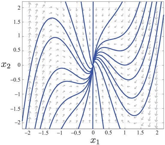
Figure 4. Phase portrait for vector field (80) in $(x_1,x_2)$ coordinates for parameters $(\lambda ,c)=(-1,-1)$. The attraction rate field for this vector field is also a Koopman eigenfunction (KEIG). The $x_2$-axis $\{x_1=0\}$, as trench of the attraction rate field, is an attracting instantaneous Lyapunov exponent structure (iLES).

For these parameters, the $x_2$-axis, $\{x_1=0\}$, is an attracting iLES.

Note that $s_1$ is not unique as a Koopman eigenfunction with eigenvalue $\lambda$. We can verify that $x_1$ is itself a KEIG with eigenvalue $\frac{\lambda }{2}$, and due to the theorem of [22], any power of $x_1$ is also a KEIG, in particular, $x_1^2$ is a KEIG with eigenvalue $\lambda$, as is $\gamma x_1^2$ for any constant $\gamma$.

7.6. A Family of Polynomial Vector Fields with a KEIG Attraction Rate

Based on the form of (80), we can construct a family of vector fields which all have the attraction rate as a KEIG,

$$\begin{array}{cc}\hfill {\dot{x}}_1& =\frac{\lambda }{2}{x}_1,\hfill \\ \hfill {\dot{x}}_2& =-\lambda x_1+\frac{\lambda }{2}{x}_2+c{x}_1^3+c_4{x}_1^4+c_5{x}_1^5+\cdots \hfill \end{array}$$

(85)

where we include in ${\dot{x}}_2$ only additional powers of $x_1$, with additional parameters $c_4$, $c_5$, etc. The vector field (85) has the attraction rate,

$$s_1=-\frac{1}{2}\left(3c{x}_1^2+4c_4{x}_1^3+5c_5{x}_1^4+\cdots \right).$$

(86)

which is a KEIG with eigenvalue $\lambda$. As before, the $x_2$-axis is (i) an attracting iLES for $c<0$ and (ii) the fastest direction along the stable (unstable) invariant manifold of the origin for $\lambda <0$ ($\lambda >0$).

8. Conclusions

In the present work, we construct vector fields with the property that either the attraction rate or repulsion rate is a Koopman eigenfunction. We find that in 1 dimension, this is not possible, but in 2 dimensions, it is. We consider cubic 2-dimensional vector fields, and find a 2-parameter family of systems which have an attraction rate KEIG. It turns out that these systems, while non-linear, have the unusual property that Carleman linearization truncates at finite order, allowing us to find the exact analytical solution of the flow map using linear methods. It is not obvious why the search for a vector field where the attraction rate is a KEIG would lead to this property.

The further investigation of vector fields which have attraction and repulsion rate fields as KEIGs is left as future work. Returning to the title question of this paper, “Is the finite-time Lyapunov exponent field a Koopman eigenfunction?” while the answer is yes in some special cases, in general, the answer is no.

References

- Haller, G.; Yuan, G. Lagrangian coherent structures and mixing in two-dimensional turbulence. Physical D 2000, 147, 352–370. [Google Scholar] [CrossRef]
- Shadden, S.C.; Lekien, F.; Marsden, J.E. Definition and properties of Lagrangian coherent structures from finite-time Lyapunov exponents in two-dimensional aperiodic flows. Phys. D Nonlinear Phenom. 2005, 212, 271–304. [Google Scholar] [CrossRef]
- Haller, G. Lagrangian Coherent Structures. Annu. Rev. Fluid Mech. 2015, 47, 137–162. [Google Scholar] [CrossRef] [Green Version]
- Lekien, F.; Ross, S.D. The computation of finite-time Lyapunov exponents on unstructured meshes and for non-Euclidean manifolds. Chaos Interdiscip. J. Nonlinear Sci. 2010, 20, 017505. [Google Scholar] [CrossRef] [Green Version]
- Serra, M.; Haller, G. Objective Eulerian coherent structures. Chaos Interdiscip. J. Nonlinear Sci. 2016, 26, 053110. [Google Scholar] [CrossRef] [Green Version]
- Nolan, P.J.; Serra, M.; Ross, S.D. Finite-time Lyapunov exponents in the instantaneous limit and material transport. Nonlinear Dyn. 2020, 100, 3825–3852. [Google Scholar] [CrossRef]
- Nolan, P.J.; Pinto, J.; González-Rocha, J.; Jensen, A.; Vezzi, C.; Bailey, S.; de Boer, G.; Diehl, C.; Laurence, R.; Powers, C.; et al. Coordinated unmanned aircraft system (UAS) and ground-based weather measurements to predict Lagrangian coherent structures (LCSs). Sensors 2018, 18, 4448. [Google Scholar] [CrossRef] [PubMed] [Green Version]
- Brunton, S.L.; Rowley, C.W. Fast computation of FTLE fields for unsteady flows: A comparison of methods. Chaos Interdiscip. J. Nonlinear Sci. 2010, 20, 017503. [Google Scholar] [CrossRef]
- Rypina, I.I.; Scott, S.; Pratt, L.J.; Brown, M.G. Investigating the connection between complexity of isolated trajectories and Lagrangian coherent structures. Nonlinear Process. Geophys. 2011, 18, 977–987. [Google Scholar] [CrossRef]
- Pratt, L.J.; Rypina, I.I.; Özgökmen, T.M.; Wang, P.; Childs, H.; Bebieva, Y. Chaotic advection in a steady, three-dimensional, Ekman-driven eddy. J. Fluid Mech. 2014, 738, 143–183. [Google Scholar] [CrossRef] [Green Version]
- Lekien, F.; Shadden, S.C.; Marsden, J.E. Lagrangian coherent structures in n-dimensional systems. J. Math. Phys. 2007, 48, 065404. [Google Scholar] [CrossRef]
- Budišić, M.; Mohr, R.; Mezić, I. Applied Koopmanism. Chaos Interdiscip. J. Nonlinear Sci. 2012, 22, 047510. [Google Scholar] [CrossRef] [Green Version]
- Kutz, J.N.; Brunton, S.L.; Brunton, B.W.; Proctor, J.L. Dynamic Mode Decomposition: Data-Driven Modeling of Complex Systems; SIAM: Philadelphia, PA, USA, 2016. [Google Scholar]
- Lan, Y.; Mezić, I. Linearization in the large of nonlinear systems and Koopman operator spectrum. Phys. D Nonlinear Phenom. 2013, 242, 42–53. [Google Scholar] [CrossRef]
- Mezić, I. Analysis of fluid flows via spectral properties of the Koopman operator. Annu. Rev. Fluid Mech. 2013, 45, 357–378. [Google Scholar] [CrossRef] [Green Version]
- Mezić, I. Spectral properties of dynamical systems, model reduction and decompositions. Nonlinear Dyn. 2005, 41, 309–325. [Google Scholar] [CrossRef]
- Mezić, I. Spectrum of the Koopman operator, spectral expansions in functional spaces, and state-space geometry. J. Nonlinear Sci. 2020, 30, 2091–2145. [Google Scholar] [CrossRef] [Green Version]
- Koopman, B.O. Hamiltonian systems and transformation in Hilbert space. Proc. Natl. Acad. Sci. USA 1931, 17, 315. [Google Scholar] [CrossRef] [Green Version]
- Cvitanovic, P.; Artuso, R.; Mainieri, R.; Tanner, G.; Vattay, G.; Whelan, N.; Wirzba, A. Chaos: Classical and Quantum. Chaosbook.Org; Niels Bohr Institute: Copenhagen, Denmark, 2005. [Google Scholar]
- Gaspard, P. Chaos, Scattering and Statistical Mechanics; Cambridge University Press: Cambridge, UK, 2005; Volume 9. [Google Scholar]
- Mauroy, A.; Mezić, I. Global stability analysis using the eigenfunctions of the Koopman operator. IEEE Trans. Autom. Control. 2016, 61, 3356–3369. [Google Scholar] [CrossRef] [Green Version]
- Bollt, E.M. Geometric considerations of a good dictionary for Koopman analysis of dynamical systems: Cardinality, “primary eigenfunction”, and efficient representation. Commun. Nonlinear Sci. Numer. Simul. 2021, 100, 105833. [Google Scholar] [CrossRef]
- Korda, M.; Mezić, I. Optimal construction of Koopman eigenfunctions for prediction and control. IEEE Trans. Autom. Control 2020, 65, 5114–5129. [Google Scholar] [CrossRef] [Green Version]
- Schmid, P.J. Dynamic mode decomposition of numerical and experimental data. J. Fluid Mech. 2010, 656, 5–28. [Google Scholar] [CrossRef] [Green Version]
- Williams, M.O.; Kevrekidis, I.G.; Rowley, C.W. A Data-Driven Approximation of the Koopman Operator: Extending Dynamic Mode Decomposition. J. Nonlinear Sci. 2015, 25, 1307–1346. [Google Scholar] [CrossRef] [Green Version]
- Williams, M.O.; Rowley, C.W.; Mezić, I.; Kevrekidis, I.G. Data fusion via intrinsic dynamic variables: An application of data-driven Koopman spectral analysis. EPL (Europhys. Lett.) 2015, 109, 40007. [Google Scholar] [CrossRef] [Green Version]
- Li, Q.; Dietrich, F.; Bollt, E.M.; Kevrekidis, I.G. Extended dynamic mode decomposition with dictionary learning: A data-driven adaptive spectral decomposition of the Koopman operator. Chaos Interdiscip. J. Nonlinear Sci. 2017, 27, 103111. [Google Scholar] [CrossRef] [PubMed]
- Lasota, A.; Mackey, M.C. Chaos, Fractals, and Noise: Stochastic Aspects of Dynamics; Springer Science & Business Media: Berlin, Germany, 2013; Volume 97. [Google Scholar]
- Bollt, E.M.; Santitissadeekorn, N. Applied and Computational Measurable Dynamics; SIAM: Philadelphia, PA, USA, 2013. [Google Scholar]
- Bollt, E.M.; Li, Q.; Dietrich, F.; Kevrekidis, I. On matching, and even rectifying, dynamical systems through Koopman operator eigenfunctions. SIAM J. Appl. Dyn. Syst. 2018, 17, 1925–1960. [Google Scholar] [CrossRef]
- John, F. Partial Differential Equations; Springer: Berlin, Germany, 1975. [Google Scholar]
- Schlomiuk, D. Algebraic and geometric aspects of the theory of polynomial vector fields. In Bifurcations and Periodic Orbits of Vector Fields; Springer: Berlin, Germany, 1993; pp. 429–467. [Google Scholar]
- Carleman, T. Applications de la théore des équations intégral singulières aux équations différentielles de la dynamique. T. Ark. Mat. Astron. Fys. 1932, 22B, 1–7. [Google Scholar]
- Brunton, S.L.; Kutz, J.N. Data-Driven Science and Engineering: Machine Learning, Dynamical Systems, and Control; Cambridge University Press: Cambridge, UK, 2019. [Google Scholar]
Publisher’s Note: MDPI stays neutral with regard to jurisdictional claims in published maps and institutional affiliations. |
© 2021 by the authors. Licensee MDPI, Basel, Switzerland. This article is an open access article distributed under the terms and conditions of the Creative Commons Attribution (CC BY) license (https://creativecommons.org/licenses/by/4.0/).