A Fast-Tracking Hybrid MPPT Based on Surface-Based Polynomial Fitting and P&O Methods for Solar PV under Partial Shaded Conditions

Abstract

The efficiency of photovoltaic (PV) systems depends directly on solar irradiation, so drastic variations in solar exposure will undoubtedly move its maximum power point (MPP). Furthermore, the presence of partial shading conditions (PSCs) generates local maximum power points (LMPPs) and one global maximum power point (GMPP) in the P-V characteristic curve. Therefore, a proper maximum power point tracking (MPPT) technique is crucial to increase PV system efficiency. There are classical, intelligent, optimal, and hybrid MPPT techniques; this paper presents a novel hybrid MPPT technique that combines Surface-Based Polynomial Fitting (SPF) and Perturbation and Observation (P&O) for solar PV generation under PSCs. The development of the experimental PV system has two stages: (i) Modeling the PV array with the DC-DC boost converter using a real-time and high-speed simulator (PLECS RT Box), (ii) and implementing the proposed GMPPT algorithm with the double-loop controller of the DC-DC boost converter in a commercial low-priced digital signal controller (DSC). According to the simulation and the experimental results, the suggested hybrid algorithm is effective at tracking the GMPP under both uniform and nonuniform irradiance conditions in six scenarios: (i) system start-up, (ii) uniform irradiance variations, (iii) sharp change of the (PSCs), (iv) multiple peaks in the P-V characteristic, (v) dark cloud passing, and (vi) light cloud passing. Finally, the experimental results—through the standard errors and the mean power tracked and tracking factor scores—proved that the proposed hybrid SPF-P&O MPPT technique reaches the convergence to GMPP faster than benchmark approaches when dealing with PSCs.

1. Introduction

Global energy demand has increased substantially in recent decades, and along with a greater need for electric power comes the expansion of alternative energy solutions that promote environmental protection and sustainability. For example, the solar energy industry has rapidly grown resulting in decreased manufacturing costs and the proliferation of affordable photovoltaic (PV) systems [1]. However, PV systems face significant challenges, mainly the irregular solar irradiation due to partial shading that affects their efficiency.

PV systems are prone to fluctuations in their efficiency related to the operating environment, so they need to work at their maximum power point (MPP) all the time regardless of atmospheric conditions. PV-generated power varies significantly due to rapid changes in irradiance caused by the shadows of passing clouds. The PV curve presents multiple peaks, several local maximum power points (LMPPs) and a global maximum power point (GMPP), under these partial shading conditions (PSCs).

Several works use the maximum power point tracking (MPPT) technique in their practical implementation to optimize PV output under PSCs [2,3,4,5,6,7]. In this vein, an experimental study about MPP characteristics of partially shaded strings is presented in [2]. Based on over 26,000 measured current-voltage curves, this work tests six and seventeen series-connected PV modules. The results proved that following the MPP closest to the nominal MPP voltage can significantly reduce the wide operating voltage range at the expense of small energy losses. To circumvent these shortcomings, a novel MPPT control for PV systems based on the search and rescue (SRA) optimization algorithm is presented in [3]. The improvements exhibited by the proposed technique are enhanced PV system performance, very low oscillations at global maximum (GM) and quick and efficient tracking of GM). Additionally, robustness, up to 99.93% power tracking efficiency in steady-state and implementation simplicity are other outstanding features of the proposed SRA control strategy.

In [8], a new framework based on a sliding-mode controller (SMC) is developed for the MPPT algorithm. This technique delivers precise tracking under changing weather conditions and performs better than conventional methods. Similarly, a new MPPT approach based on the adaptive fuzzy logic controller (AFLC) is introduced in [9]. In the AFLC method, with the goal to produce the optimal duty cycle for MPPT, the membership functions (MFs) are optimized through Grey Wolf Optimization (GWO). Testing under four shading patterns proves that the AFLC approach can track the global MPP for all conditions with enhanced speed, efficiency, and reduced oscillations.

As seen in [10,11], bio-inspired optimization has also been a source for developers to draw inspiration for designing MPPT algorithms. Improving the squirrel search algorithm (ISSA), Ref. [10] introduces a novel MPPT technique that reduces tracking time by half compared to the conventional SSA algorithm. Moreover, the results showed faster convergence and fewer power oscillations when tracking the GMPP.

An alternative method to the classical Marine Predator Algorithm (MPA) is proposed in [11] to cope with its implicit weaknesses. The MPAOBL-GWO method integrates the Opposition Based Learning (OBL) strategy with the Gray Wolf Optimizer (GWO), hence the name. This combination enhances the efficiency of the MPA and prevents it from descending into local points, as can be observed by the results.

Research similar to that of this study can also be found in the literature. For example, an MPPT optimal design based on a surface-based polynomial fit (MPPT-SPF) for a PV system is presented in [12]. The hardware-in-the-loop system is implemented using a high-speed, real-time simulator (PLECS RT Box 1) and a digital signal controller (DSC). In addition, this work applies an optimized version of the SPF technique for partial shading conditions. Likewise, a novel two-stage MPPT method is presented in [13]. In the first stage, the presence of (PSCs) is detected, and then, in the second stage, the global maximum power point (MPP) is reached using a new algorithm based on ramp change of the duty cycle and continuous sampling from the P-V characteristic of the array. Finally, the “Perturb and Observe” algorithm traces small changes of the new MPP.

The comprehensive review of online, offline, and hybrid optimization MPPT algorithms conducted in [14,15] indicates that most conventional MPPT algorithms track the GMPP correctly under conditions of uniform solar irradiance. Otherwise, under conditions of partial shading, rapidly switching, and conditions of nonuniform irradiance, it fails to obtain an accurate GMPP. However, under conditions of rapid solar irradiance change and PSCs, hybrid optimization algorithms are quick and precise in GMPP tracking. Unfortunately, these models are complex and, therefore, difficult to implement using integrated technologies. Therefore, this paper proposes a fast-tracking hybrid MPPT based on Surface-Based Polynomial Fitting and P&O for solar PV under PSCs.

This paper introduces the SPF-P&O GMPPT hybrid approach that exploit simultaneously the benefit of the classical P&O approach and a more data-driven curve-fitting method, as its name implies. This synergistic and complementary strategy improves the P&O algorithm efficiency using a polynomial approximation for global data fitting; the algorithm outputs the polynomial coefficients that best fit the PV panel characteristic curves. Specifically, the proposed approach is a curve-based type, which is considered to be data-driven since its parameters are optimized over the structure of the data. Following from this premise, curve-based fitting approaches have been successfully applied in different application, such as: variation of cosmic ray intensity with atmospheric pressure using a straight line fitting, calibration of a prism spectrometer using a polynomial curve, variation of viscosity of water with temperature using polynomial with equally spaced observations, variation of vapour pressure of ethyl alcohol with temperature using a generalized linear function, and the counting rate of a type I counter using non-linear functions, among others [16]. Finally, as for the MPPT stage, the resulting coefficients are used as the basis aimed at achieving a more accurate estimation and simplifying digital implementations into low-cost digital signal controllers.

The experimental results that validate the GMPPT algorithm come from a simulation in six testing scenarios and different transients from the 133 different cases available in the P-V characteristic data (shown in Figure 1). The analyzed case studies are: (i) system start-up, (ii) uniform irradiance variations, (iii) sharp change of the (PSCs), (iv) multiple peaks in the P-V characteristic, (v) dark cloud passing, and (vi) light cloud passing. The results for the six scenarios are evaluated using the standard errors and the mean power tracked and tracking factor scores.

The main contributions of this paper are as follows:

• A hybrid SPF-P&O GMPPT algorithm is proposed to determine the GMPP of the PV system. This method can operate under uniform or nonuniform irradiance conditions.
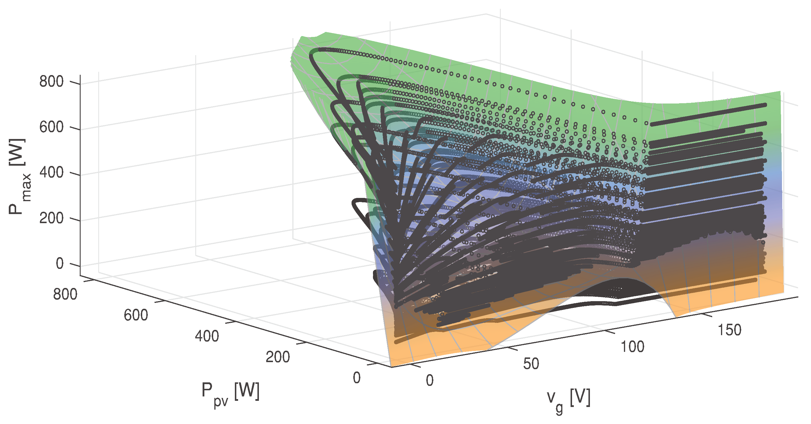
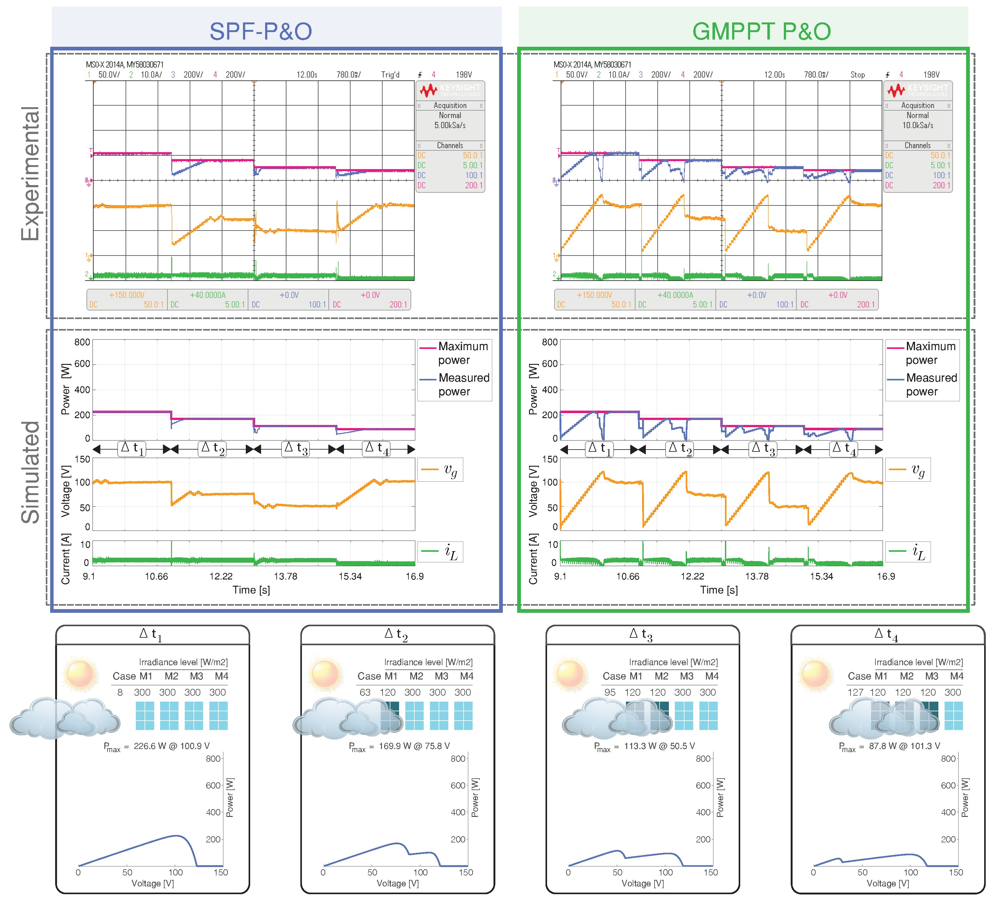
• The proposed SPF-P&O MPPT method is compared with the GMPPT P&O [13], obtaining results that prove a fast convergence and minimum steady-state oscillations for the PV system under 133 different cases of shading patterns.
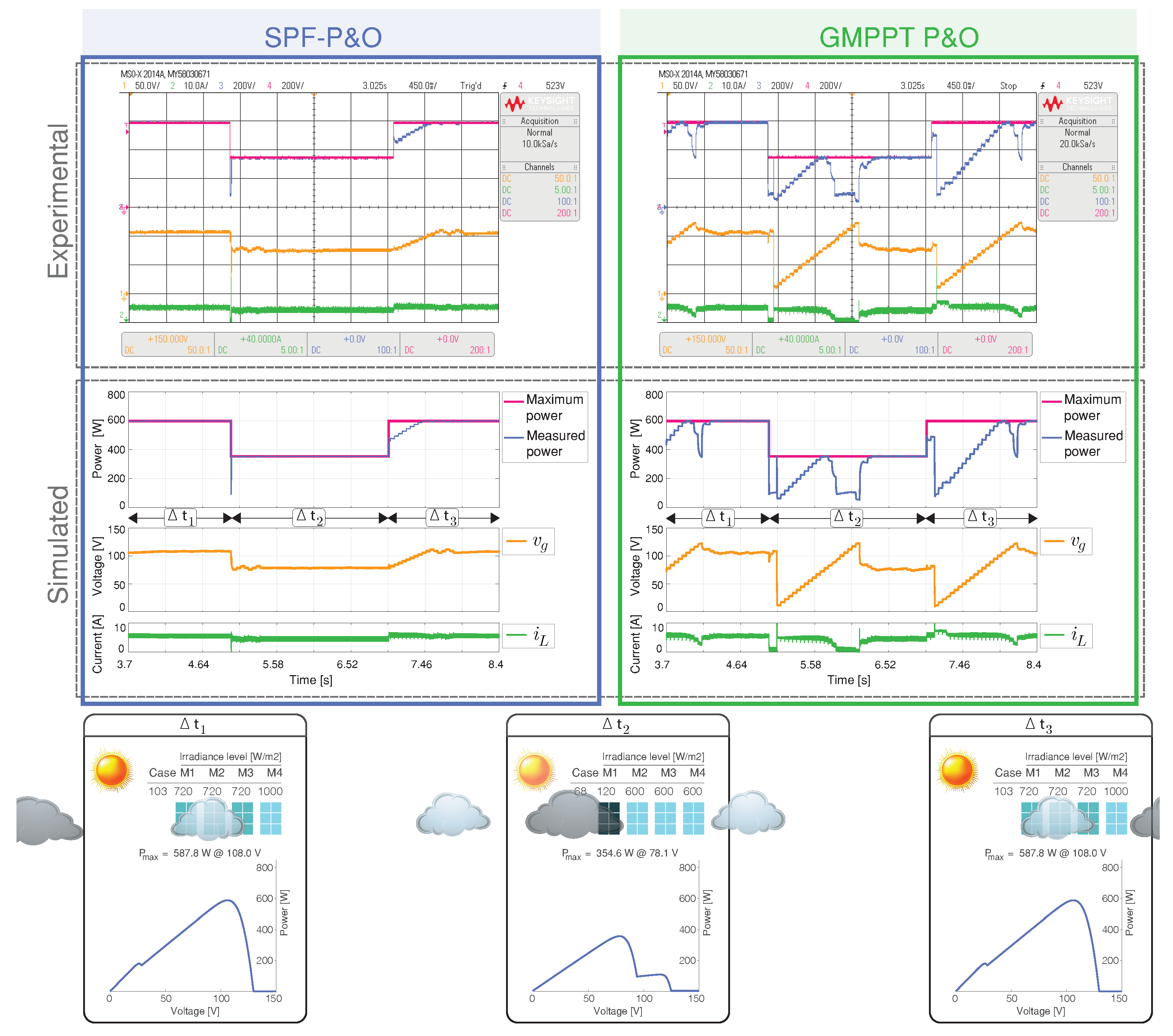
• For the validation of the proposed GMPPT algorithm, six scenarios with different transient of shading patterns are presented: (i) system start-up, (ii) uniform irradiance variations, (iii) sharp change of the (PSCs), (iv) multiple peaks in the P-V characteristic, (v) dark cloud passing, and vi) light cloud passing.
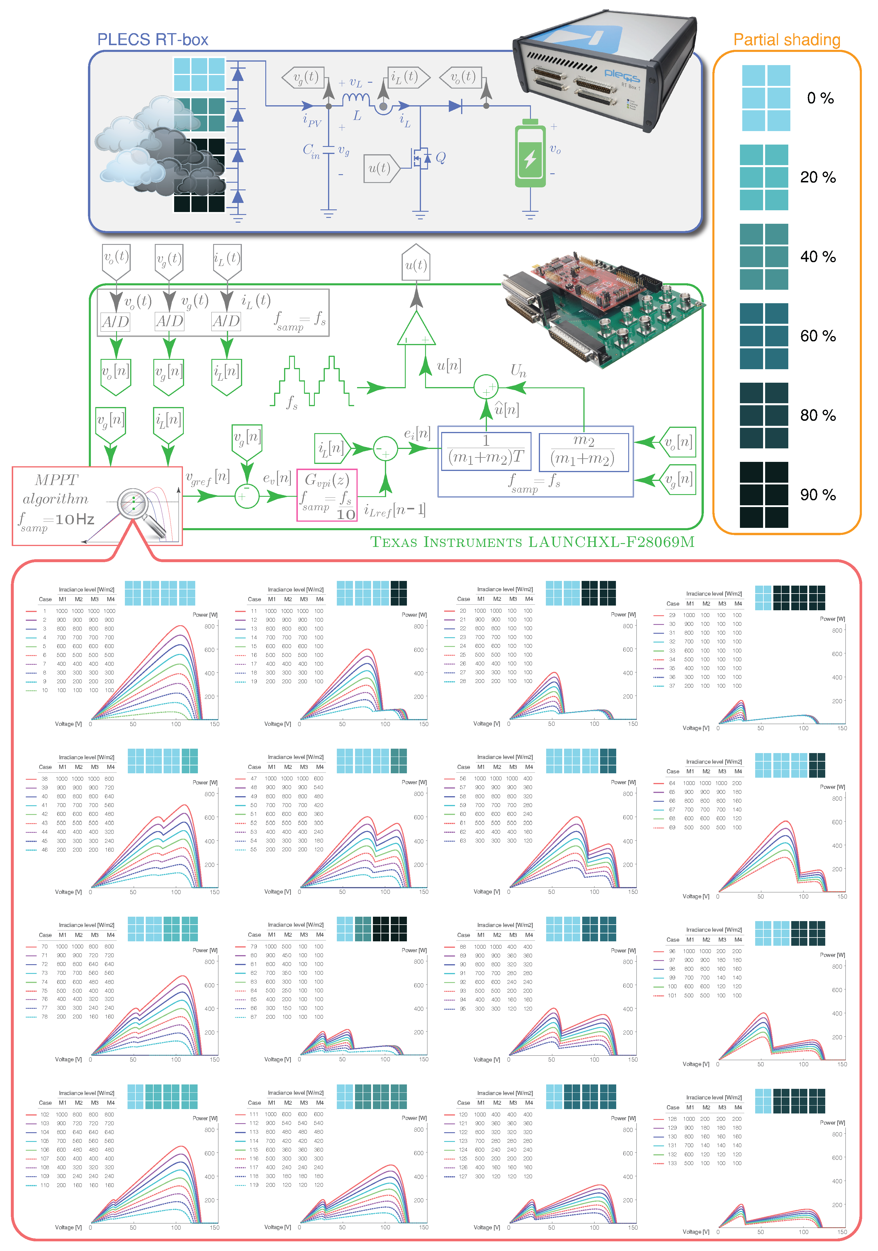
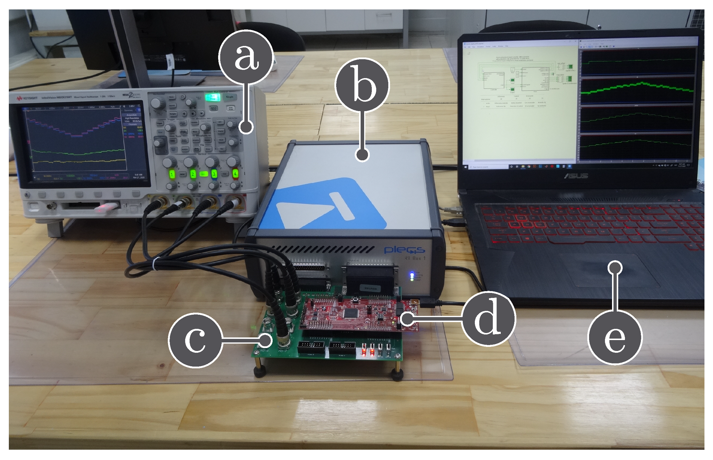
• A two-stage strategy for the experimental PV system is proposed: (i) Modeling the PV array with the DC-DC boost converter using a real-time and high-speed simulator (PLECS RT Box), (ii) Implementing the proposed GMPPT algorithm and the double-loop controller of the DC-DC boost converter in a commercial low-priced digital signal controller (DSC).
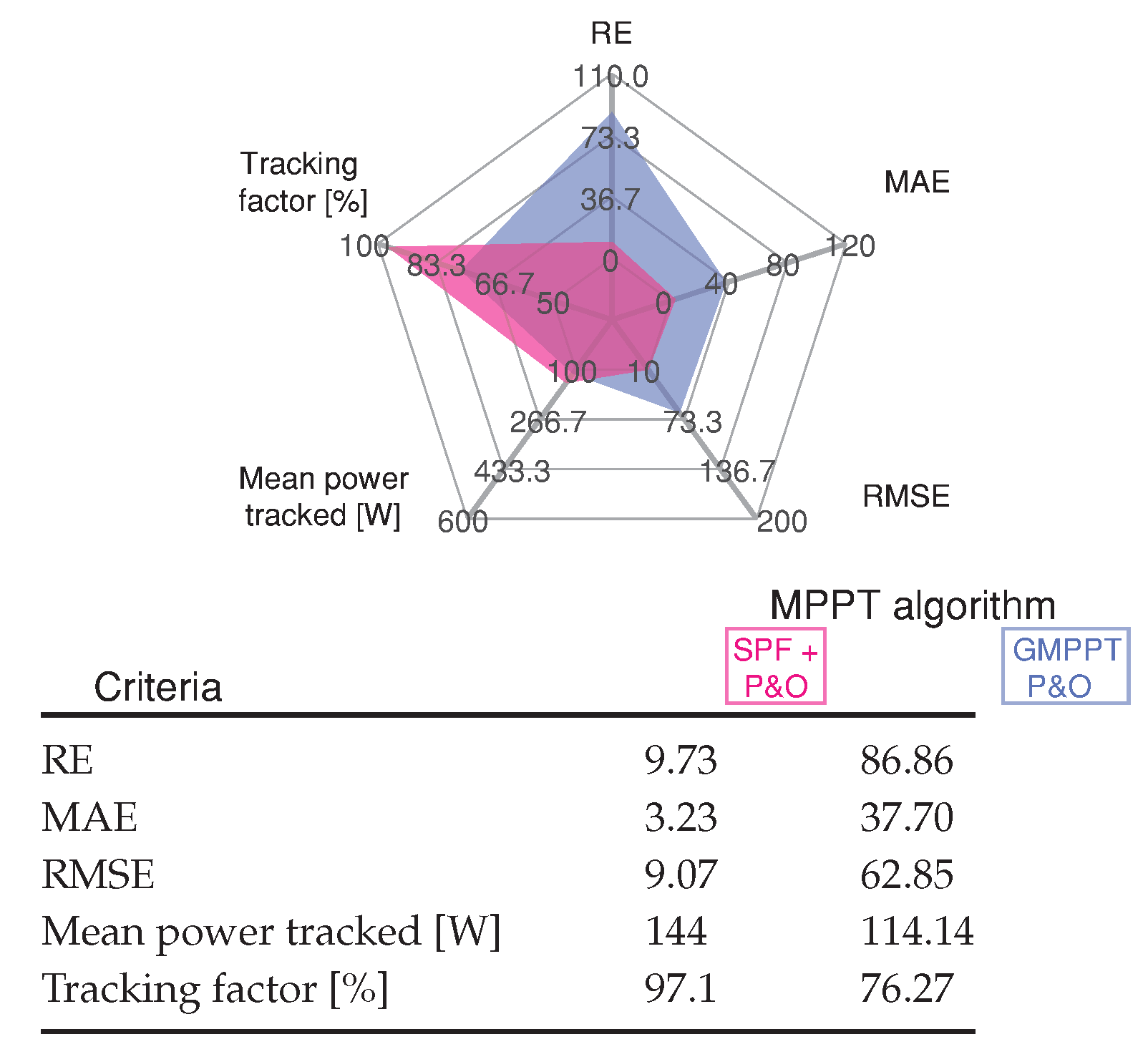
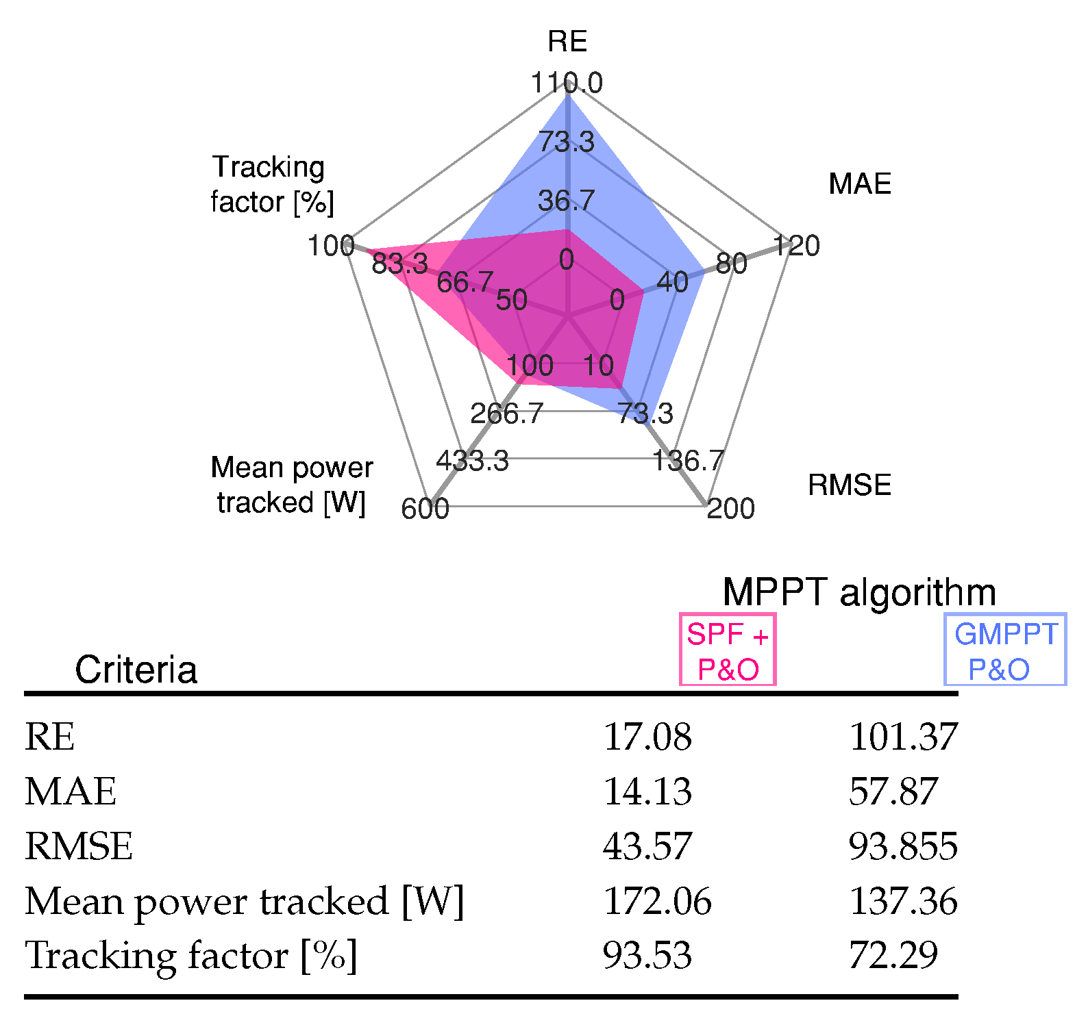
• The simulated and hardware-in-the-loop results of the six scenarios are evaluated using the standard errors, and the mean power tracked and tracking factor scores.
• A nested control loop design is proposed to regulate—along with the SPF-P&O MPPT algorithm—the output voltage of the PV system under challenging environmental conditions. The double-loop control scheme consists of a current (inner-loop) controller and a voltage (outer loop) controller. Low steady-state error under demanding tests including irradiance variations, dynamic partial shading changes and system start-up, and the fast-tracking of control set points, are ensured by each proposed controller. In addition, the implementation of these loops guarantees an independent and fast dynamic response from the system.

The rest of this paper is structured as follows. First, Section 2 shows the PV system and its controllers. Then, the proposed SPF-P&O GMPPT algorithm is explained in Section 3. Next, the numerical simulations and Real-Time HIL Results are detailed in Section 4. Lastly, conclusions and future work are presented in Section 5.

2. PV Modeling

Through a setup of four PV modules, with its respective parallel bypass diodes and all connected in series, the essence of PV string characteristics is studied as shown in Figure 1. This PV string employs a DC-DC boost switching converter to charge a battery while a nested control loop tracks the MPP of the PV system.

Figure 1 depicts the MPPT algorithm and the double-loop controls. Using PLECS, the PV units are modeled as an array of four series-connected KC200GT solar modules whose electrical characteristics are presented in

Table 1. Electrical characteristics of PV module KC200GT.

Electrical Parameters		Value
Maximum power $P_{max}$		200.0 W
Voltage at maximum power $V_{mp}$		26.3 V
Current at maximum power $I_{mp}$		7.61 A
Short-circuit current $I_{sc}$		8.21 A
Open-circuit voltage $V_{oc}$		32.9 V
Temperature coefficient of short-circuit current		$3.18\times {10}^{-1}$ A/${}^{\circ }$C
Temperature coefficient		$-1.23\times {10}^{-1}$ V/${}^{\circ }$C

. Likewise, Figure 1 details the non-linear P-V characteristic for 133 different cases of shading patterns. There are 24 possible permutations for each of the 133 cases, totaling 3192 possible PSCs. Thus, the PV system can be studied under uniform irradiance levels (cases 1 to 10) with a unique peak in the P-V characteristic corresponding to the GMPP. On the other hand, different combinations of PSCs generate multiple peaks in the P-V characteristic, from two to three. Figure 1 shows the nonuniform irradiance levels on the PV modules that produce these PSCs. The GMPP moves with respect to the LMPPs at the multiple P-V characteristic peaks to test different situations with the MPPT algorithms.

The following are the differential equations for the boost converter [17,18,19]:

$${\displaystyle \frac{d{i}_L\left(t\right)}{dt}}={\displaystyle \frac{v_g-(1-u)v_o}{L}}$$

(1)

$${\displaystyle \frac{d{v}_o\left(t\right)}{dt}}={\displaystyle \frac{-v_o}{R_{L}C}}+{\displaystyle \frac{(1-u)i_L}{C}},$$

(2)

where $v_o$ is the output voltage, u represents the control variable $\in \left\{0,1\right\}$ and $i_L$ is the inductor current. For the boost converter, the duty cycle is [17,18,19]:

$$\overline{u}=1-{\displaystyle \frac{{\overline{v}}_g}{{\overline{v}}_o}}.$$

(3)

2.1. Discrete-Time Sliding-Mode Current Control

Designing the inner-loop control for the DC-DC boost converter is complex due to the inherent non-linearity of the converter. Thus, a robust sliding-mode controller is used in this study. This section outlines the discrete-time sliding-mode current control (DSMCC) strategy with a fixed frequency. In order to ensure that the control surface (4) is reached in the next sampling period ($f_{samp}=f_s$), this approach computes the variable control $u\left[n\right]$ in the n-th time sample period. This control has been implemented for switching systems in [20,21,22].

$$s\left[n\right]=i_{Lref}[n-1]-i_L\left[n\right].$$

(4)

Equation (2) is used to calculate the inductor current slopes of the boost converter, presented in

Table 2. Slope of the inductor current waveform.

Converter		${\mathit{m}}_1$		$-{\mathit{m}}_2$
Boost		${\displaystyle \frac{v_g}{L}}$		${\displaystyle \frac{v_g-v_o}{L}}$

. Assuming the averaged model of the inductor current slope of the converter $\frac{d{i}_L}{dt}\approx \frac{i_L[n+1]-i_L\left[n\right]}{T}$, the Euler approximation heads to the next discrete-time inductor current expression:

$$i_L[n+1]=i_L\left[n\right]+T(m_1+m_2)u\left[n\right]-m_{2}T$$

(5)

being T the sampling or switching period. Consequently, the resulting duty cycle expression is:

$$u\left[n\right]=\frac{1}{(m_1+m_2)T}e\left[n\right]+\frac{m_2}{m_1+m_2},$$

(6)

where $e\left[n\right]=i_{Lref}\left[n\right]-i_L\left[n\right]$, being $i_{Lref}\left[n\right]=i_L[n+1]$ (see Figure 1). Using the expressions for $m_1$ and $-m_2$ for the output current slopes from Table 2 in (6), the boost converter’s control law is given by:

$$u\left[n\right]=\frac{L}{v_o\left[n\right]T}e\left[n\right]+1-\frac{v_g\left[n\right]}{v_o\left[n\right]}.$$

(7)

2.2. Discrete-Time PI Voltage Control

The input voltage of the boost converter $v_g$ is regulated for the external loop using a proportional-integrator controller. The forward Euler method is used to express the controller transfer function in the z domain as follows:

$$G_{vpi}\left(z\right)=K_{pv}+\frac{K_{iv}{T}_{samp}}{z-1},$$

(8)

where $T_{samp}=1/f_{samp}$,

$$K_{pv}=2\mathrm{\pi }{C}_{in}{\mathit{f}}_c,$$

(9)

and

$$K_{iv}=\frac{K_{pv}}{T_i},$$

(10)

with $C_{in}$ representing the input capacitor. For the voltage loop ($f_c$), the crossover frequency (CF) value should be lower than the current loop CF. Furthermore, the PI zero should be below $f_c$ ($1/\left(2\mathrm{\pi }{T}_i\right)<f_c$).

3. SPF-P&O MPPT

3.1. Maximum Power Point Tracking (MPPT) Algorithm

The Maximum Power Point Tracking (MPPT) control keeps the power transfer at the highest efficiency, optimizing the PV system performance in any radiation and temperature conditions that the solar panels undergo. The MPPT approach allows the PV module to function at its maximum power point by controlling the switching converter [23]. This section briefly explains the “Perturb and Observe” benchmark method before introducing the offered MPPT method.

3.2. Conventional “Perturb and Observe” Method

The so-called “Perturb and Observe” (P&O) method is widely used due to its simplicity and low cost [24,25,26]. This algorithm provokes perturbations by either decreasing or increasing the reference voltage according to the output power PV module. If the current measured power $P\left[n\right]$ is higher than its previous sampled value $P[n-1]$, the voltage change continues in the same direction. Otherwise, it is reversed. Next, the PV module voltage is compared to the maximum voltage, to predict the MPP. Finally, a power step of the PV module [24] is produced through a small step of reference voltage. The P&O-based MPPT is abbreviated as MPPT-P&O.

3.3. Proposed MPPT Method

This work proposes a polynomial curve-fitting approach in favor of a more accurate MPP estimation. This approach, known as Surface-based Polynomial Fitting (MPPT-SPF), works as explained below:

3.3.1. Curve-Based Fitting

The fundamentals of a polynomial model ($y=f\left(x\right)$) for any curve can be expressed in mathematical terms as follows:

$$y\left\{{\rho }_N\right\}=\sum _{i=1}^{N+1}{C}_i{x}^{N+1-i},$$

(11)

where x is the input times series, $y\left\{{\rho }_N\right\}$ is the output time series, n is the degree of the polynomial, such that $1\le N\le 9$, and $N+1$ is the order of the polynomial. In this case, the order is the number of coefficients to be adjusted, while the degree represents the highest power of the predictor variable.

Below, and based on their degree, polynomials are presented. For example, a four-degree polynomial is given by:

$$y\left\{{\rho }_4\right\}=f\left(x\right)=C_1{x}^4+C_2{x}^3+C_3{x}^2+C_{4}x+C_5.$$

(12)

Polynomials are helpful when a simple empirical model is needed. Hence, a polynomial model is suitable for interpolation and extrapolation processes or characterizing data using a global fit.

Polynomial fitting is reasonably flexible when dealing with simple data structures. However, fitting can become unstable for high-degree polynomials. Moreover, although all polynomials fit correctly within a predefined data range, they diverge significantly outside of it.

Curve-fitting with high-degree polynomials can result in scale affectations because it uses predictor values as the basis for a matrix with high values. This problem can be addressed by preprocessing input data using z-score normalization, i.e., centering to zero mean and scaling to unit standard deviation [16].

3.3.2. Surface-Based Fitting

The output time series is represented as $z=f(x,y)$ when the fitting $f(·)$ involves two input time series. For MPPT purposes, the variables are defined as follows:

• z: maximum power estimation for PV module current and voltage measurements ($P_{max}$),
• x: current $i_L\left[n\right]$,
• y: power measurement from the PV module $P_{pv}\left[n\right]$.

The following notation is used for polynomial surfaces: ${\rho }_{ij}$ is the fitting type, where j represents the degree of y and, on the other hand, i the degree of x. Additionally, the maximum value for i and for j [27] is 5. The maximum between i and j is the overall degree of the polynomial. The degree of x is going to be less than or equal to i in each term. Likewise, in each term, the degree of y is going to be less than or equal to j. Accordingly, a surface with i and j degrees is denoted as $z\left\{{\rho }_{ij}\right\}=f(x,y)$. Some examples are mentioned in

Table 3. Examples of polynomial models for surfaces.

Polynomial Models	Equations
${\rho }_{21}$	$z\left[{\rho }_{21}\right]=C_{00}+C_{10}x+C_{01}y+C_{20}{x}^2+C_{11}xy$
${\rho }_{13}$	$z\left[{\rho }_{13}\right]=C_{00}+C_{10}x+C_{01}y+C_{11}xy+C_{02}{y}^2+C_{12}x{y}^2+C_{03}{y}^3$
${\rho }_{55}$	$z\left[{\rho }_{55}\right]=C_{00}+C_{10}x+C_{01}y+\dots +C_{14}x{y}^4+C_{05}{y}^5$

.

Table 4. Polynomial model terms.

Degree of Term		0		1		2		3		4
0		1		y		$y^2$		$y^3$		$y^4$
1		x		$xy$		$x{y}^2$		$x{y}^3$		$x{y}^4$
2		$x^2$		$x^{2}y$		$x^2{y}^2$		$x^2{y}^3$		-
3		$x^3$		$x^{3}y$		$x^3{y}^2$		-		-
4		$x^4$		$x^{4}y$		-		-		-
5		$x^5$		-		-		-		-

shows the degrees that make up the model terms. For example, for an x degree of 1 and a y degree of 3, the name of the model will be ${\rho }_{13}$. The mathematical foundation of the numerical curve-fitting methods is further detailed in [16].

A function is obtained from the ${\rho }_{ij}$ approach that precisely fits the behavior and general trend of the analyzed data. Next, the most accurate fitting is found, considering both the criteria to quantify the adjusting procedure suitability and the polynomial to be tuned to represent the input data. The relationship between the obtained polynomial degree, the curve adjustment, and the values to interpolate is obtained from this adjustment. Finally, a five-degree polynomial is generated from a given data sequence in the form $\left(x\right[n],y[n\left]\right)$, as shown below:

$$\begin{array}{cc}\hfill f(x,y)=& C_{00}+C_{10}x+C_{01}y+C_{20}{x}^2+C_{11}xy\hfill \\ \hfill & +C_{02}{y}^2+C_{30}{x}^3+C_{21}{x}^{2}y+C_{12}x{y}^2+C_{03}{y}^3\hfill \\ \hfill & +C_{40}{x}^4+C_{31}{x}^{3}y+C_{22}{x}^2{y}^2+C_{13}x{y}^3+C_{04}{y}^4\hfill \\ \hfill & +C_{50}{x}^5+C_{41}{x}^{4}y+C_{32}{x}^3{y}^2+C_{23}{x}^2{y}^3+C_{14}x{y}^4.\hfill \end{array}$$

(13)

The afore-developed analysis allows assessing how well the curve fits the data. Goodness-of-fit is measured by determining the accuracy of the coefficients based on the 95% confidence limits. The polynomial coefficients determined from the robust fitting of the data are:

$$\begin{array}{cc}\hfill & C_{00}=186.8(184.7,188.9),\hfill \\ \hfill & C_{10}=-14.14(-14.55,-13.73),\hfill \\ \hfill & C_{01}=6.969(6.883,7.056),\hfill \\ \hfill & C_{20}=0.3872(0.3721,0.4022),\hfill \\ \hfill & C_{11}=-0.3113(-0.316,-0.3065),\hfill \\ \hfill & C_{02}=0.009194(0.008359,0.01003),\hfill \\ \hfill & C_{30}=-0.004332(-0.004533,-0.00413),\hfill \\ \hfill & C_{21}=0.006992(0.006861,0.007124),\hfill \\ \hfill & C_{12}=-0.0004896(-0.0005158,-0.0004635),\hfill \\ \hfill & C_{03}=7.545e-06(4.966e-06,1.012e-05),\hfill \\ \hfill & C_{40}=2.297e-05(2.184e-05,2.409e-05),\hfill \\ \hfill & C_{31}=-7.728e-05(-7.875e-05,-7.581e-05),\hfill \\ \hfill & C_{22}=1.026e-05(9.913e-06,1.061e-05),\hfill \\ \hfill & C_{13}=-6.762e-07(-7.171e-07,-6.353e-07),\hfill \\ \hfill & C_{04}=2.86e-08(2.565e-08,3.155e-08),\hfill \\ \hfill & C_{50}=-4.633e-08(-4.858e-08,-4.407e-08),\hfill \\ \hfill & C_{41}=3.104e-07(3.049e-07,3.158e-07),\hfill \\ \hfill & C_{32}=-5.768e-08(-5.93e-08,-5.607e-08),\hfill \\ \hfill & C_{23}=5.3e-09(5.014e-09,5.586e-09),\mathrm{and}\hfill \\ \hfill & C_{14}=-2.523e-10(-2.799e-10,-2.248e-10).\hfill \end{array}$$

generating the following polynomial:

$$\begin{array}{cc}\hfill f(x,y)=& 186.8-14.14x+6.969y+0.3872x^2-0.3113xy\hfill \\ \hfill & +0.009194y^2-0.004332x^3+0.006992x^{2}y-0.0004896x{y}^2\hfill \\ \hfill & +7.545e-06y^3+2.297e-05x^4-7.728e-05x^{3}y\hfill \\ \hfill & +1.026e-05x^2{y}^2-6.762e-07x{y}^3+2.86e-08y^4\hfill \\ \hfill & -4.633e-08x^5+3.104e-07x^{4}y-5.768e-08x^3{y}^2\hfill \\ \hfill & +5.3e-09x^2{y}^3-2.523e-10x{y}^4.\hfill \end{array}$$

(14)

As a result, the obtained fitting reaches a remarkable $0.9507$ R-square, indicating a significant data trend and a good model fitting. Moreover, a $38.74$ root mean square error (RMSE) and a $9.477e+07$ sum of square error (SSE) estimation are reached. Figure 2 depicts the previous adjustment as a MPP surface in terms of $P_{pv}$ and $v_g$.

Validation and implementation of the MPPT-SPF aim to maximize the available energy of the connected solar modules at any given moment during operation. Hence, MPPT continually samples the output of the PV cells and adjusts the voltage and current so that the PV system generates maximum power regardless of environmental conditions.

Additionally, by following the approach described in [28], uncertainty values for all the coefficients can be calculated. To do so, consider the vector $\mathbf{C}$ holding the estimates of the coefficients given by:

$$\begin{array}{c}\hfill \tilde{\mathbf{C}}={\left({\mathbf{\Phi }}^{\top }\mathbf{\Phi }\right)}^{-1}{\mathbf{\Phi }}^{\top }\mathbf{E},\end{array}$$

(15)

where

$$\mathbf{\Phi }=[{\mathbf{1}}_m,\mathbf{x},\mathbf{y},{\mathbf{x}}^{\mathbf{2}},\mathbf{xy},{\mathbf{y}}^{\mathbf{2}},{\mathbf{x}}^{\mathbf{3}},{\mathbf{x}}^{\mathbf{2}}\mathbf{y},{\mathbf{xy}}^{\mathbf{2}},{\mathbf{y}}^{\mathbf{3}},{\mathbf{x}}^{\mathbf{4}},{\mathbf{x}}^{\mathbf{3}}\mathbf{y},{\mathbf{x}}^{\mathbf{2}}{\mathbf{y}}^{\mathbf{2}},{\mathbf{xy}}^{\mathbf{3}},{\mathbf{y}}^{\mathbf{4}},{\mathbf{x}}^{\mathbf{5}}{\mathbf{x}}^{\mathbf{4}}\mathbf{y},{\mathbf{x}}^{\mathbf{3}}{\mathbf{y}}^{\mathbf{2}},{\mathbf{x}}^{\mathbf{2}}{\mathbf{y}}^{\mathbf{3}},{\mathbf{xy}}^{\mathbf{4}}],$$

(16)

and

$$\mathbf{E}=[{\epsilon }_1,\dots ,{\epsilon }_m],$$

(17)

with m denoting the number of samples, $varepsilo{n}_i$ being the error of approximation and $i\in \{1,\dots ,m\}$. Then, the uncertainty $u\left(C_j\right)$ for the coefficient j can be estimated as:

$$\begin{array}{c}\hfill u\left(C_j\right)=\sqrt{{\displaystyle \frac{{\left(\mathbf{\Phi }\tilde{\mathbf{C}}-\mathbf{E}\right)}^{\top }\left(\mathbf{\Phi }\tilde{\mathbf{C}}-\mathbf{E}\right)}{m-3}}}\sqrt{{\theta }_{jj}},\end{array}$$

(18)

where

$$\begin{array}{c}\hfill \mathbf{\Theta }={\left({\mathbf{\Phi }}^{\top }\mathbf{\Phi }\right)}^{-1},\end{array}$$

(19)

${\theta }_{jj}$ is the entry $jj$ of matrix $\mathbf{\Theta }$ and $j\in \{1,\dots ,20\}$. In this case, all the uncertainty values are admissible as can be noted in the following:

$$\begin{array}{cc}\hfill & u\left(C_1\right)=u\left(C_{00}\right)=-8.92\times {10}^{11},\hfill \\ \hfill & u\left(C_2\right)=u\left(C_{10}\right)=-4.09\times {10}^9,\hfill \\ \hfill & u\left(C_3\right)=u\left(C_{01}\right)=2.49\times {10}^5,\hfill \\ \hfill & u\left(C_4\right)=u\left(C_{20}\right)=-2.79\times {10}^6,\hfill \\ \hfill & u\left(C_5\right)=u\left(C_{11}\right)=7.36\times {10}^3,\hfill \\ \hfill & u\left(C_6\right)=u\left(C_{02}\right)=3.61\times {10}^1,\hfill \\ \hfill & u\left(C_7\right)=u\left(C_{30}\right)=-4.53\times {10}^2,\hfill \\ \hfill & u\left(C_8\right)=u\left(C_{21}\right)=4.33,\hfill \\ \hfill & u\left(C_9\right)=u\left(C_{12}\right)=2.5\times {10}^{-2},\hfill \\ \hfill & u\left(C_{10}\right)=u\left(C_{03}\right)=1.09\times {10}^{-4},\hfill \\ \hfill & u\left(C_{11}\right)=u\left(C_{40}\right)=-1.75\times {10}^{-2},\hfill \\ \hfill & u\left(C_{12}\right)=u\left(C_{31}\right)=3.77\times {10}^{-4},\hfill \\ \hfill & u\left(C_{13}\right)=u\left(C_{22}\right)=2.13\times {10}^{-06},\hfill \\ \hfill & u\left(C_{14}\right)=u\left(C_{13}\right)=5.14\times {10}^{-08},\hfill \\ \hfill & u\left(C_{15}\right)=u\left(C_{04}\right)=4.55\times {10}^{-12},\hfill \\ \hfill & u\left(C_{16}\right)=u\left(C_{50}\right)=-1.05\times {10}^{-07},\hfill \\ \hfill & u\left(C_{17}\right)=u\left(C_{41}\right)=4.06\times {10}^{-09},\hfill \\ \hfill & u\left(C_{18}\right)=u\left(C_{32}\right)=2.55\times {10}^{-11},\hfill \\ \hfill & u\left(C_{19}\right)=u\left(C_{23}\right)=1.52\times {10}^{-12},\mathrm{and}\hfill \\ \hfill & u\left(C_{20}\right)=u\left(C_{14}\right)=5.12\times {10}^{-16}.\hfill \end{array}$$

3.4. SPF-P&O Algorithm

The SPF-P&O GMPPT algorithm is detailed in Algorithm 1, which works as follows: Its objective is to obtain the input voltage reference ($v_{gref}$) for the boost converter from the measurement of the output voltage and output current of the PV module array. In this way, the maximum power characteristic ($P_{max}$) associated with the measured of current and voltage is obtaining from the expression (14). Once $P_{max}$ is estimated, the voltage reference for the P&O is selected by searching from a register of possible solutions for power point maximum power ($P_{mpp}$).

When power changes, greater than or equal to reference $\Delta P_{pv}[\%]$ occur, the MPPT-SPF algorithm is executed, so:

$$\frac{\left|P_{pvnew}-P_{pvlast}\right|}{P_{pvlast}}\ge \Delta P_{pv}[\%],$$

(20)

where $P_{pvnew}$ is the actual power measurement and $P_{pvlast}$ is the previous power measurement.

The GMPP search will again execute if the condition (20) is satisfied. This condition ensures that the expression (14) is evaluated to detect the optimal voltage solution for the GMPP even if there is any change in solar irradiance.

Algorithm 1: SPF-P&O GMPPT algorithm running at the microcontroller (see Figure 1).

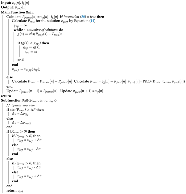
4. Simulation and Real-Time HIL Results

In this section, the SPF-P&O MPPT algorithm is validated using a DC-DC boost converter through hardware in the loop (HIL). PLECS RT Box 1 implements the stage power converter and the PV array, and 6.6 $\mathsf{\mu }$s is the sampled time to model the converter. And the values of the boost converter components are: $C_{in}=200\mathsf{\mu }$F, $L=1$mH, $V_o=160$ V and $f_s=25$ kHz. Through the TI 28069M LaunchPad, which is a low-cost Texas Instrument microcontroller, different controls that integrate the PV global system control scheme are implemented as presented Figure 1. Figure 3 shows the setup for HIL experiments.

The proposed SPF-P&O MPPT method is compared with a GMPPT P&O algorithm studied in [13], which realizes a voltage swept in partial shading conditions across the entire voltage range (from 0 to the open voltage value) for the PV system. The voltage reference that produces the maximum power is used to initialize after the voltage swept the P&O algorithm.

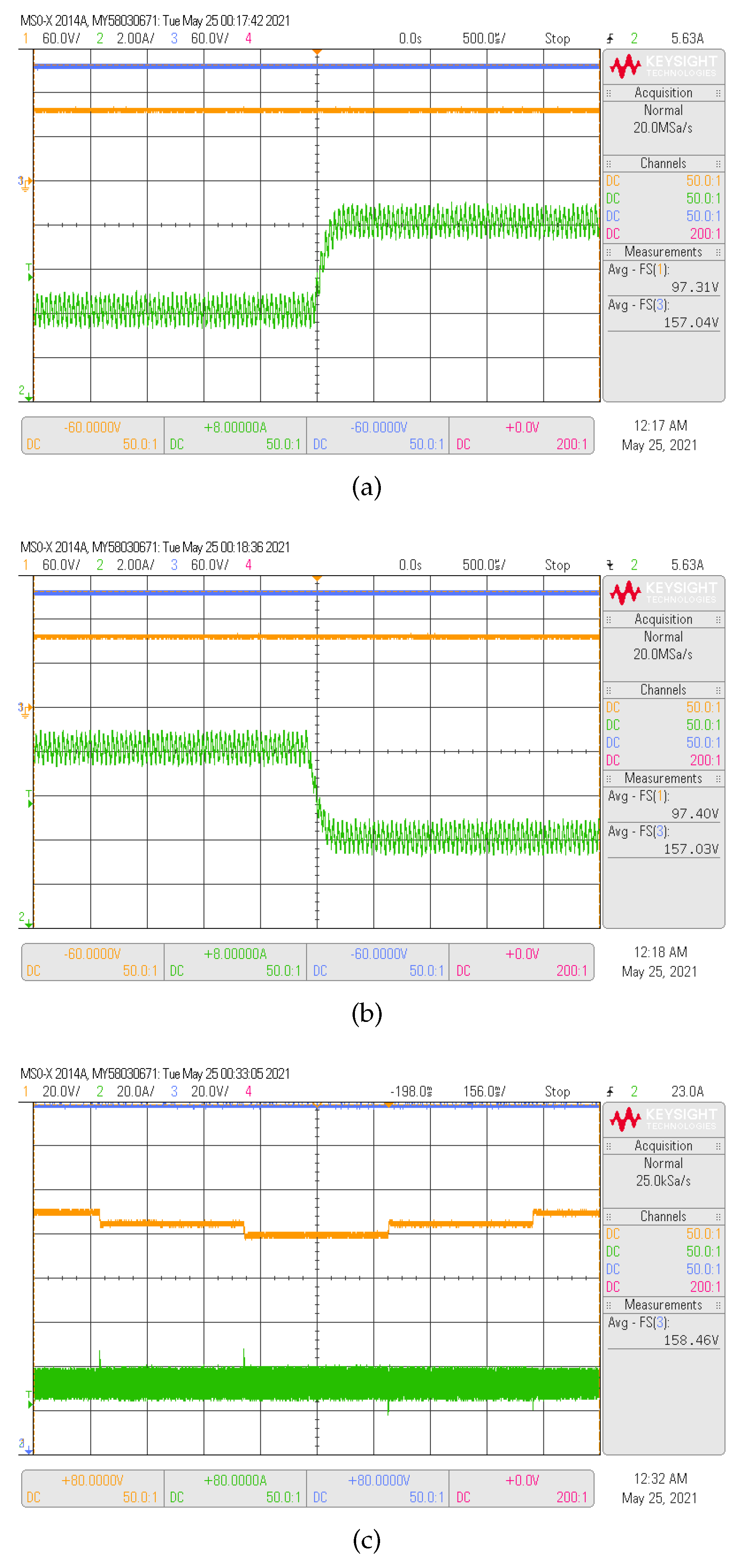
4.1. Inner-Loop Current Control Results

Figure 4 illustrates the transient responses for the inductor current of the boost converter in reaction to variations of the current reference. Where $v_g$, $v_o$ and $i_L$ are the signals sampled for the control, and 500 $\mathsf{\mu }$s is the sampling time. The current reference is changed from 4 A to 8 A and back to 4 A, as can be observed in Figure 4a,b. to ensure a boost operation, the output voltage is $V_o=160$ V and the input voltage is set in 100 V. Smooth transitions during reference changes are found, settling times near 250 $\mathsf{\mu }$s and no overshoot. As shown, the inductor current is well regulated. The inductor currents followed the change in the current reference perfectly. During the current step reference change, the current control performance is validated.

4.2. Double-Loop Results

To demonstrate the effectiveness of the external loop control, voltage reference variations from 100 V to 110 V with a step between variations of 5 V for external loop validation, are presented in Figure 4c. The crossover frequency (CF) corresponds to $f_c=500$ Hz, allowing the proportional gain calculation according to (9). Since the location of the PI zero in Equation (10) is lower than $f_c$ ($1/\left(2\mathrm{\pi }{T}_i\right)<{\mathit{f}}_c$), $T_i=3.18e-3$ s was chosen.

Every 400 $\mathsf{\mu }$s, the voltage regulator ($G_{vpi}\left(z\right)$) calculates the inductor current reference as shown in Figure 1. And current transitions, caused by the voltage changes, are smooth and the voltage reference is concisely tracked as can be appreciated from Figure 4c.

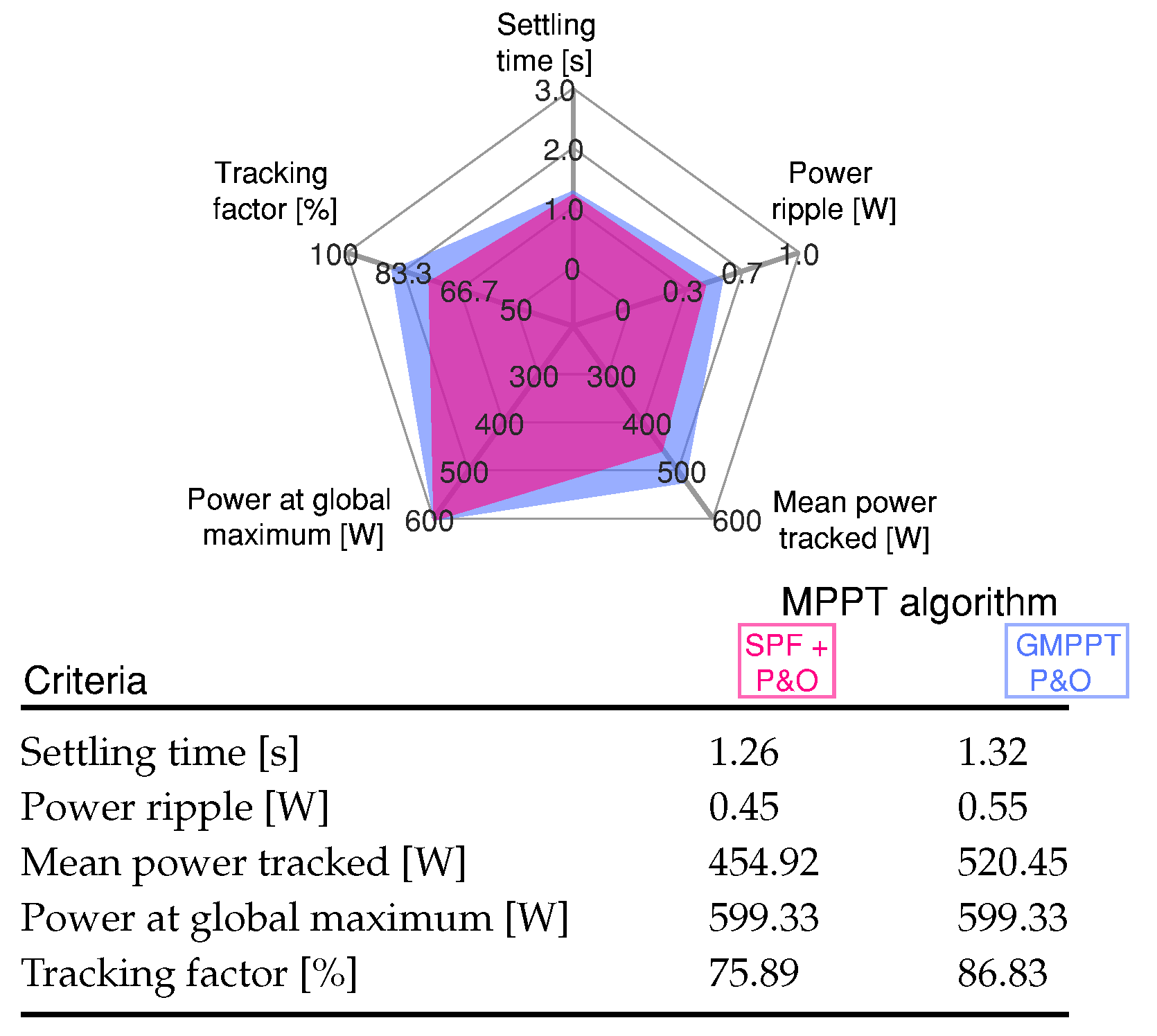
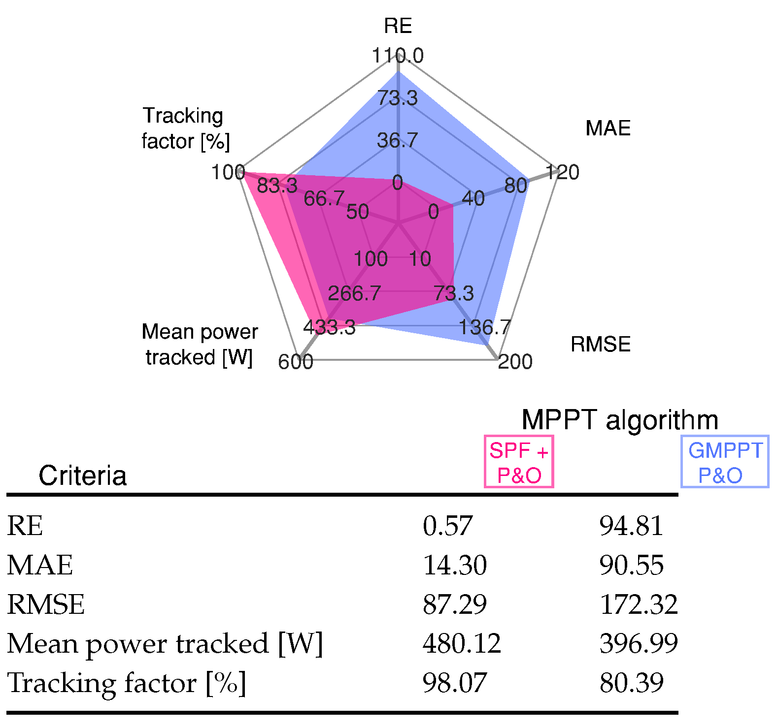
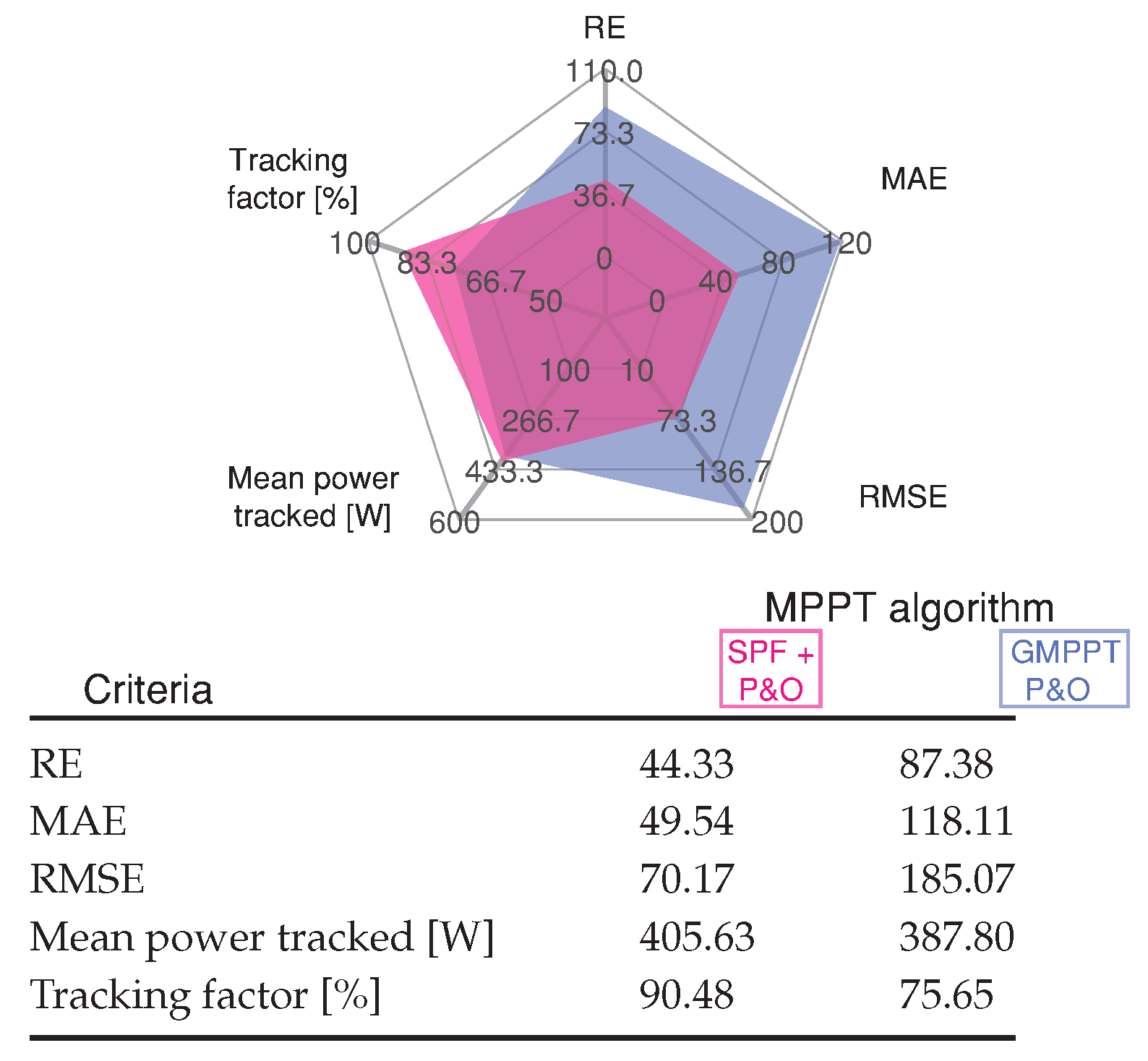
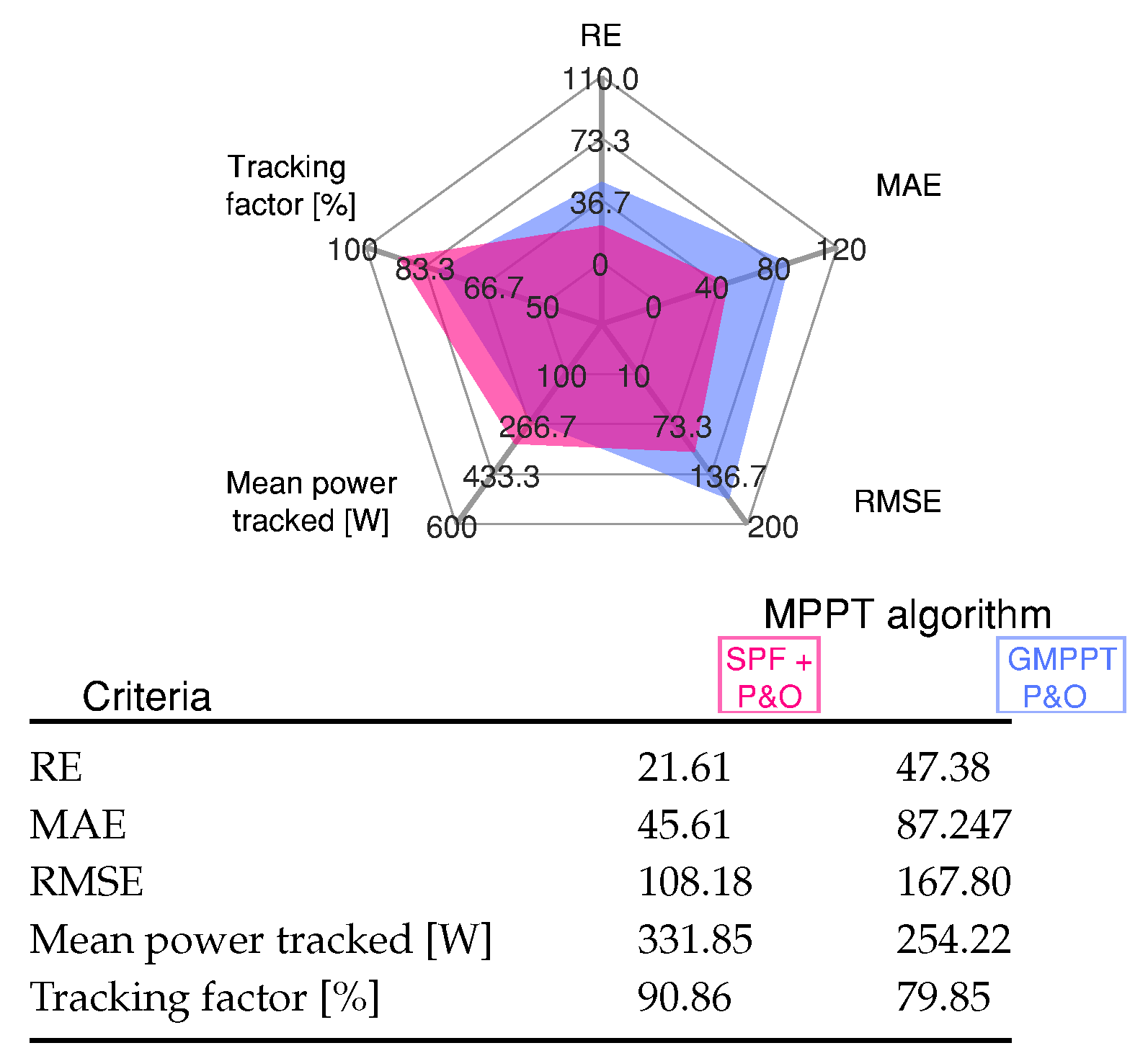
4.3. GMPPT P&O and Proposed SPF-P&O Method Comparison

The proposed method is compared with the GMPPT P&O studied in [13], every 100 ms the GMPPT algorithms are executed to provide a new voltage reference for the voltage loop control, as shown in Figure 1 for the GMPPT algorithm block. For the SPF-P&O, $\Delta P_{pv}[\%]$ from expression (20) is set to 8%. The inner current loop is updating at 25 kHz, the outer voltage loop is calculating at $2.5$ kHz, and the MPPT strategy is computing at 10 Hz, these strategies are implemented in the DSC.

These scale time differences between the systems are challenging but at the same time advantageous to implement an MPPT based on a finite-state machine.

For the validation of the proposed algorithm, six scenarios with different transient of the cases presented in Figure 1 are described below.

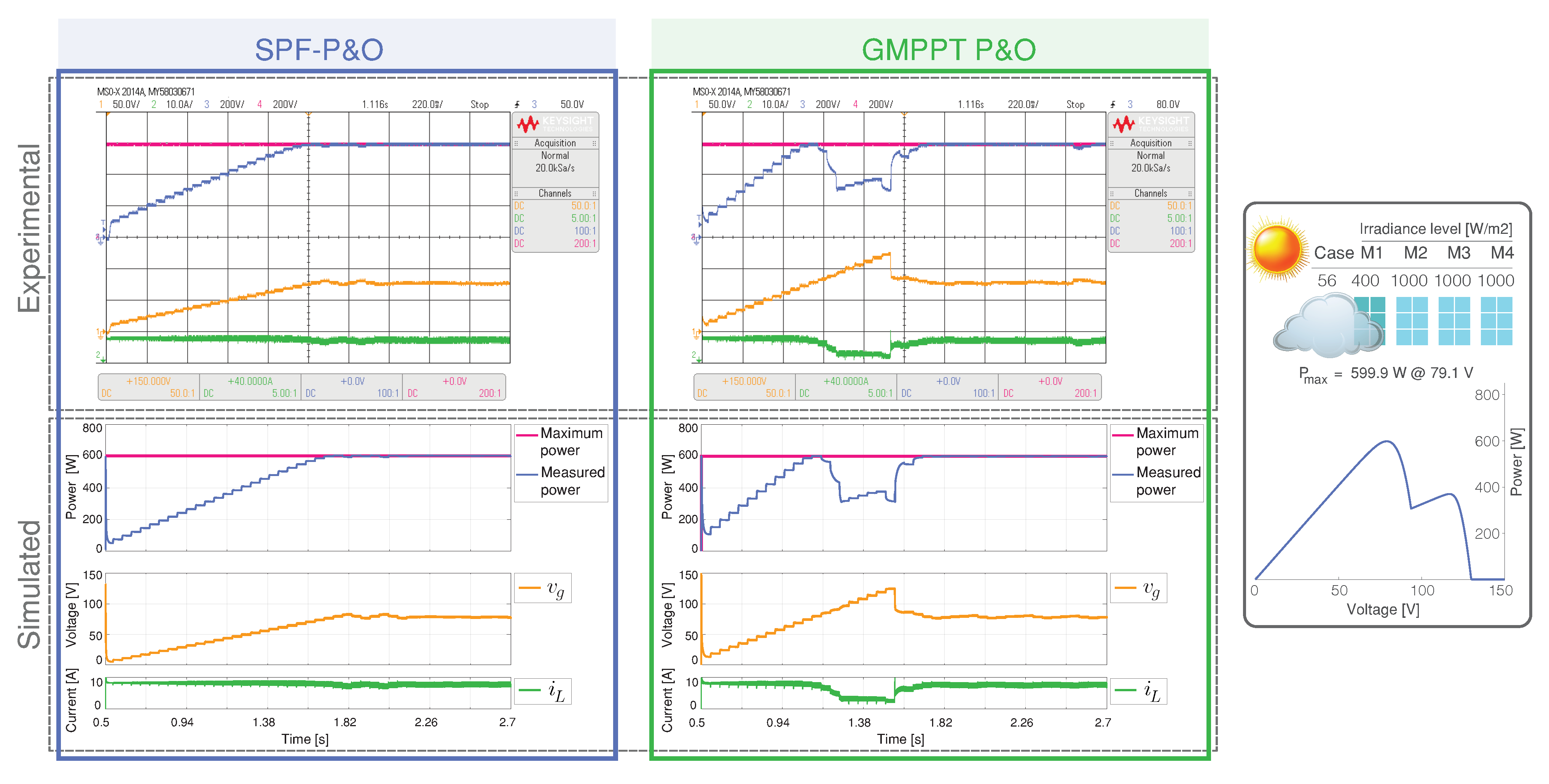
4.3.1. Scenario 1: System Start-Up

This scenario presents the start-up with the panels’ irradiance levels corresponding to case 56 of Figure 1.

Figure 5 shows, corresponding to the maximum power, the transient behavior from zero current until an equilibrium point, where three modules have an irradiance of 1000 W/m${}^2$ and a module of 400 W/m${}^2$.

In Figure 5, both GMPPT algorithms reach the steady-state close to 1.3 s, with the proposed MPPT a uniform step voltage reference to tracking the MPP (599.9 W at 79.1 V) while the system starts up.

The proposed SPF-P&O algorithm works at the optimum point, without oscillation, as is shown in the input voltage signal after it has been tracked. Due to the GMPPT P&O realized a swept of voltage, the reference voltage is increased until 120 V to find the GMPPT at 79.1 V.

In Figure 6, a quantitative analysis can be observed of the proposed GMPPT method and GMPPT P&O method, and the results can be seen in Figure 5. These results confirm a similar performance for both methods through the start-up, where the GMPPT P&O algorithm has a higher tracking factor because the mean power tracked value is closer to the global power maximum.

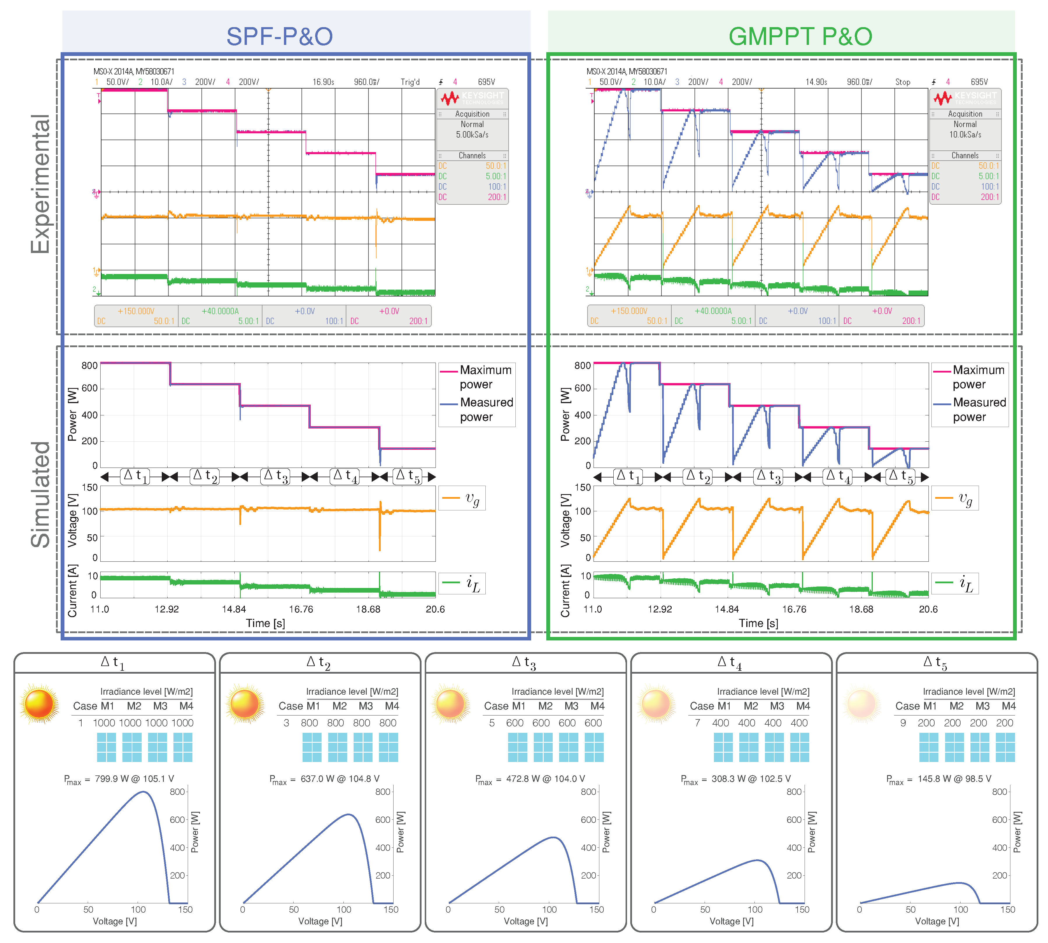
4.3.2. Scenario 2: Uniform Irradiance Variations

Scenario 2 studies the results for the MPPT techniques under uniform irradiance variations as shown in Figure 7. The irradiance sequence corresponds to cases 1, 3, 5, 7, and 9 shown in Figure 1.

The proposed algorithm outputs the optimal voltage reference for the case and tracks the MPP faster while the GMPPT P&O has a slow convergence.

The proposed model facilitates the calculation and estimation of the variable of interest with high levels of accuracy; however, its proper evaluation through the results obtained to ensure its accuracy is crucial. Certainly, this evaluation can be performed by analyzing the errors, such as the mean absolute error (MAE), the relative error (RE) and the root mean square error (RMSE) and evaluate the performance of the results obtained [29,30], whose equations can be written as follows:

$$\mathrm{RE}=\frac{{\sum }_{i=1}^m(P_{pvi}-P_{mpp})}{P_{mpp}}100[\%],$$

(21)

$$\mathrm{MAE}=\frac{{\sum }_{i=1}^m|P_{pvi}-P_{mpp}|}{m},\mathrm{and}$$

(22)

$$\mathrm{RMSE}=\sqrt{\frac{{\sum }_{i=1}^m{(P_{pvi}-P_{mpp})}^2}{m}},$$

(23)

where $P_{pvi}$ represents the measured power of the PV module, $P_{mpp}$ is the available MPP power of the solar module, and m the total number of sampling data. Figure 8 shows the sensitivity of the MPPT algorithms through MAE, RE, and RMSE for the results shown in Figure 7.

Standard error values indicate that the performance of the proposed MPPT algorithm has higher effectiveness in tracking the maximum power point. This statistical analysis shows that the SPF-P&O method reaches the lowest value for the error compared to the GMPPT P&O algorithm. The proposed SPF-P&O algorithm has a tracking factor of 98.07%, while for the GMPPT P&O method, the tracking factor is 80.39%.

4.3.3. Scenario 3: Sharp Change of the PSCs

Scenario 3 presents a sharp change between case 103 and case 68, producing high PV power variations from 588 W to 355 W. Figure 9 shows simulated and HIL results of the GMPP tracking performance. The MPPT tracking efficiency for the GMPPT P&O method is 75.65%, while the 90.48% is achieved by the SPF-P&O proposed method. Figure 10 show the measure of the standard error for each GMPPT method, where the SPF-P&O GMPPT method has minimum error. As can be seen in the input voltage of the converter in Figure 9 and by the inductor current, the PV array always operates in an oscillating mode for the GMPPT P&O method.

Therefore, the proposed GMPPT method achieves a superior performance during abrupt irradiation variations than the GMPPT P&O method. Please note that during the change from case 68 to 103, the experimental result of the SPF-P&O algorithm did not estimate an optimal reference voltage. Nonetheless, when P&O operates, GMPPT is achieved, demonstrating the robustness of the SPF-P&O method.

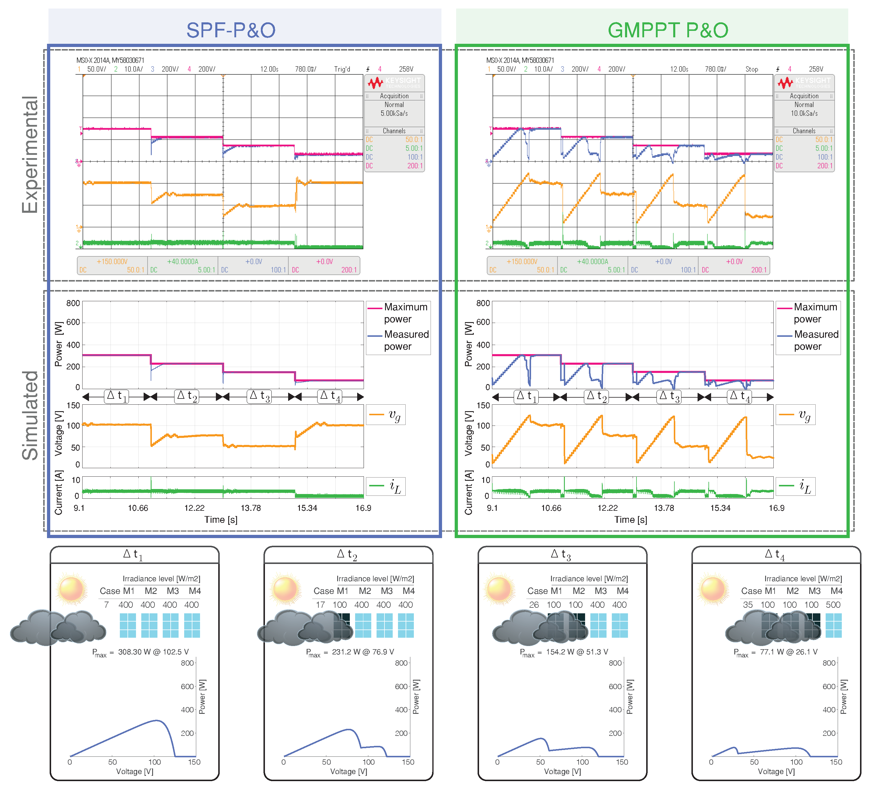
4.3.4. Scenario 4: Multiple Peaks in the P-V Characteristic

Scenario 4 has the sequence of case 3 with only one peak (GMPP), case 52 with two peaks (One GMPP and one LMPP), and case 85 with three peaks (One GMPP and two LMPP) in the P-V characteristic. The results for each MPPT algorithms are shown in Figure 11.

For case 3, the irradiance is uniform with a unique MPP at $104.28$ V, which is tracked faster by the proposed algorithm. When the irradiance changes in case 52, there are two peaks, the proposed algorithm misidentifies the optimum voltage but archived the maximum power.

Finally, when the irradiation is changed in case 85, there are three peaks, where the algorithm has quickly identified and tracked the second peak ($55.3$ V, $81.3$ W) as the GMPP. The SPF-P&O presents an overall GMPPT tracking efficiency of 90.86%, while the GMPPT P&O method presents a tracking efficiency of $79.85$%.

The results for the cases’ sequence are evaluated through standard errors (21)–(23), and the scores of mean power tracked and tracking factor as shown in Figure 12.

From this figure it can inferred that the proposed GMPPT method has high MPP tracking capability regarding to GMPPT P&O method under multiple peaks in the P-V characteristic due to different PSCs.

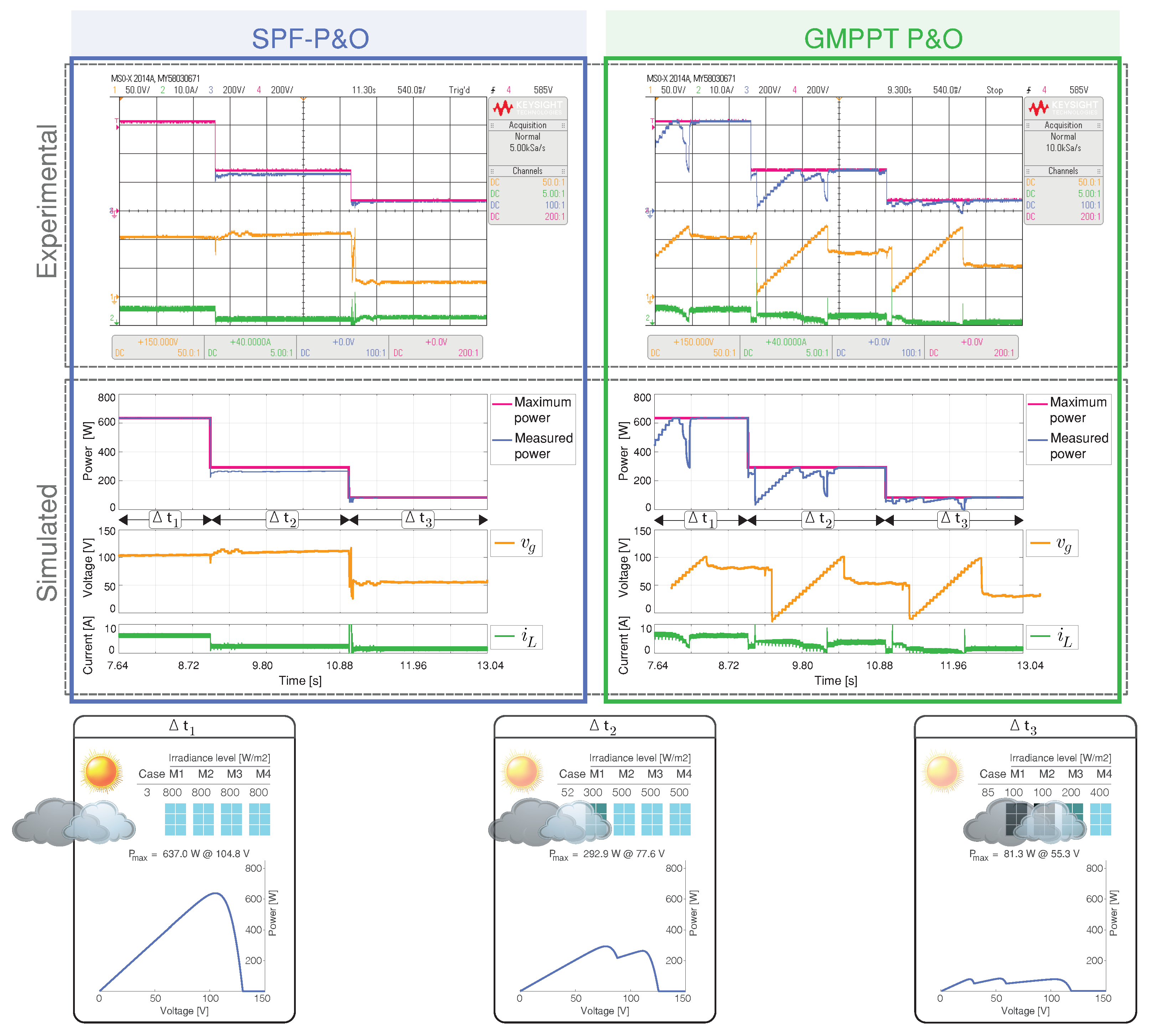
4.3.5. Scenario 5: Dark Cloud Passing

A dark cloud passes in this scenario, obscuring each one of the PV modules. The sequence of the cases included in this scenario correspond to the cases 7, 17, 26, and 35 as presented in Figure 13.

Cases 17, 26 and 35 correspond to (PSCs), which has two peaks, and the proposed GMPPT correctly identifies the optimal voltage for the maximum power point for the transition between cases 7, 17, and 26. Nevertheless, the reference voltage value for case 35 is incorrectly identified by the SPF-P&O algorithm.

This error is because the power between the GMPP ($77.1$ W at $26.1$ V) and the LMPP located in the second peak ($72.26$ W at 100 V) are similar. The proposed MPPT tracked the GMPP much faster than the GMPPT P&O algorithm. Figure 14 shows the standard error and comparison indicators for the results presented in Figure 13.

The SPF-P&O algorithm exhibits smaller error values in comparison to the GMMP P&O method. The SPF-P&O algorithm presents a tracking factor of 93.53% while the GMPPT P&O method a tracking factor of 72.29%.

4.3.6. Scenario 6: Light Cloud Passing

In this scenario a light cloud passes, partially obscuring one by one the PV modules.

The results of scenario 6 has the sequence of cases: 8, 63, 95, and 127, and the results are presented in in Figure 15.

Figure 16 illustrates that the proposed method provides the lowest value error for the results seen in Figure 15.

When the irradiance level is reduced by the transition of the cloud, the SPF-P&O algorithm identifies the new GMPPT power for the different cases without oscillations while the GMPPT P&O method has a big oscillation around the GMPPT, and this is reflected in the current and voltage waveforms.

The SPF-P&O algorithm presents a tracking factor of $97.1$% while for the GMPPT P&O method a value of $76.27$%.

5. Conclusions

A fast-tracking hybrid MPPT technique based on Surface-Based Polynomial Fitting and P&O has been presented for solar PV under PSCs. The SPF-P&O MPPT uses a polynomial model from the characterization of the PV module data, which is evaluated during irradiance variations. Meanwhile, the conventional P&O tracks the MPPT under uniform irradiance. The power circuit model was implemented using an RT BOX 1 tool. A low-cost commercial DSC was used to implement the proposed MPPT algorithm and the double-loop strategies in a C programming software.

As experimentally demonstrated in this work, the introduced SPF-P&O GMPPT approach can tie together the estimation capability of the conventional P&O with a curve-fitting-based approach (namely surface-based polynomial fitting). Thus, it can be said that the hybrid approach represents a synergistic and complementary strategy to leverage the effectiveness of a P&O-type method with global data fitting using a polynomial approach. Different profile tests proved that the proposed hybrid method is robust and performs a faster and more effective MPP tracking with no steady-state oscillations for partial shading conditions.

In the future, a more extensive comparison between different MPPT techniques under PSCs using a low-cost commercial microcontroller will be conducted to accomplish deeper insights about the efficiency of PV systems, furthering the growth of photovoltaics as an affordable and sustainable energy source.

References

1. Murdock, H.E.; Gibb, D.; Andre, T.; Sawin, J.L.; Brown, A.; Ranalder, L.; Collier, U.; Dent, C.; Epp, B.; Hareesh Kumar, C.; et al. Renewables 2021-Global Status Report. 2021. Available online: https://www.ren21.net/wp-content/uploads/2019/05/GSR2021_Full_Report.pdf (accessed on 29 September 2021).
2. Lappalainen, K.; Valkealahti, S. Experimental study of the maximum power point characteristics of partially shaded photovoltaic strings. Appl. Energy 2021, 301, 117436. [Google Scholar] [CrossRef]
3. Hamza Zafar, M.; Mujeeb Khan, N.; Feroz Mirza, A.; Mansoor, M.; Akhtar, N.; Usman Qadir, M.; Ali Khan, N.; Raza Moosavi, S.K. A novel meta-heuristic optimization algorithm based MPPT control technique for PV systems under complex partial shading condition. Sustain. Energy Technol. Assess. 2021, 47, 101367. [Google Scholar] [CrossRef]
4. Chen, X.; Du, Y.; Lim, E.; Wen, H.; Yan, K.; Kirtley, J. Power ramp-rates of utility-scale PV systems under passing clouds: Module-level emulation with cloud shadow modeling. Appl. Energy 2020, 268, 114980. [Google Scholar] [CrossRef]
5. Belhaouas, N.; Cheikh, M.S.A.; Agathoklis, P.; Oularbi, M.R.; Amrouche, B.; Sedraoui, K.; Djilali, N. PV array power output maximization under partial shading using new shifted PV array arrangements. Appl. Energy 2017, 187, 326–337. [Google Scholar] [CrossRef]
6. Bradai, R.; Boukenoui, R.; Kheldoun, A.; Salhi, H.; Ghanes, M.; Barbot, J.P.; Mellit, A. Experimental assessment of new fast MPPT algorithm for PV systems under non-uniform irradiance conditions. Appl. Energy 2017, 199, 416–429. [Google Scholar] [CrossRef]
7. Chao, K.H.; Lin, Y.S.; Lai, U.D. Improved particle swarm optimization for maximum power point tracking in photovoltaic module arrays. Appl. Energy 2015, 158, 609–618. [Google Scholar] [CrossRef]
8. Mohammadinodoushan, M.; Abbassi, R.; Jerbi, H.; Waly Ahmed, F.; Abdalqadir kh ahmed, H.; Rezvani, A. A new MPPT design using variable step size perturb and observe method for PV system under partially shaded conditions by modified shuffled frog leaping algorithm- SMC controller. Sustain. Energy Technol. Assess. 2021, 45, 101056. [Google Scholar] [CrossRef]
9. Laxman, B.; Annamraju, A.; Srikanth, N.V. A grey wolf optimized fuzzy logic based MPPT for shaded solar photovoltaic systems in microgrids. Int. J. Hydrogen Energy 2021, 46, 10653–10665. [Google Scholar] [CrossRef]
10. Fares, D.; Fathi, M.; Shams, I.; Mekhilef, S. A novel global MPPT technique based on squirrel search algorithm for PV module under partial shading conditions. Energy Convers. Manag. 2021, 230, 113773. [Google Scholar] [CrossRef]
11. Houssein, E.H.; Mahdy, M.A.; Fathy, A.; Rezk, H. A modified Marine Predator Algorithm based on opposition based learning for tracking the global MPP of shaded PV system. Expert Syst. Appl. 2021, 183, 115253. [Google Scholar] [CrossRef]
12. González-Castaño, C.; Lorente-Leyva, L.L.; Muñoz, J.; Restrepo, C.; Peluffo-Ordóñez, D.H. An MPPT Strategy Based on a Surface-Based Polynomial Fitting for Solar Photovoltaic Systems Using Real-Time Hardware. Electronics 2021, 10, 206. [Google Scholar] [CrossRef]
13. Ghasemi, M.A.; Foroushani, H.M.; Parniani, M. Partial shading detection and smooth maximum power point tracking of PV arrays under PSC. IEEE Trans. Power Electron. 2015, 31, 6281–6292. [Google Scholar] [CrossRef] [Green Version]
14. Ali, A.; Almutairi, K.; Padmanaban, S.; Tirth, V.; Algarni, S.; Irshad, K.; Islam, S.; Zahir, M.H.; Shafiullah, M.; Malik, M.Z. Investigation of MPPT Techniques Under Uniform and Non-Uniform Solar Irradiation Condition—A Retrospection. IEEE Access 2020, 8, 127368–127392. [Google Scholar] [CrossRef]
15. Bollipo, R.B.; Mikkili, S.; Bonthagorla, P.K. Hybrid, optimal, intelligent and classical PV MPPT techniques: A review. CSEE J. Power Energy Syst. 2021, 7, 9–33. [Google Scholar] [CrossRef]
16. Guest, P.G.; Guest, P.G. Numerical Methods of Curve Fitting; Cambridge University Press: New York, NY, USA, 2012. [Google Scholar]
17. Erickson, R.W.; Maksimovic, D. Fundamentals of Power Electronics, 2nd ed.; Kluwer Academic Publishers: Boston, MA, USA, 2001. [Google Scholar]
18. Hart, D.W. Power Electronics; Tata McGraw-Hill Education: New York, NY, USA, 2010. [Google Scholar]
19. Corradini, L.; Maksimovic, D.; Mattavelli, P.; Zane, R. Digital Control of High-Frequency Switched-Mode Power Converters; Wiley-IEEE Press: Piscataway, NJ, USA, 2015. [Google Scholar]
20. El Aroudi, A.; Martínez-Treviño, B.A.; Vidal-Idiarte, E.; Cid-Pastor, A. Fixed switching frequency digital sliding-mode control of DC-DC power supplies loaded by constant power loads with inrush current limitation capability. Energies 2019, 12, 1055. [Google Scholar] [CrossRef] [Green Version]
21. Vidal-Idiarte, E.; Marcos-Pastor, A.; Garcia, G.; Cid-Pastor, A.; Martinez-Salamero, L. Discrete-time sliding-mode-based digital pulse width modulation control of a boost converter. IET Power Electron. 2015, 8, 708–714. [Google Scholar] [CrossRef]
22. Vidal-Idiarte, E.; Marcos-Pastor, A.; Giral, R.; Calvente, J.; Martinez-Salamero, L. Direct digital design of a sliding mode-based control of a PWM synchronous buck converter. IET Power Electron. 2017, 10, 1714–1720. [Google Scholar] [CrossRef]
23. Farhat, M.; Barambones, O.; Sbita, L. A new maximum power point method based on a sliding mode approach for solar energy harvesting. Appl. Energy 2017, 185, 1185–1198. [Google Scholar] [CrossRef]
24. Kamran, M.; Mudassar, M.; Fazal, M.R.; Asghar, M.U.; Bilal, M.; Asghar, R. Implementation of improved Perturb & Observe MPPT technique with confined search space for standalone photovoltaic system. J. King Saud Univ.-Eng. Sci. 2018, 32, 432–441. [Google Scholar]
25. Kollimalla, S.K.; Mishra, M.K. A novel adaptive P&O MPPT algorithm considering sudden changes in the irradiance. IEEE Trans. Energy Convers. 2014, 29, 602–610. [Google Scholar]
26. Ahmed, J.; Salam, Z. A modified P&O maximum power point tracking method with reduced steady-state oscillation and improved tracking efficiency. IEEE Trans. Sustain. Energy 2016, 7, 1506–1515. [Google Scholar]
27. Chapra, S.C. Applied Numerical Methods with MATLAB for Engineers and Scientists; McGraw-Hill: New York, NY, USA, 2012. [Google Scholar]
28. Tomczyk, K.; Makowski, T.; Kowalczyk, M.; Ostrowska, K.; Beńko, P. Procedure for the Accurate Modelling of Ring Induction Motors. Energies 2021, 14, 5469. [Google Scholar] [CrossRef]
29. Stroock, D.W. Probability Theory: An Analytic View, 2nd ed.; Cambridge University Press: New York, NY, USA, 2010. [Google Scholar]
30. Zafar, M.H.; Al-shahrani, T.; Khan, N.M.; Feroz Mirza, A.; Mansoor, M.; Qadir, M.U.; Khan, M.I.; Naqvi, R.A. Group teaching optimization algorithm based MPPT control of PV systems under partial shading and complex partial shading. Electronics 2020, 9, 1962. [Google Scholar] [CrossRef]
Figure 1. P-V characteristics of four PV module KC200GT under uniform and nonuniform irradiance conditions and connected in series.
Mathematics 09 02732 g001
Figure 2. Plotting of the MPP surface in terms of P p v and v g .
Mathematics 09 02732 g002
Figure 3. Hardware in-the-loop experimental setup: (a) oscilloscope, (b) PLECS RT box, (c) RT box launchPad interface, (d) Texas Instruments LAUNCHXL-F28069M, (e) Laptop.
Mathematics 09 02732 g003
Figure 4. Experimental (a,b), responses of the sliding digital current input control when the reference i r e f : (a) changes from 4 A to 8 A, and (b) from 8 A to 4 A. The converter operates with V g = 100 V and V o = 160 V of input and output voltage, respectively. CH1: V g (60 V/div), CH2: V o (60 V/div), CH3: i L (2A/div) and a time base of 500 μ s. (c) responses of the double-loop using sliding digital current control when the reference v r e f changes with steps of 5 V between 100 V to 110 V while the output voltage ( V o = 160 V) ensures a boost operation. CH1: v g (20 V/div), CH2: V o 20 V/div), CH3: i L (20 A/div) and a time base of 156 ms.
Mathematics 09 02732 g004
Figure 5. Simulated and experimental dynamic behavior of the MPPT algorithms for Scenario 1 and an output voltage V o = 160 V. The proposed MPPT algorithm (left) is compared with GMPPT P&O (right). CH1: v g (50 V/div), CH2: i L (10 A/div), CH3: Maximum power (200 W/div), CH4: Measured power (200 W/div) and a time base of 220 ms.
Mathematics 09 02732 g005
Figure 6. Comparative analysis of the MPPT methods for Scenario 1 shown in Figure 5.
Mathematics 09 02732 g006
Figure 7. Simulated and experimental dynamic behavior of the MPPT algorithms for Scenario 2 with an output voltage V o = 160 V. The proposed MPPT algorithm (right) is compared with the GMPPT P&O algorithm (right). CH1: v g (50 V/div), CH2: i L (10 A/div), CH3: Maximum power (200 W/div), CH4: Measured power (200 W/div) and a time base of 960 ms.
Mathematics 09 02732 g007
Figure 8. Comparative analysis of the MPPT methods under different uniform irradiance conditions for Scenario 2 shown in Figure 7.
Mathematics 09 02732 g008
Figure 9. Simulated and experimental dynamic behavior of the MPPT algorithms for Scenario 3 with an output voltage V o = 160 V. The proposed MPPT algorithm (right) is compared with the GMPPT P&O algorithm (right). CH1: v g (50 V/div), CH2: i L (10 A/div), CH3: Maximum power (200 W/div), CH4: Measured power (200 W/div) and a time base of 450 ms.
Mathematics 09 02732 g009
Figure 10. Comparative analysis of the MPPT methods for Scenario 3 shown in Figure 9.
Mathematics 09 02732 g010
Figure 11. Simulated and experimental dynamic behavior of the MPPT algorithms for Scenario 4 with an output voltage V o = 160 V. The proposed MPPT algorithm (right) is compared with the GMPPT P&O algorithm (right). CH1: v g (50 V/div), CH2: i L (10 A/div), CH3: Maximum power (200 W/div), CH4: Measured power (200 W/div) and a time base of 540 ms.
Mathematics 09 02732 g011
Figure 12. Comparative analysis of the MPPT methods for Scenario 4 shown in Figure 11.
Mathematics 09 02732 g012
Figure 13. Simulated and experimental dynamic behavior of the MPPT algorithms for Scenario 5 with an output voltage V o = 160 V. The proposed MPPT algorithm (right) is compared with the GMPPT P&O algorithm (right). CH1: v g (50 V/div), CH2: i L (10 A/div), CH3: Maximum power (200 W/div), CH4: Measured power (200 W/div) and a time base of 780 ms.
Mathematics 09 02732 g013
Figure 14. Comparative analysis of the MPPT methods under different nonuniform irradiance conditions for Scenario 5 shown in Figure 13.
Mathematics 09 02732 g014
Figure 15. Simulated and experimental dynamic behavior of the MPPT algorithms for Scenario 6 with an output voltage V o = 160 V. The proposed MPPT algorithm (right) is compared with the GMPPT P&O algorithm (right). CH1: v g (50 V/div), CH2: i L (10 A/div), CH3: Maximum power (200 W/div), CH4: Measured power (200 W/div) and a time base of 780 ms.
Mathematics 09 02732 g015
Figure 16. Comparative analysis of the MPPT methods for Scenario 6 shown in Figure 15.
Mathematics 09 02732 g016