Abstract
Weighted belief propagation (WBP) for the decoding of linear block codes is considered. In WBP, the Tanner graph of the code is unrolled with respect to the iterations of the belief propagation decoder. Then, weights are assigned to the edges of the resulting recurrent network and optimized offline using a training dataset. The main contribution of this paper is an adaptive WBP where the weights of the decoder are determined for each received word. Two variants of this decoder are investigated. In the parallel WBP decoders, the weights take values in a discrete set. A number of WBP decoders are run in parallel to search for the best sequence- of weights in real time. In the two-stage decoder, a small neural network is used to dynamically determine the weights of the WBP decoder for each received word. The proposed adaptive decoders demonstrate significant improvements over the static counterparts in two applications. In the first application, Bose–Chaudhuri–Hocquenghem, polar and quasi-cyclic low-density parity-check (QC-LDPC) codes are used over an additive white Gaussian noise channel. The results indicate that the adaptive WBP achieves bit error rates (BERs) up to an order of magnitude less than the BERs of the static WBP at about the same decoding complexity, depending on the code, its rate, and the signal-to-noise ratio. The second application is a concatenated code designed for a long-haul nonlinear optical fiber channel where the inner code is a QC-LDPC code and the outer code is a spatially coupled LDPC code. In this case, the inner code is decoded using an adaptive WBP, while the outer code is decoded using the sliding window decoder and static belief propagation. The results show that the adaptive WBP provides a coding gain of 0.8 dB compared to the neural normalized min-sum decoder, with about the same computational complexity and decoding latency.
1. Introduction
Neural networks (NNs) have been widely studied to improve communication systems. The ability of NNs to learn from data and model complex relationships makes them indispensable tools for tasks such as equalization, monitoring, modulation classification, and beamforming [1]. While NNs have also been considered for decoding error-correcting codes for quite some time [2,3,4,5,6,7,8,9,10], interest in this area has surged significantly in recent years due to advances in NNs and their widespread commercialization [11,12,13,14,15,16,17,18,19,20,21,22,23,24,25,26,27,28,29,30,31,32,33,34,35,36,37,38,39,40,41,42,43,44,45,46].
Two categories of neural decoders may be considered. In model-agnostic decoders, the NN has a general architecture independent of the conventional decoders in coding theory [12,34,42]. Many of the common architectures have been studied for decoding, including multi-layer perceptrons [5,12,47], convolutional NNs (CNNs) [48], recurrent neural networks (RNNs) [13], autoencoders [19,35,40], convolutional decoders [6], graph NNs [33,43], and transformers [34,41]. These models have been used to decode linear block codes [4,12], Reed–Solomon codes [49], convolutional codes [4,48,50], Bose–Chaudhuri–Hocquenghem (BCH) codes [11,16,18,31], Reed–Muller codes [5,25], turbo codes [13], low-density parity-check (LDPC) codes [37,51], and polar codes [52].
Training neural decoders is challenging because the number of codewords to classify depends exponentially on the number of information bits. Furthermore, the sample complexity of the NN is high for the small bit error rates (BERs) and long block lengths required in some applications. As a consequence, model-agnostic decoders often require a large number of parameters and may overfit, which makes them impractical unless the block length is short.
In model-based neural decoders, the architecture of the NN is based on the structure of a conventional decoder [11,14,25,28,31,53]. An example is weighted belief propagation (WBP), where the messages exchanged across the edges of the Tanner graph of the code are weighted and optimized [11,31,54]. This gives rise to a decoder in the form of a recurrent network obtained by unfolding the update equations of the belief propagation (BP) over the iterations. Since the WBP is a biased model, it has fewer parameters than the model-agnostic NNs at the same accuracy.
Prior work has demonstrated that the WBP outperforms BP for block lengths up to around 1000, particularly with structured codes, low-to-moderate code rates, and high signal-to-noise ratios (SNRs) [17,28,31,37,38,39,54,55,56,56]. It is believed that the improvement is achieved by altering the log-likelihood ratios (LLRs) that are passed along short cycles. For example, for BCH and LDPC codes with block lengths under 200, WBP provides frame error rate (FER) improvements of up to 0.4 dB in the waterfall region and up to 1.5 dB in the error-floor region [23,57,58]. Protograph-based (PB) QC-LDPC codes have been similarly decoded using the learned weighted min-sum (WMS) decoder [28].
The WBP does not generalize well at low bit error rates (BERs) due to the requirement of long block lengths and the resulting high sample and training complexity [44]. For example, in optical fiber communication, the block length can be up to tens of thousands to achieve a BER of . In this case, the sample complexity of WBP is high, and the model does not generalize well when trained with a practically manageable number of examples.
The training complexity and storage requirements of the WBP can be reduced through parameter sharing. Lian et al. introduced a WBP decoder wherein the parameters are shared across or within the layers of the NN [18,39]. A number of parameter-sharing schemes in WBP are studied in [28,39]. Despite intensive research in recent years, WBP remains impractical in most real-world applications.
In this work, we improve the generalization of WBP to enhance its practical applicability. The WBP is a static NN, trained offline based on a dataset. The main contribution of this paper is the proposal of adaptive learned message-passing algorithms, where the weights assigned to messages are determined for each received word. In this case, the decoder is dynamic, changing its parameters for each transmission in real time.
Two variants of this decoder are proposed. In the parallel decoder architecture, the weights take values in a discrete set. A number of WMS decoders are run in parallel to find the best sequence of weights based on the Hamming weight of the syndrome of the received word. In the two-stage decoder, a secondary NN is trained to compute the weights to be used in the primary NN decoder. The secondary NN is a CNN that takes the LLRs of the received word and is optimized offline.
The performance and computational complexity of the static and adaptive decoders are compared in two applications. In the first application, a number of regular and irregular quasi-cyclic low-density parity-check (QC-LDPC) codes, along with a BCH and a polar code, are evaluated over an additive white Gaussian noise (AWGN) channel in both low- and high-rate regimes. The results indicate that the adaptive WMS decoders achieve decoding BERs up to an order of magnitude less than the BERs of the static WMS decoders, at about the same decoding complexity, depending on the code, its rate, and the SNR. The coding gain is 0.32 dB at a bit error rate of in one example.
The second application is coding over a nonlinear optical fiber link with wavelength division multiplexing (WDM). The data rates in today’s optical fiber communication system approach terabits/s per wavelength. Here, the complexity, power consumption, and latency of the decoder are important considerations. We apply concatenated coding by combining a low-complexity short-block-length soft-decision inner code with a long-block-length hard-decision outer code. This approach allows the component codes to have much shorter block lengths and higher BERs than the combined code. As a result, it becomes feasible to train the WBP for decoding the inner code, addressing the curse of dimensionality and sample complexity issues. For PB QC-LDPC inner codes and a spatially coupled (SC) QC-LDPC outer code, the results indicate that the adaptive WBP outperforms the static WBP by 0.8 dB at about the same complexity and decoding latency in a 16-QAM 8 × 80 km 32 GBaud WDM system with five channels.
The remainder of this paper is organized as follows. Section 2 introduces the notation, followed by the channel models in Section 3. In Section 4, we introduce the WBP, and in Section 5, two adaptive learned message-passing algorithms. In Section 6, we compare the performance and complexity of the static and adaptive decoders, and in Section 7, we conclude the paper. Appendix A and Appendix B provide supplementary information, and Appendix C presents the parameters of the codes.
2. Notation
Natural, real, complex and non-negative numbers are denoted by , , , and , respectively. The set of integers from m to n is shown as . The special case is shortened to . and denote, respectively, the floor and ceiling of . The Galois field GF(q) with , , is . The set of matrices with m rows, n columns, and elements in is .
A sequence of length n is denoted as . Deterministic vectors are denoted by boldface font, e.g., . The entry of is . Deterministic matrices are shown by upper-case letters with mathrm font, e.g., .
The probability density function (PDF) of a random variable X is denoted by , shortened to if there is no ambiguity. The conditional PDF of Y given X is . The expected value of a random variable X is denoted by . The real Gaussian PDF with mean and standard deviation is denoted by . The Q function is , where is the complementary error function. The binary entropy function is , .
3. Channel Models
3.1. AWGN Channel
Encoder: We consider an binary linear code with the parity-check matrix (PCM) , where n is the code length, k is the code dimension, and , . The rate of the code is . A PB QC-LDPC code is characterized by a lifting factor , a base matrix , and an exponent matrix where, , . Given , the PCM is obtained according to the procedure in Appendix A.
We evaluate a BCH code, seven regular and irregular QC-LDPC codes, and a polar code in the low- and high-rate regimes. These codes are summarized in Table 1 and described in Section 6.1. The parameters of the QC-LDPC codes are given in Appendix C.

Table 1.
Codes in this paper.
The encoder maps a sequence of information bits , , , to a codeword as , where is the generator matrix of the code.
Channel model: The codeword is modulated with a binary phase shift keying with symbols , and transmitted over an AWGN channel. The vector of received symbols is , where
where . If is the SNR, the channel can be normalized so that , and .
The LLR function of conditioned on is
for each . Equation (2) holds under the assumption that are independent and uniformly distributed, and (3) is obtained from Gaussian from (1).
Decoder: We compare the performance and complexity of the static and adaptive belief propagation. The static decoders are tanh-based BP, the auto-regressive BP and WBP with different levels of parameter sharing, including BP with simple scaling and parameter-adapter networks (SS-PAN) [18]. Additionally, to assess the achievable performance with a large number of parameters in the decoder, we include a comparison with two model-agnostic neural decoders based on transformers [41] and graph NNs [33,43].
3.2. Optical Fiber Channel
In this application, we consider a multi-user fiber-optic transmission system using WDM with users, each of bandwidth Hz, as shown in Figure 1.
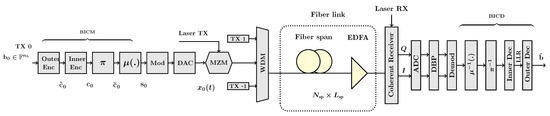
Figure 1.
Block diagram of an optical fiber transmission system.
Transmitter (TX): A binary source generates a pseudo-random bit sequence of information bits , , for the WDM channel , , , . Bit-interleaved coded modulation (BICM) with concatenated coding is applied in WDM channels independently. The BICM comprises an outer encoder for the code with rate , an inner encoder for with rate , a permuter , and a mapper , where is assumed to be an integer. The concatenated code has parameters and and . Each consecutive subsequence of of length is mapped to by the outer encoder and subsequently to by the inner encoder. Next, is mapped to by a random uniform permuter . The mapper maps consecutive sub-sequences of of length m to a symbol in a constellation of size . Thus, the BICM maps to a sequence of symbols , where , , , , .
The symbols are modulated with a root raised cosine (RRC) pulse shape at symbol rate , where t is the time. The resulting electrical signal of each channel is converted to an optical signal and subsequently multiplexed by a WDM multiplexer. The baseband representation of the transmitted signal is
where and are i.i.d. random variables. The average power of the transmitted signal is ; thus, , .
Encoder: SC LDPC codes are attractive options for optical communications [59]. These codes approach the capacity of the canonical communication channels [60,61] and have a flexible performance–complexity trade-off. They are decoded with the BP and the sliding window decoder (SWD). Another class of codes in optical communication is the SC product-like codes, braided block codes [62], SC turbo product codes [63], staircase codes [64,65,66] and their generalizations [67,68]. These codes are decoded with iterative, algebraic hard decision algorithms and prioritize low-complexity, hardware-friendly decoding over coding gain.
In this paper, the encoding in BICM combines an inner (binary or non-binary) QC-LDPC code with an outer SC QC-LDPC code whose component code is a multi-edge QC-LDPC code, as outlined in Table 1. The construction and parameters of the codes are given in Appendix B.1 and Appendix C, respectively.
The choice of the inner code is due to the decoder complexity. Other options have been considered in the literature, for instance, algebraic codes, e.g., the BCH (Section 3.3 [69]) or Reed-Solomon codes (Section 3.4 [69]), or polar codes [70]. However, the QC-LDPC codes are simpler to decode, especially at high rates. The outer code can be an LDPC code [71,72], a staircase code [71,73], or a SC-LDPC code [72].
Fiber-optic link: The channel is an optical fiber link with spans of length of the standard single-mode fiber, with parameters in Table 2.
Table 2.
The parameters of the fiber-optic link.
Let be the complex envelope of the signal as a function of time t and distance z along the fiber. The propagation of the signal in one polarization over one span of optical fiber is modeled by the nonlinear Schrödinger equation [74]
where is the loss constant, is the chromatic dispersion coefficient, is the Kerr nonlinearity parameter, and . The transmitter is located at and the receiver at . The continuous-time model (5) can be discretized to a discrete-time discrete-space model using the split-step Fourier method (Section III.B [75]). The optical fiber channel described by the partial differential Equation (5) differs significantly from the AWGN channel due to the presence of nonlinearity.
An erbium doped fiber amplifier (EDFA) is placed at the end of each span, which compensates for the fiber loss, and introduces amplified spontaneous emission noise. The input –output relation of the EDFA is given by , where is the amplifier’s gain, and is zero-mean circularly symmetric complex Gaussian noise process with the power spectral density
where NF is the noise figure, h is a Planck constant, and is the carrier frequency at 1550 nm.
Receiver: The advent of the coherent detection paved the way for the compensation of transmission effects in optical fiber using digital signal processing (DSP). As a result, the linear effects in the channel, such as the chromatic dispersion and polarization-induced impairments, and some of the nonlinear effects, can be compensated with DSP.
At the receiver, a demultiplexer filters the signal of each WDM channel. The optical signal for each channel is converted to an electrical signal by a coherent receiver. Next, DSP followed by bit-interleaved coded demodulation (BICD) is applied. The continuous-time electrical signal is converted to the discrete-time signals by analogue-to-digital converters, down-sampled, and passed to a digital signal processing unit for the mitigation of the channel impairments. For equalization, digital back-propagation (DBP) based on the symmetric split-step Fourier method is applied to compensate for most of the linear and nonlinear fiber impairments [76].
After DSP, the symbols are still subject to signal-dependent noise, which is mitigated by the bit-interleaved coded demodulator (BICD). Let denote the equalized signal samples for the transmitted symbols in the WDM channel of interest. Given that the deterministic effects were equalized, we assume that the channel is memoryless so that . For , let . From the symbol-to-symbol channel , , , we obtain m bit-to-symbol channels
where , and .
Let , . The LLR function of conditioned on is, for each ,
where is obtained from i according to , , and is defined in (6).
Decoder: The decoding of consists of two steps. First, is decoded using an adaptive WBP in Appendix B, which takes the soft information and corrects some errors. Second, is decoded using the min-sum (MS) decoder with SWD in Appendix B, which further lowers the BER, and outputs the decoded information bits . The LLRs in the inner decoder are represented with 32 bits, and in the outer decoder are quantized at 4 bits with per-window configuration.
In optical communication, the forward error correction (FEC) overhead 6–25% is common [77]. Thus, the inner code typically has a high rate of ≥0.9 and a block length of several thousands, achieving a BER of –. The outer code has a length of up to tens of thousands, lowering the BER to an error floor to ∼.
3.3. Performance Metrics
Q-factor: The SNR per bit in the optical fiber channel is , where is the bit energy, and is the total noise power in the link, where . The performance of the uncoded communication system is often measured by the BER. The Q-factor for a given BER is the corresponding SNR in an additive white Gaussian noise channel with binary phase-shift keying modulation:
Coding gain: Let and (respectively, and ) denote the BER and Q-factor at the input (respectively, output) of the decoder. The coding gain (CG) in dB is the reduction in the Q-factor
The corresponding net CG (NCG) is
Finite block-length NCG: If n is finite, the rate in (8) may be replaced with the information rate in the finite block-length regime [78]
where
4. Weighted Belief Propagation
Given a code , one can construct a bipartite Tanner graph , where , , , and are, respectively, the set of check nodes, variable nodes and the edges connecting them. Let , , and and be the degree of c and v in , respectively.
The WBP is an iterative decoder based on the exchange of the weighted LLRs between the variable nodes and the check nodes in [11,79]. Let denote the extrinsic LLR from the check node c to the variable node v at iteration t. Define similarly .
The decoder is initialized at with , where v is the j-th variable node, and is obtained from (3) or (7). For iteration , the LLRs are updated in two steps.
The check node update:
where
The equation in represents the update relation in the BP [69], where the LLR messages are scaled by non-negative weights . Further, is obtained from though an approximation to lower the computational cost. The WBP and WMS decoders use and , respectively.
The variable-node update:
This is the update relation in the BP, to which the sets of non-negative weights and are introduced.
At the end of each iteration t, a hard decision is made
where
Let , and let be the syndrome. The algorithm stops if or .
The computation in (9) and (10) can be expressed with an NN. The Tanner graph is unrolled over the iterations to obtain a recurrent network with layers (see Figure 2), in which the weights and are assigned to the edges of , and the weights to the outputs [16]. The weights are obtained by minimizing a loss function evaluated over a training dataset using the standard optimizers for NNs.
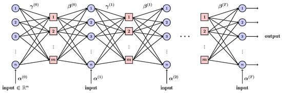
Figure 2.
Tanner graph unrolled to an RNN.
4.1. Parameter Sharing Schemes
The training complexity of WBP can be reduced through parameter sharing at the cost of performance loss. We consider dimensions for the ragged arrays and . In Type T parameter sharing over , parameters are shared with respect to iterations t. In Type scheme, , , . In this case, there is a single ragged array with trainable parameters . For the regular LDPC code, . It has been observed that for typical block lengths, indeed, the weights do not change significantly with iterations [28]. In Type , there are T arrays , while in Type , there are two arrays and . Type and decoders can be referred to as BP-RNN decoders and Type as feedforward BP. In Type V sharing, is independent of v. This corresponds to one weight per check node. Likewise, in Type C sharing, there is one weight per check node update, and .
These schemes can be combined. For instance, in Type parameter sharing, . Thus, a single parameter is introduced in all layers of the NN. This decoder is referred to as the neural normalized BP, e.g., neural normalized min-sum (NNMS) decoder when BP is based on the MS algorithm. The latter is similar to the normalized MS decoder, except that the parameter is empirically determined there. In the Type scheme, . Here, there is one weight per iteration. In this paper, .
4.2. WBP over
The construction and decoding of the PB QC-LDPC binary codes can be extended to codes over a finite field [80,81]. Here, there are LLR messages sent from each node, defined in Equation (1) [81]. The update equations of the BP are similar to (9)–(10), and presented in [81] for the extended min-sum (EMS) and in [82] for the weighted EMS (WEMS) decoder.
The parameter sharing for the four-dimensional ragged array is defined in Section 4.1. In the check-node update of the WEMS algorithm, it is possible to assign a distinct weight to each coefficient for every variable node. For instance, in the Type scheme, and , so there is one weight per variable and one per check node . In the case of Type , there is only one weight per variable, iteration, and coefficient. In this case, if BP is based on the non-binary EMS algorithm, the decoder is called the neural normalized EMS (NNEMS).
Remark 1.
The EMS decoder has a truncation factor in that provides a trade-off between complexity and accuracy. In this paper, it is set to q to investigate the maximum performance.
5. Adaptive Learned Message Passing Algorithms
The weights of the static WBP are obtained by training the network offline using a dataset. A WBP where the weights are determined for each received word is an adaptive WBP. The weights must therefore be found by online optimization. To manage the complexity, we consider a WMS decoder with Type parameter sharing. Thus, the decoder has one weight per T iterations, which must be determined for a received .
Let be a codeword and be the corresponding received word, where for the AWGN channel and for the optical fiber channel. Let be the word decoded by a Type WBP decoder with weight in iteration , where . In the adaptive decoder, we wish to find a function , , that minimizes the probability that makes an error
where is a functional class. The static decoder is a special case where is a constant function. Two variants of this decoder are proposed, illustrated in Figure 3.
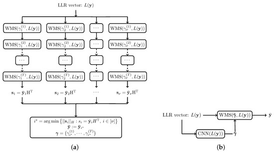
Figure 3.
Adaptive decoders. (a) Parallel decoders; (b) the two-stage decoder. refers to .
5.1. Parallel Decoders
Architecture: In parallel decoders, is found through searching. Here, takes value in a discrete set , , and thus . The parallel decoders consist of independent decoders , , running concurrently. Since in (13) is generally intractable, a sub-optimal is selected as follows. At the end of decoding by , the syndrome is computed. Let
be the index of the decoder whose syndrome has the smallest Hamming weight. Then, , and .
In practice, the search can be performed up to depth iterations. However, the BP decoder often has to run for more iterations. Thus, a WBP decoder with weights can continue the output with iterations.
Remark 2.
The decoder obtained via (14) is generally sub-optimal. Minimizing does not necessarily minimize the number of errors. However, for random codes, the decoder obtained from (14) outperforms the static decoder.
Remark 3.
If and yield the same number of errors, the decoder with the smaller weight vector is selected, which tends to output smaller LLRs.
Obtaining from the distribution of weights.: The values of can be determined by dividing a sub-interval in uniformly. The resulting parallel WMS decoder outperforms WMS; however, the performance can be improved by choosing based on the probability distribution of the weights.
The probability distribution of the channel noise induces a distribution on and consequently on . Let be a random variable representing . Denote the corresponding mean by , standard deviation by , and the cumulative distribution function by . For , set
The numbers partition the real line into intervals such that and . In practice, has a distribution close to Gaussian, in which case values are given by the explicit formulas in Lemma 1.
Lemma 1.
Let have a cumulative distribution function that is continuous and strictly monotonic. For ,
If has a Gaussian distribution with a mean and standard deviation , then
where erfc is the complementary error function.
Proof.
The proof is based on elementary calculus. □
Obtaining the distribution of weights: To apply (15) or (16), is required. To this end, a static WBP (with no parameter sharing) is trained offline given a dataset . The empirical cumulative distribution of the weights in each iteration is computed as an approximation to . However, if the BER is low, it can be difficult to obtain a dataset that contains a sufficient number of examples corresponding to incorrectly decoded words required to obtain good generalization.
To address this issue, we apply active learning [23,83]. This approach is based on the fact that the training examples near the decision boundary of the optimal classifier determine the classifier the most. Hence, input examples are sampled from a probability distribution with a support near the decision boundary.
The following approach to active learning is considered. At epoch e in the training of the WBP, random codewords and the corresponding outputs are computed. The decoder from the epoch is applied to decode to . An acquisition function evaluates whether the example pair should be retained. A candidate example is retained if is in a given range.
The choice of the acquisition function depends on the specific problem being solved, the architecture of the NN, and the availability of the labeled data [83]. In the context of training the NN decoders for channel coding, the authors of [23] use distance parameters and reliability parameters. Inspired by [23], the authors of [84] define the acquisition function using importance sampling. In this paper, the acquisition function is the number of errors , where is the Hamming distance.
The dataset is incrementally generated and pruned as follows. At each epoch e, a subset of examples, filtered by the acquisition function, is selected. The entire dataset at epoch e is and has size . The operator Prune removes the subsets introduced in old epochs if and otherwise leaves its input intact. At each epoch e, the loss function is averaged over a batch set of size obtained by randomly sampling from .
Complexity of the parallel decoders: The computational complexity of the decoder is measured in real multiplications (RMs). For instance, the complexity of the WMS with T iterations, , without parameter sharing, or with Type parameter sharing, is , where is the number of edges of the Tanner graph of the code. For the WMS decoder with Type or Type parameter sharing, . The latter arises from the fact that equal weights factor out of the ∑ and the min terms in BP and are applied once. Thus, the complexity of ν parallel WMS decoders with Type parameter sharing is . If , is added to the above formulas. Finally, the complexity of Type decoder is RM per single iteration. These expressions neglect the cost of the syndrome check.
5.2. Two-Stage Decoder
In a parallel decoder, the weights are restricted in a discrete set. The number of parallel decoders depends exponentially on the size of this set. The two-stage decoder predicts arbitrary non-negative weights, without the exponential complexity of the parallel decoders. Further, since the weights are arbitrary, the two-stage decoder can improve upon the performance of the parallel decoders, when the output LLRs are sensitive to the weights.
Architecture: Recall that we wish to find a function that minimizes the BER in (13). In a two-stage decoder, this function is expressed by an NN parameterized by vector θ. Thus, the two-stage decoder is a combination of an NN and a WBP. First, the NN takes as input either the LLRs at the channel output or and outputs the vector of weights . Then, the WBP decoder takes the channel LLRs and weights and outputs the decoded word .
The parameters θ are found using a dataset of examples , where is the target weight. This dataset can be obtained through a simulation, i.e., transmitting a codeword , receiving , and using, e.g., an offline parallel decoder to determine the target weight . In this manner, is expressed in a functional form instead of being determined by real-time search, which may be more expensive.
In this paper, the NN is a CNN consisting of a cascade of two one-dimensional convolutional layers and , followed by a dense layer . applies filters of size and stride 1, and the rectified linear unit (ReLU) activation, . The output of is flattened and passed to , which produces the vector of weights of length T. This final layer is a linear transformation with ReLU activation to produce non-negative weights.
The model is trained by minimizing the quantile loss function
where is the quantile parameter and max is applied per entry and mean over vector entries. The choice of loss is obtained by cross-validating the validation error over a number of candidate functions. This is an asymmetric absolute-like loss, which, if as in Section 6, encourages entries of to be close to entries of γ from above rather than below.
Complexity of the two-stage decoder: The computational complexity of the two-stage decoder in the inference mode is the sum of the complexity of the CNN and WMS decoder
where the computational complexity of the CNN is
The complexity can be significantly reduced by pruning the weights, for example, by setting to zero the weights below a threshold .
Remark 4.
Neural decoders are sensitive to distribution shifts and often require retraining when the input distribution or channel conditions change. To lower the training complexity, [18] proposed a decoder that learns a mapping from the input SNR to the weights in WBP, enabling the decoder to operate across a range of SNRs. However, the WBP decoder in [18] is static, since the weights remain fixed throughout the transmission once chosen, despite being referred to as dynamic WBP. We do not address the problem of distribution shift in this paper.
6. Performance and Complexity Comparison
In this section, we study the performance and complexity trade-off of the static and adaptive decoders for the AWGN in Section 3.1 and optical fiber channel in Section 3.2.
6.1. AWGN Channel
Low-rate regime: To investigate the error correction performance of the decoders at low rates, we consider a BCH code of rate with the cycle-reduced parity check matrix in [85] and two QC-LDPC codes and , which are, respectively, - and -regular with rates of and . The parity check matrix of each QC-LDPC code is constructed using an exponent matrix obtained from the random progressive edge growth (PEG) algorithm [86], with a girth-search depth of two, which is subsequently refined manually to remove the short cycles in their Tanner graphs. The parameters of the QC-LDPC codes, including the exponent matrices and , are given in Appendix C. In addition, we consider the irregular LDPC codes specified in the 5G New Radio (NR) standard and in the Consultative Committee for Space Data Systems (CCSDS) standard [85]. The code parameters, such as exponent matrices, are also available in the public repository ([87] v0.1).
We compare our adaptive decoders with tanh-based BP, the auto-regressive BP and several static WMS decoder with different levels of parameter sharing, such as BP with SS-PAN [18]. The latter is a Type WBP with , i.e., a BP with two parameters. Additionally, to assess the achievable performance with a large number of parameters in the decoder, we include a comparison with two model-agnostic neural decoders based on the transformer [41] and graph NNs [33,43].
The number of iterations in the WMS decoders of the parallel decoders is chosen so that the total computational complexities of the parallel decoders and the static WMS decoder are about the same. In Figure 4a, this value is for , where is the total number of iterations; in Figure 4b–d, for and , for , and for ; in Figure 4f, for . Furthermore, for all .
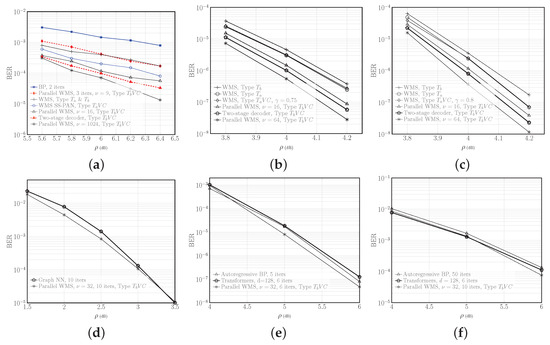
Figure 4.
BER versus SNR ρ, for the AWGN channel in the low-rate regime. (a) BCH code . Here, the curve for WMS, Type & is from ([16] Figure 8) and the curve for WMS SS-PAN is from ([18] Figure 5a). (b) QC-LDPC code , (c) QC-LDPC code , (d) 5G-NR LDPC code . Here, the curve for Graph NN is from ([33] Figure 5). (e) CCSDS LDPC code . In this and the next sub-figure, the Autoregressive BP and Transformers curves are from [30] and [34], respectively. (f) BCH code . Figures (d–f) show that adaptive decoders achieve the performance of the static decoders with less complexity.
To compute the value of weights , the probability distribution of is required. For this purpose, a WMS decoder is trained offline. The training dataset is a collection of examples obtained using the AWGN channel with a range of SNRs dB for or dB for and . The datasets for and are obtained similarly, with different sets of SNRs. The acquisition function in active learning is the Hamming distance. A candidate example for the training dataset is retained if . The parameters of the active learning are , and 40,000. The loss function is the binary cross-entropy. The models are trained using the Adam optimizer with a learning rate of . It is observed that the distribution of is nearly Gaussian. Thus, we obtain from (16). Table 3 presents the mean and variance of this distribution, and , for the three codes considered.
Table 3.
The mean and variance of in WMS for the AWGN channel.
For the two-stage decoder, we use a CNN with , , , and , determined by cross-validation. The CNN is trained with a dataset of size 80,000, batch set size 300, and the quantile loss function with . The number of iterations of the WMS decoder for each code is the same as above.
Figure 4 illustrates the BER vs. SNR for different codes, and different decoders for the same code. In each of Figure 4a–d, one can compare different decoders at about the same complexity (except for the parallel decoder with the largest ν that shows the smallest achievable BER). For instance, it can be seen in Figure 4a that the two-stage decoder achieves half the BER of the WMS with SS-PAN decoder at SNR dB for the short length code , or approximately dB gain in SNR at a BER of . For this code, the parallel WMS decoders with 3 iterations and outperforms the tanh-based BP with nearly the same complexity. Figure 4b,c show that the two-stage decoder offers about an order-of-magnitude improvement in the BER compared to the Type WMS decoder at dB for moderate-length codes and , or over dB gain at a BER of . The performance gains vary with the code, parameters, and SNR.
Figure 4d–f compare decoders with different complexities at about the same performance. The proposed adaptive model-based decoders achieve the same performance of the model-agnostic static decoders, with far fewer parameters.
The computational complexity of the decoders are presented in Table 4. For the CNN, from (17), , which is further reduced by a factor of 4 upon pruning at the threshold , with minimal impact on BER. Thus, the two-stage decoder requires less than half of the RM of the WMS decoder with no or Type parameter sharing. Moreover, the two-stage decoder requires approximately one-fifth of the RM of the parallel decoders with . Compared to the WMS decoder with SS-PAN [18], the two-stage decoder has nearly double the complexity, albeit with much lower BER, as seen in Figure 4a.
Table 4.
Computational complexity of decoders, for the AWGN channel.
High-rate regime: To further investigate the error correction performance of the decoders at high rates, we consider three single-edge QC-LDPC codes, , , and , associated, respectively, with the PCMs , , and . These codes have rates , , and , respectively, and are constructed using the PEG algorithm. The PEG algorithm requires the degree distributions of the Tanner graph, which are optimized using the stochastic extrinsic information transfer (EXIT) chart described in Appendix C. Additionally, we include the polar code with from the 5G-NR standard as a state-of-the-art benchmark. The code parameters, including degree distribution polynomials and the exponent matrices, are given in Appendix C.
The acquisition function with active learning in the parallel decoders is based on Figure 5. The figure shows the scatter plot of the pre-FEC error versus post-FEC error , for 340 examples for at dB. Here, is the hard decision of the LLRs at the channel output defined in (11), and is decoded with the best decoder at epoch e, i.e., the WMS with weights from epoch . The acquisition function retains if (no error) or if falls in the rectangle in Figure 5 (with error). The rectangle is defined such that . It is ensured that 70% of examples satisfy and 30% with in the rectangle . In this example, , and , , . We use , 20,000, and the learning rate .
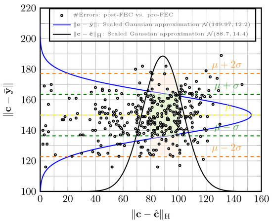
Figure 5.
The scatter plot of for at dB, for the AWGN channel. The scaled Gaussian approximation curve is fitted per axis.
For the adaptive decoder, we consider five parallel decoders with iterations. The decoder for the binary codes , and is WMS with Type sharing. The output of the decoder with the smallest syndrome is continued with an MS decoder with iterations. The polar code, however, is decoded with either a cyclic redundancy check (CRC) and successive cancellation list (SCL) with list size L [88] or the optimized successive cancellation (OSC) [89].
Figure 6 shows the performance of the adaptive and static MS decoders for , and . The polar code with 24 CRC bits is simulated using AFF3CT software toolbox ([90] v3.0.2). It can be seen that at high SNRs, , and decoded with adaptive parallel decoders outperform . Given this, and the higher complexity of decoding the polar code with either SCL or OSC [88], the choice of QC-LDPC codes for the inner code for the optical fiber channel in Section 6.2 is justified.
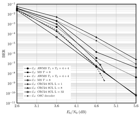
Figure 6.
Performance of the polar code versus QC-LDPC codes and , for the AWGN channel in the high-rate regime. The curve for OSC decoder is from [89].
Figure 7 shows the performance of with rate . The adaptive WMS decoder with iterations outperforms the static MS decoder with iterations at by an order of magnitude in BER.
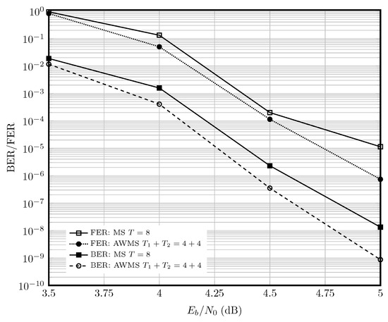
Figure 7.
Performance of the static and adaptive MS decoder for at dB, for the AWGN channel in the high-rate regime.
The gains of WBP depend on parameters such as the block length or SNR [91] (Section IV. d [44]). In general, the gain is decreased when the block length is increased, with other parameters remaining fixed.
6.2. Optical Fiber Channel
We simulate a 16-QAM WDM optical communication system described in Section 3.2, with parameters described in Table 2. The continuous-time model (5) is simulated with the split-step Fourier method with a spatial step size of 100 m and a simulation bandwidth of 200 GHz. DBP with two samples/symbol is applied to compensate for the physical effects and to obtain the per-symbol channel law , , . For the inner code in the concatenated code, we consider two QC-LDPC codes of rate : binary single-edge code and non-binary multi-edge code over , respectively, with PCMs and , given in Appendix C. For the component code used in the outer spatially coupled code, we consider multi-edge QC-LDPC code with the PCM . For and , the resulting SC-QC-LDPC code has the PCM , where is the spreading matrix. The outer SC-QC-LDPC code is encoded with the sequential encoder [92]. This requires that the top-left block of in Equation (A2) is of full rank. Thus, is designed to fulfill this condition. In Equation (A2), we have , , is of full rank, and . The rate of the component code is , and the rate of outer SC code is , so . The and matrices are constructed heuristically and are given in Appendix C.
The inner code is decoded with the parallel decoder, with five decoders with four iterations each. The decoder for the binary code is WMS with Type parameter sharing, while for the non-binary code, is WEMS with Type sharing and . The static EMS algorithm [93] is parameterized as in Section 4, initialized with the LLRs computed from Equation (1) [81]. The outer code is decoded with the SWD, with the static MS decoding of a maximum of 26 iterations per window.
Table 5 and Table 6 contain a summary of the numerical results. is pre-FEC BER, and the reference BER for the coding gain is . dBm, the total gap to NCGf for the adaptive weighted min-sum AWSM (resp., WEMS) decoder is 2.51 (resp., 1.75), while this value is 3.31 (resp., 2.29) and 3.44 (resp., 2.69), respectively, for the NNMS (resp., NNEMS) and MS (resp., EMS) decoders. Thus, the adaptive WBP provides a coding gain of 0.8 dB compared to the static NNMS decoder with about the same computational complexity and decoding latency
Table 5.
Concatenated inner binary QC-LDPC code and outer SC-QC-LDPC code with an for the optical fiber channel. The sections for 0.012 and 0.025 correspond to average powers −10 and −11 dBm, respectively. NCGs are in dB.
Table 6.
Concatenated inner non-binary QC-LDPC code and outer SC-QC-LDPC code with for the optical fiber channel. The sections for 0.012 and 0.025 correspond to average powers −10 and −11 dBm, respectively. NCGs are in dB.
7. Conclusions
Adaptive decoders are proposed for codes on graphs that can be decoded with message-passing algorithms. Two variants, the parallel WBP and the two-stage decoder, are studied. The parallel decoders search for the best sequence of weights in real time using multiple instances of the WBP decoder running concurrently, while the two-stage neural decoder employs an NN to dynamically determine the weights of WBP for each received word. The performance and complexity of the adaptive and several static decoders are compared for a number of codes over an AWGN and optical fiber channel. The simulations show that significant improvements in BER can be obtained using adaptive decoders, depending on the channel, SNR, the code and its parameters. Future work could explore further reducing the computational complexity of the online learning, and applying adaptive decoders to other types of codes and wireless channels.
Author Contributions
Conceptualization, A.T. and M.Y.; Methodology, A.T. and M.Y.; Software, A.T. and M.Y.; Formal analysis, A.T. and M.Y.; Investigation, A.T. and M.Y.; Writing—original draft, A.T. and M.Y.; Project administration, M.Y. All authors have read and agreed to the published version of the manuscript.
Funding
This work has received funding from the European Research Council (ERC) research and innovation program, under the COMNFT project, Grant Agreement no. 805195.
Institutional Review Board Statement
Not applicable.
Data Availability Statement
Data is contained within the article.
Conflicts of Interest
The authors declare no conflicts of interest.
Abbreviations
The following abbreviations are used in this manuscript.
| AWGN | Additive White Gaussian Noise |
| AWEMS | Adaptive Weighted Extended Min-sum |
| AWMS | Adaptive Weighted Min-sum |
| BCH | Bose–Chaudhuri–Hocquenghem |
| BER | Bit Error Rate |
| BICD | Bit-interleaved Coded Demodulation |
| BICM | Bit-interleaved Coded Modulation |
| BP | Belief Propagation |
| CG | Coding Gain |
| CNN | Convolutional Neural Network |
| CRC | Cyclic Redundancy Check |
| DSP | Digital Signal Processing |
| EDFA | Erbium Doped Fiber Amplifier |
| EMS | Extended Min-sum |
| EXIT | Extrinsic Information Transfer |
| FEC | Forward Error Correction |
| FER | Frame Error Rate |
| GF | Galois Field |
| LDPC | Low-density Parity-check |
| LLR | Log-likelihood Ratio |
| MS | Min-sum |
| NCG | Net Coding Gain |
| NF | Noise Figure |
| NN | Neural Network |
| NR | New Radio |
| NNEMS | Neural Normalized Extended Min-sum |
| NNMS | Neural Normalized Min-sum |
| OSC | Optimized Successive Cancellation |
| PB | Protograph-based |
| PCM | Parity-check Matrix |
| Probability Density Function | |
| PEG | Progressive-edge Growth |
| QAM | Quadrature Amplitude Modulation |
| QC | Quasi-cyclic |
| ReLU | Rectified Linear Unit |
| RRC | Root Raised Cosine |
| RM | Real Multiplication |
| RNN | Recurrent Neural Network |
| SC | Spatially coupled |
| SS-PAN | Simple Scaling and Parameter-adapter Networks |
| SCL | Successive Cancellation List |
| SWD | Sliding Window Decoder |
| WBP | Weighted Belief Propagation |
| WDM | Wavelength Division Multiplexing |
| WEMS | Weighted Extended Min-sum |
| WMS | Weighted Min-sum |
Appendix A. Protograph-Based QC-LDPC Codes
In this appendix and the next, we provide the supplementary information necessary to reproduce the results presented in this paper. The presentation in Appendix B may be of independent interest, as it provides an accessible exposition of the construction and decoding of the SC codes.
Appendix A.1. Construction for the Single-Edge Case
A single-edge PB QC-LDPC code is constructed in two steps. First, a base matrix is constructed, where , . Then, is expanded to the PCM of by replacing each zero in with the all-zero matrix , where is the lifting factor, and a one in row i and column j with a sparse circulant matrix .
Let be the exponent matrix of the code, with the entries denoted by . The matrices (and ) can be obtained from as follows. Denote by , the circulant permutation matrix obtained by cyclic-shifting of each row of the identity matrix n positions to the right, with the convention that is the all-zero matrix. Then, . The PCM of this QC-LDPC code is
This code has a length , , and a rate , where is the rank of . If is of a full rank, . The base matrix is also obtained from , as if and if .
Denote the Tanner graph of by , and let and be, respectively, the degree of the check node c and the variable node v in . If is regular (i.e., its rows have the same Hamming weight), then is regular, and the check and variable nodes of have the same degrees and , respectively. In this case, is said to be -regular. More generally, a variable node’s degree distribution polynomial can be defined as , where is the fraction of variable nodes of degree d, and a check node degree distribution , where is the fraction of check nodes of degree d.
The parameter matrices and can be obtained so as to maximize the girth of using search-based methods such as the PEG algorithm [86,94], algebraic methods ([69] Section 10), or a combination of them [95].
Example A1.
Consider , , and the base matrix
For any exponent matrix , is
Appendix A.2. Construction for the Multi-Edge Case
The above construction can be extended to multi-edge PB QC-LDPC codes. Here, , instead of a binary number, is a sequence of length with entries in . Likewise, is a sequence of length with entries , . Then, . This code is represented by a Tanner graph where there are multiple edges of different types between the variable and the check nodes. We say this code has type . A single-edge PB QC-LDPC code is type 1.
Example A2.
Consider , ,
Then
Appendix A.3. Construction for Non-Binary Codes
In the non-binary codes, the entries of codewords, parity-check, and generator matrices are in a finite field , where q is a power of a prime. There are several ways to construct non-binary PB QC-LDPC codes. The base matrix typically remains binary, as defined as in Appendix A.1. We use the unconstrained and random assignment strategy in [80] to extend to a PCM.
There is significant flexibility in selecting the edge weights for constructing non-binary QC-LDPC codes, which can be classified as constrained or unconstrained ([80] Section II). In this work, we focus on an unconstrained and random assignment strategy, where each edge in corresponding to a 1 in the binary matrix B is replaced with a coefficient . Alternatively, these coefficients could be selected based on predefined rules to ensure appropriate edge-weight diversity, which can lead to enhanced performance. This methodology allows non-binary codes to retain the structural benefits of binary QC-LDPC codes while extending their functionality to finite fields, offering improved error-correcting capabilities for larger q values.
Appendix A.4. Encoder and Decoder
The generator matrix of the code is obtained by applying Gaussian elimination in the binary field to (A1). The encoder is then implemented efficiently using shift registers [96].
The QC-LDPC codes are typically decoded using belief propagation (BP), as described in Section 4.
Appendix B. Spatially Coupled LDPC Codes
Appendix B.1. Construction
The SC-QC-LDPC codes in this paper are constructed based on the edge spreading process [97]. Denote the PCM of the constituent PB QC-LDPC code by . Denote the PCM of the corresponding SC-QC-LDPC code by , with the additional parameters of the syndrome memory , coupling length , and the spreading matrix . Then, is given by
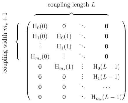 in which are block matrices, , and is obtained from as
where .
in which are block matrices, , and is obtained from as
where .
in which are block matrices, , and is obtained from asIf , and , the code is time-invariant. If and are full-rank, then the rate of SC-QC-LDPC code is , where is the rate of the component QC-LDPC code. For a fixed , as , then . Thus, the rate loss in SC-LDPC codes can be reduced by increasing the coupling length.
Example A3.
Consider any QC-LDPC code, , and the spreading matrix
Then, is obtained by replacing each entry of that is 2 at row i and column j with , and other entries with . Thus, for all
In a similar manner,
If is full-rank, then . If is also full-rank, then and . □
The SC-LDPC code is efficiently encoded sequentially [92] so that at each spatial position ℓ, information bits are encoded out of .
If an entry of corresponding to an is a sequence, the corresponding entry in is also a sequence. Thus, if represents a multi-edge code for some i or ℓ, so does .

Figure A1.
(a) A window in SWD is a block, each block with size . The window slides diagonally by one block. The variable nodes in the block at the block-position are denoted by , and the check nodes by . Here, and . (b) The message update for the current window ℓ is denoted by the solid rectangle. The variable nodes in the previous windows and not in the current window ℓ, denoted in green, send fixed messages to the check nodes in the current window in any iterations t. The blue variable nodes in the current and a previous window send to the check nodes in the current window at iteration , which would be updated according to (9) and (10) for . The red variable nodes in the current window, but not in any previous window, send to the check nodes in the current window at , which would be updated at . The edges from the gray check nodes in windows are discarded for the decoding at position ℓ.
Appendix B.2. Encoder
The SC-LDPC codes are encoded with the sequential encoder [92].
Appendix B.3. Sliding Window Decoder
Consider the SC LDPC code in Appendix B.1. Note that any two variable-nodes in the Tanner graph of the code whose corresponding columns in are at least columns apart do not share any common check-nodes. Thus, they are not involved in the same parity-check equation. The SWD uses this property and runs a local BP decoder on windows of shown in Figure A1.
SWD works through a sequence of spatial iterations ℓ, where a rectangular window slides from the top-left to the bottom-right side of . In general, a window matrix of size consists of consecutive rows and consecutive columns in . At each iteration ℓ, it moves rows down and columns to the right in . Thus, a window is an block, starting from the top left and moving diagonally one block down per iteration. There is a special case where the window reaches the boundary. The way the windows near the boundary are terminated impacts performance [98,99]. Our setup for window termination at boundary is early termination, which is discussed in section III-B1 [99].
Denote the variable nodes in window ℓ by
The check-nodes directly connected to are . Define (the variable nodes in the previous windows not in the current window, shown in green in Figure A1) (the variable nodes in the current window and any previous window, shown in blue in Figure A1), and (the variables nodes in the current window not in any previous window, shown in red in Figure A1). Let and be LLRs in window ℓ and iteration in BP. At , the BP is initialized as
The update equation for the variable node is
The update relation for is given by (9), with no weights, applied for and . After iterations, the variables in the window ℓ, called target symbols, are decoded. The SWD is illustrated in Figure A1.
Appendix C. Parameters of Codes
For low-rate codes, first, the degree distributions of the Tanner graph are determined using the extrinsic information transfer (EXIT) chart [100]. The EXIT chart produces accurate results if [100]. For high-rate codes, we apply the stochastic EXIT chart, which in the short block length regime yields better coding gains compared to the deterministic variant [101]. For instance, while the EXIT chart suggests that the degree distributions of are optimal near dB, the stochastic EXIT chart in Figure A2 suggests dB. Indeed, at dB, the check-node extrinsic information intersects with variable-node extrinsic information for the deterministic EXIT chart. The exponent matrices are obtained using the PEG algorithm, which takes the optimized degree distribution polynomials.
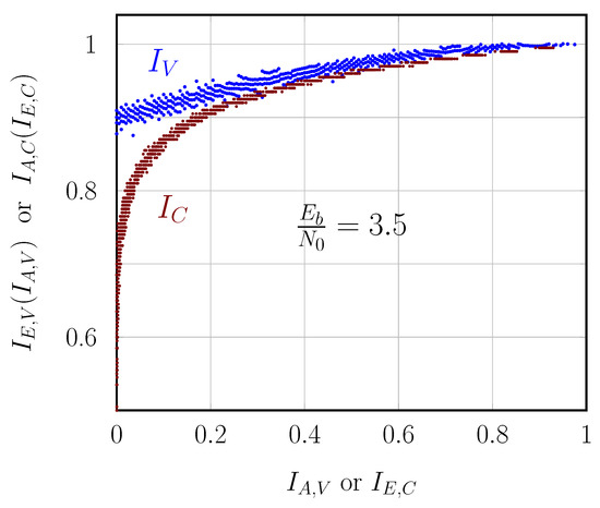
Figure A2.
Stochastic EXIT chart for the high-rate code at dB, for the AWGN channel.
The matrices below are vectorized row-wise. They can be unvectorized considering their dimensions.
: , , , , , below
: , , , , , below
: , , , , , below
: , , , ,
, below
: , , , ,
, below
: , , , ,
, below
: , , , , , below
: , , ,
, below
, below
References
- Pham, Q.V.; Nguyen, N.T.; Huynh-The, T.; Bao Le, L.; Lee, K.; Hwang, W.J. Intelligent radio signal processing: A survey. IEEE Access 2021, 9, 83818–83850. [Google Scholar] [CrossRef]
- Bruck, J.; Blaum, M. Neural networks, error-correcting codes, and polynomials over the binary n-cube. IEEE Trans. Inf. Theory 1989, 35, 976–987. [Google Scholar] [CrossRef]
- Zeng, G.; Hush, D.; Ahmed, N. An application of neural net in decoding error-correcting codes. In Proceedings of the 1989 IEEE International Symposium on Circuits and Systems (ISCAS), Portland, OR, USA, 8–11 May 1989; Volume 2, pp. 782–785. [Google Scholar] [CrossRef]
- Caid, W.; Means, R. Neural network error correcting decoders for block and convolutional codes. In Proceedings of the GLOBECOM ’90: IEEE Global Telecommunications Conference and Exhibition, San Diego, CA, USA, 2–5 December 1990; Volume 2, pp. 1028–1031. [Google Scholar]
- Tseng, Y.H.; Wu, J.L. Decoding Reed-Muller codes by multi-layer perceptrons. Int. J. Electron. Theor. Exp. 1993, 75, 589–594. [Google Scholar] [CrossRef]
- Marcone, G.; Zincolini, E.; Orlandi, G. An efficient neural decoder for convolutional codes. Eur. Trans. Telecommun. Relat. Technol. 1995, 6, 439–445. [Google Scholar]
- Wang, X.A.; Wicker, S. An artificial neural net Viterbi decoder. IEEE Trans. Commun. 1996, 44, 165–171. [Google Scholar] [CrossRef]
- Tallini, L.G.; Cull, P. Neural nets for decoding error-correcting codes. In Proceedings of the IEEE Technical Applications Conference and Workshops. Northcon/95. Conference Record, Portland, OR, USA, 10–12 October 1995; pp. 89–94. [Google Scholar] [CrossRef]
- Ibnkahla, M. Applications of neural networks to digital communications—A survey. Signal Process. 2000, 80, 1185–1215. [Google Scholar] [CrossRef]
- Haroon, A. Decoding of Error Correcting Codes Using Neural Networks. Ph.D. Thesis, Blekinge Institute of Technology, Blekinge, Sweden, 2012. Available online: https://www.diva-portal.org/smash/get/diva2:832503/FULLTEXT01.pdf (accessed on 11 June 2025).
- Nachmani, E.; Be’ery, Y.; Burshtein, D. Learning to decode linear codes using deep learning. In Proceedings of the 54th Annual Allerton Conference on Communication, Control, and Computing (Allerton), Monticello, IL, USA, 27–30 September 2016; pp. 341–346. [Google Scholar] [CrossRef]
- Gruber, T.; Cammerer, S.; Hoydis, J.; Brink, S.T. On deep learning-based channel decoding. In Proceedings of the 2017 51st Annual Conference on Information Sciences and Systems (CISS), Baltimore, MD, USA, 22–24 March 2017; pp. 1–6. [Google Scholar] [CrossRef]
- Kim, H.; Jiang, Y.; Rana, R.B.; Kannan, S.; Oh, S.; Viswanath, P. Communication algorithms via deep learning. In Proceedings of the International Conference on Learning Representations, Vancouver, BC, Canada, 30 April–3 May 2018; Available online: https://openreview.net/forum?id=ryazCMbR- (accessed on 11 June 2025).
- Vasić, B.; Xiao, X.; Lin, S. Learning to decode LDPC codes with finite-alphabet message passing. In Proceedings of the 2018 Information Theory and Applications Workshop (ITA), San Diego, CA, USA, 11–16 February 2018; pp. 1–9. [Google Scholar]
- Bennatan, A.; Choukroun, Y.; Kisilev, P. Deep learning for decoding of linear codes—A syndrome-based approach. In Proceedings of the 2018 IEEE International Symposium on Information Theory (ISIT), Vail, CO, USA, 17–22 June 2018; pp. 1595–1599. [Google Scholar] [CrossRef]
- Nachmani, E.; Marciano, E.; Lugosch, L.; Gross, W.J.; Burshtein, D.; Be’ery, Y. Deep learning methods for improved decoding of linear codes. IEEE J. Sel. Top. Signal Process. 2018, 12, 119–131. [Google Scholar] [CrossRef]
- Lugosch, L.P. Learning Algorithms for Error Correction. Master’s Thesis, McGill University, Montreal, QC, Canada, 2018. Available online: https://escholarship.mcgill.ca/concern/theses/c247dv63d (accessed on 11 June 2025).
- Lian, M.; Carpi, F.; Häger, C.; Pfister, H.D. Learned belief-propagation decoding with simple scaling and SNR adaptation. In Proceedings of the 2019 IEEE International Symposium on Information Theory (ISIT), Paris, France, 7–12 July 2019; pp. 161–165. [Google Scholar] [CrossRef]
- Jiang, Y.; Kannan, S.; Kim, H.; Oh, S.; Asnani, H.; Viswanath, P. DEEPTURBO: Deep Turbo decoder. In Proceedings of the 2019 IEEE 20th International Workshop on Signal Processing Advances in Wireless Communications (SPAWC), Cannes, France, 2–5 July 2019; pp. 1–5. [Google Scholar] [CrossRef]
- Carpi, F.; Häger, C.; Martalò, M.; Raheli, R.; Pfister, H.D. Reinforcement learning for channel coding: Learned bit-flipping decoding. In Proceedings of the 2019 57th Annual Allerton Conference on Communication, Control, and Computing (Allerton), Monticello, IL, USA, 24–27 September 2019; pp. 922–929. [Google Scholar] [CrossRef]
- Wang, Q.; Wang, S.; Fang, H.; Chen, L.; Chen, L.; Guo, Y. A model-driven deep learning method for normalized Min-Sum LDPC decoding. In Proceedings of the 2020 IEEE International Conference on Communications Workshops (ICC Workshops), Dublin, Ireland, 7–11 June 2020; pp. 1–6. [Google Scholar] [CrossRef]
- Huang, L.; Zhang, H.; Li, R.; Ge, Y.; Wang, J. AI coding: Learning to construct error correction codes. IEEE Trans. Commun. 2020, 68, 26–39. [Google Scholar] [CrossRef]
- Be’Ery, I.; Raviv, N.; Raviv, T.; Be’Ery, Y. Active deep decoding of linear codes. IEEE Trans. Commun. 2020, 68, 728–736. [Google Scholar] [CrossRef]
- Xu, W.; Tan, X.; Be’ery, Y.; Ueng, Y.L.; Huang, Y.; You, X.; Zhang, C. Deep learning-aided belief propagation decoder for Polar codes. IEEE J. Emerg. Sel. Top. Circuits Syst. 2020, 10, 189–203. [Google Scholar] [CrossRef]
- Buchberger, A.; Häger, C.; Pfister, H.D.; Schmalen, L.; i Amat, A.G. Pruning and quantizing neural belief propagation decoders. IEEE J. Sel. Areas Commun. 2021, 39, 1957–1966. [Google Scholar] [CrossRef]
- Dai, J.; Tan, K.; Si, Z.; Niu, K.; Chen, M.; Poor, H.V.; Cui, S. Learning to decode protograph LDPC codes. IEEE J. Sel. Areas Commun. 2021, 39, 1983–1999. [Google Scholar] [CrossRef]
- Tonnellier, T.; Hashemipour, M.; Doan, N.; Gross, W.J.; Balatsoukas-Stimming, A. Towards practical near-maximum-likelihood decoding of error-correcting codes: An overview. In Proceedings of the ICASSP 2021—2021 IEEE International Conference on Acoustics, Speech and Signal Processing (ICASSP), Toronto, ON, Canada, 6–11 June 2021; pp. 8283–8287. [Google Scholar] [CrossRef]
- Wang, L.; Chen, S.; Nguyen, J.; Dariush, D.; Wesel, R. Neural-network-optimized degree-specific weights for LDPC MinSum decoding. In Proceedings of the 2021 11th International Symposium on Topics in Coding (ISTC), Montreal, QC, Canada, 30 August–3 September 2021; pp. 1–5. [Google Scholar] [CrossRef]
- Habib, S.; Beemer, A.; Kliewer, J. Belief propagation decoding of short graph-based channel codes via reinforcement learning. IEEE J. Sel. Areas Inf. Theory 2021, 2, 627–640. [Google Scholar] [CrossRef]
- Nachmani, E.; Wolf, L. Autoregressive belief propagation for decoding block codes. arXiv 2021, arXiv:2103.11780. [Google Scholar]
- Nachmani, E.; Be’ery, Y. Neural decoding with optimization of node activations. IEEE Commun. Lett. 2022, 26, 2527–2531. [Google Scholar] [CrossRef]
- Cammerer, S.; Ait Aoudia, F.; Dörner, S.; Stark, M.; Hoydis, J.; Ten Brink, S. Trainable communication systems: Concepts and prototype. IEEE Trans. Commun. 2020, 68, 5489–5503. [Google Scholar] [CrossRef]
- Cammerer, S.; Hoydis, J.; Aoudia, F.A.; Keller, A. Graph neural networks for channel decoding. In Proceedings of the 2022 IEEE Globecom Workshops (GC Wkshps), Rio de Janeiro, Brazil, 4–8 December 2022; pp. 486–491. [Google Scholar] [CrossRef]
- Choukroun, Y.; Wolf, L. Error correction code transformer. Conf. Neural Inf. Proc. Syst. 2022, 35, 38695–38705. Available online: https://proceedings.neurips.cc/paper_files/paper/2022/file/fcd3909db30887ce1da519c4468db668-Paper-Conference.pdf (accessed on 11 June 2025).
- Jamali, M.V.; Saber, H.; Hatami, H.; Bae, J.H. ProductAE: Toward training larger channel codes based on neural product codes. In Proceedings of the ICC 2022—IEEE International Conference on Communications, Seoul, Republic of Korea, 16–20 May 2022; pp. 3898–3903. [Google Scholar] [CrossRef]
- Dörner, S.; Clausius, J.; Cammerer, S.; ten Brink, S. Learning joint detection, equalization and decoding for short-packet communications. IEEE Trans. Commun. 2022, 71, 837–850. [Google Scholar] [CrossRef]
- Li, G.; Yu, X.; Luo, Y.; Wei, G. A bottom-up design methodology of neural Min-Sum decoders for LDPC codes. IET Commun. 2023, 17, 377–386. [Google Scholar] [CrossRef]
- Wang, Q.; Liu, Q.; Wang, S.; Chen, L.; Fang, H.; Chen, L.; Guo, Y.; Wu, Z. Normalized Min-Sum neural network for LDPC decoding. IEEE Trans. Cogn. Commun. Netw. 2023, 9, 70–81. [Google Scholar] [CrossRef]
- Wang, L.; Terrill, C.; Divsalar, D.; Wesel, R. LDPC decoding with degree-specific neural message weights and RCQ decoding. IEEE Trans. Commun. 2023, 72, 1912–1924. [Google Scholar] [CrossRef]
- Clausius, J.; Geiselhart, M.; Ten Brink, S. Component training of Turbo Autoencoders. In Proceedings of the 2023 12th International Symposium on Topics in Coding (ISTC), Brest, France, 4–8 September 2023; pp. 1–5. [Google Scholar] [CrossRef]
- Choukroun, Y.; Wolf, L. A foundation model for error correction codes. In Proceedings of the International Conference on Learning Representations, Vienna, Austria, 7–11 May 2024; Available online: https://openreview.net/forum?id=7KDuQPrAF3 (accessed on 15 March 2012).
- Choukroun, Y.; Wolf, L. Learning linear block error correction codes. arXiv 2024, arXiv:2405.04050. [Google Scholar]
- Clausius, J.; Geiselhart, M.; Tandler, D.; Brink, S.T. Graph neural network-based joint equalization and decoding. In Proceedings of the 2024 IEEE International Symposium on Information Theory (ISIT), Athens, Greece, 7–12 July 2024; pp. 1203–1208. [Google Scholar] [CrossRef]
- Adiga, S.; Xiao, X.; Tandon, R.; Vasić, B.; Bose, T. Generalization bounds for neural belief propagation decoders. IEEE Trans. Inf. Theory 2024, 70, 4280–4296. [Google Scholar] [CrossRef]
- Kim, T.; Sung Park, J. Neural self-corrected Min-Sum decoder for NR LDPC codes. IEEE Commun. Lett. 2024, 28, 1504–1508. [Google Scholar] [CrossRef]
- Ninkovic, V.; Kundacina, O.; Vukobratovic, D.; Häger, C.; i Amat, A.G. Decoding Quantum LDPC Codes Using Graph Neural Networks. In Proceedings of the GLOBECOM 2024—2024 IEEE Global Communications Conference, Cape Town, South Africa, 8–12 December 2024; pp. 3479–3484. [Google Scholar]
- Cammerer, S.; Gruber, T.; Hoydis, J.; Ten Brink, S. Scaling deep learning-based decoding of Polar codes via partitioning. In Proceedings of the GLOBECOM 2017—2017 IEEE Global Communications Conference, Singapore, 4–8 December 2017; pp. 1–6. [Google Scholar] [CrossRef]
- Sagar, V.; Jacyna, G.M.; Szu, H. Block-parallel decoding of convolutional codes using neural network decoders. Neurocomputing 1994, 6, 455–471. [Google Scholar] [CrossRef]
- Hussain, M.; Bedi, J.S. Reed-Solomon encoder/decoder application using a neural network. Proc. SPIE 1991, 1469, 463–471. [Google Scholar] [CrossRef]
- Alston, M.D.; Chau, P.M. A neural network architecture for the decoding of long constraint length convolutional codes. In Proceedings of the 1990 IJCNN International Joint Conference on Neural Networks, San Diego, CA, USA, 17–21 June 1990; pp. 121–126. [Google Scholar] [CrossRef]
- Wu, X.; Jiang, M.; Zhao, C. Decoding optimization for 5G LDPC codes by machine learning. IEEE Access 2018, 6, 50179–50186. [Google Scholar] [CrossRef]
- Miloslavskaya, V.; Li, Y.; Vucetic, B. Neural network-based adaptive Polar coding. IEEE Trans. Commun. 2024, 72, 1881–1894. [Google Scholar] [CrossRef]
- Doan, N.; Hashemi, S.A.; Mambou, E.N.; Tonnellier, T.; Gross, W.J. Neural belief propagation decoding of CRC-polar concatenated codes. In Proceedings of the ICC 2019—2019 IEEE International Conference on Communications (ICC), Shanghai, China, 20–24 May 2019; pp. 1–6. [Google Scholar]
- Yang, C.; Zhou, Y.; Si, Z.; Dai, J. Learning to decode protograph LDPC codes over fadings with imperfect CSIs. In Proceedings of the 2023 IEEE Wireless Communications and Networking Conference (WCNC), Glasgow, UK, 26–29 March 2023; pp. 1–6. [Google Scholar] [CrossRef]
- Wang, M.; Li, Y.; Liu, J.; Guo, T.; Wu, H.; Lau, F.C. Neural layered min-sum decoders for cyclic codes. Phys. Commun. 2023, 61, 102194. [Google Scholar] [CrossRef]
- Raviv, T.; Goldman, A.; Vayner, O.; Be’ery, Y.; Shlezinger, N. CRC-aided learned ensembles of belief-propagation polar decoders. In Proceedings of the ICASSP 2024—2024 IEEE International Conference on Acoustics, Speech and Signal Processing (ICASSP), Seoul, Republic of Korea, 14–19 April 2024; pp. 8856–8860. [Google Scholar]
- Raviv, T.; Raviv, N.; Be’ery, Y. Data-driven ensembles for deep and hard-decision hybrid decoding. In Proceedings of the 2020 IEEE International Symposium on Information Theory (ISIT), Los Angeles, CA, USA, 21–26 June 2020; pp. 321–326. [Google Scholar] [CrossRef]
- Kwak, H.Y.; Yun, D.Y.; Kim, Y.; Kim, S.H.; No, J.S. Boosting learning for LDPC codes to improve the error-floor performance. In Proceedings of the 37th Conference on Neural Information Processing Systems (NeurIPS 2023), New Orleans, LA, USA, 10–16 December 2023; Volume 36, pp. 22115–22131. Available online: https://proceedings.neurips.cc/paper_files/paper/2023/file/463a91da3c832bd28912cd0d1b8d9974-Paper-Conference.pdf (accessed on 11 June 2025).
- Schmalen, L.; Suikat, D.; Rösener, D.; Aref, V.; Leven, A.; ten Brink, S. Spatially coupled codes and optical fiber communications: An ideal match? In Proceedings of the 2015 IEEE 16th International Workshop on Signal Processing Advances in Wireless Communications (SPAWC), Stockholm, Sweden, 28 June–1 July 2015; pp. 460–464. [Google Scholar] [CrossRef]
- Kudekar, S.; Richardson, T.; Urbanke, R.L. Spatially coupled ensembles universally achieve capacity under belief propagation. IEEE Trans. Inf. Theory 2013, 59, 7761–7813. [Google Scholar] [CrossRef]
- Liga, G.; Alvarado, A.; Agrell, E.; Bayvel, P. Information rates of next-generation long-haul optical fiber systems using coded modulation. IEEE J. Lightw. Technol. 2017, 35, 113–123. [Google Scholar] [CrossRef]
- Feltstrom, A.J.; Truhachev, D.; Lentmaier, M.; Zigangirov, K.S. Braided block codes. IEEE Trans. Inf. Theory 2009, 55, 2640–2658. [Google Scholar] [CrossRef]
- Montorsi, G.; Benedetto, S. Design of spatially coupled Turbo product codes for optical communications. In Proceedings of the 2021 11th International Symposium on Topics in Coding (ISTC), Montreal, QC, Canada, 30 August–3 September 2021; pp. 1–5. [Google Scholar] [CrossRef]
- Smith, B.P.; Farhood, A.; Hunt, A.; Kschischang, F.R.; Lodge, J. Staircase codes: FEC for 100 Gb/s OTN. IEEE J. Lightw. Technol. 2012, 30, 110–117. [Google Scholar] [CrossRef]
- Zhang, L.M.; Kschischang, F.R. Staircase codes with 6% to 33% overhead. IEEE J. Lightw. Technol. 2014, 32, 1999–2002. [Google Scholar] [CrossRef]
- Zhang, L. Analysis and Design of Staircase Codes for High Bit-Rate Fibre-Optic Communication. Ph.D. Thesis, University of Toronto, Toronto, ON, Canada, 2017. Available online: https://tspace.library.utoronto.ca/bitstream/1807/79549/3/Zhang_Lei_201706_PhD_thesis.pdf (accessed on 11 June 2025).
- Shehadeh, M.; Kschischang, F.R.; Sukmadji, A.Y. Generalized staircase codes with arbitrary bit degree. In Proceedings of the 2024 Optical Fiber Communications Conference and Exhibition (OFC), San Diego, CA, USA, 24–28 March 2024; pp. 1–3. Available online: https://ieeexplore.ieee.org/abstract/document/10526860 (accessed on 11 June 2025).
- Sukmadji, A.Y.; Martínez-Peñas, U.; Kschischang, F.R. Zipper codes. IEEE J. Lightw. Technol. 2022, 40, 6397–6407. [Google Scholar] [CrossRef]
- Ryan, W.; Lin, S. Channel Codes: Classical and Modern; Cambridge University Press: Cambridge, UK, 2009; Available online: https://www.cambridge.org/fr/universitypress/subjects/engineering/communications-and-signal-processing/channel-codes-classical-and-modern?format=HB&isbn=9780521848688 (accessed on 11 June 2025).
- Ahmad, T. Polar Codes for Optical Communications. Ph.D. Thesis, Bilkent University, Ankara, Turkey, 2016. Available online: https://api.semanticscholar.org/CorpusID:116423770 (accessed on 11 June 2025).
- Barakatain, M.; Kschischang, F.R. Low-complexity concatenated LDPC-staircase codes. IEEE J. Lightw. Technol. 2018, 36, 2443–2449. [Google Scholar] [CrossRef]
- i Amat, A.G.; Liva, G.; Steiner, F. Coding for optical communications—Can we approach the Shannon limit with low complexity? In Proceedings of the 45th European Conference on Optical Communication (ECOC 2019), Dublin, Ireland, 22–26 September 2019; pp. 1–4. [Google Scholar] [CrossRef]
- Zhang, L.M.; Kschischang, F.R. Low-complexity soft-decision concatenated LDGM-staircase FEC for high-bit-rate fiber-optic communication. IEEE J. Lightw. Technol. 2017, 35, 3991–3999. [Google Scholar] [CrossRef]
- Agrawal, G.P. Nonlinear Fiber Optics, 6th ed.; Academic Press: San Francisco, CA, USA, 2019. [Google Scholar]
- Kramer, G.; Yousefi, M.I.; Kschischang, F. Upper bound on the capacity of a cascade of nonlinear and noisy channels. arXiv 2015, arXiv:1503.07652, 1–4. [Google Scholar]
- Secondini, M.; Rommel, S.; Meloni, G.; Fresi, F.; Forestieri, E.; Poti, L. Single-step digital backpropagation for nonlinearity mitigation. Photonic Netw. Commun. 2016, 31, 493–502. [Google Scholar] [CrossRef]
- Union, I.T. G.709: Interface for the Optical Transport Network (OTN). 2020. Available online: https://www.itu.int/rec/T-REC-G.709/ (accessed on 11 June 2025).
- Polyanskiy, Y.; Poor, H.V.; Verdu, S. Channel coding rate in the finite blocklength regime. IEEE Trans. Inf. Theory 2010, 56, 2307–2359. [Google Scholar] [CrossRef]
- Mezard, M.; Montanari, A. Information, Physics, and Computation; Oxford University Press: Oxford, UK, 2009. [Google Scholar]
- Dolecek, L.; Divsalar, D.; Sun, Y.; Amiri, B. Non-binary protograph-based LDPC codes: Enumerators, analysis, and designs. IEEE Trans. Inf. Theory 2014, 60, 3913–3941. [Google Scholar] [CrossRef]
- Boutillon, E.; Conde-Canencia, L.; Al Ghouwayel, A. Design of a GF(64)-LDPC decoder based on the EMS algorithm. IEEE Trans. Circ. Syst. I 2013, 60, 2644–2656. [Google Scholar] [CrossRef]
- Liang, Y.; Lam, C.T.; Wu, Q.; Ng, B.K.; Im, S.K. A model-driven deep learning-based non-binary LDPC decoding algorithm. TechRxiv 2024. [Google Scholar] [CrossRef]
- Fu, Y.; Zhu, X.; Li, B. A survey on instance selection for active learning. Knowl. Inf. Syst. 2013, 35, 249–283. [Google Scholar] [CrossRef]
- Noghrei, H.; Sadeghi, M.R.; Mow, W.H. Efficient active deep decoding of linear codes using importance sampling. IEEE Commun. Lett. 2024. [Google Scholar] [CrossRef]
- Helmling, M.; Scholl, S.; Gensheimer, F.; Dietz, T.; Kraft, K.; Ruzika, S.; Wehn, N. Database of Channel Codes and ML Simulation Results. 2024. Available online: https://rptu.de/channel-codes/ml-simulation-results (accessed on 11 June 2025).
- Hu, X.Y.; Eleftheriou, E.; Arnold, D.M. Progressive edge-growth Tanner graphs. In Proceedings of the GLOBECOM’01. IEEE Global Telecommunications Conference (Cat. No.01CH37270), San Antonio, TX, USA, 25–29 November 2001; Volume 2, pp. 995–1001. [Google Scholar] [CrossRef]
- Tasdighi, A.; Yousefi, M. The Repository for the Papers on the Adaptive Weighted Belief Propagation. 2025. Available online: https://github.com/comsys2/adaptive-wbp (accessed on 11 June 2025).
- Tal, I.; Vardy, A. List decoding of Polar codes. IEEE Trans. Inf. Theory 2015, 61, 2213–2226. [Google Scholar] [CrossRef]
- Süral, A.; Sezer, E.G.; Kolağasıoğlu, E.; Derudder, V.; Bertrand, K. Tb/s Polar successive cancellation decoder 16 nm ASIC implementation. arXiv 2020, arXiv:2009.09388. [Google Scholar]
- Cassagne, A.; Hartmann, O.; Léonardon, M.; He, K.; Leroux, C.; Tajan, R.; Aumage, O.; Barthou, D.; Tonnellier, T.; Pignoly, V.; et al. AFF3CT: A fast forward error correction toolbox. SoftwareX 2019, 10, 100345. [Google Scholar] [CrossRef]
- Tang, Y.; Zhou, L.; Zhang, S.; Chen, C. Normalized Neural Network for Belief Propagation LDPC Decoding. In Proceedings of the 2021 IEEE International Conference on Networking, Sensing and Control (ICNSC), Xiamen, China, 3–5 December 2021. [Google Scholar]
- Tazoe, K.; Kasai, K.; Sakaniwa, K. Efficient termination of spatially-coupled codes. In Proceedings of the 2012 IEEE Information Theory Workshop, Lausanne, Switzerland, 3–7 September 2012; pp. 30–34. [Google Scholar] [CrossRef]
- Takasu, T. PocketSDR. 2024. Available online: https://github.com/tomojitakasu/PocketSDR/tree/master/python (accessed on 11 June 2025).
- Li, Z.; Kumar, B.V. A class of good quasi-cyclic low-density parity check codes based on progressive edge growth graph. In Proceedings of the Conference Record of the Thirty-Eighth Asilomar Conference on Signals, Systems and Computers, Pacific Grove, CA, USA, 7–10 November 2004; Volume 2, pp. 1990–1994. [Google Scholar] [CrossRef]
- Tasdighi, A.; Boutillon, E. Integer ring sieve for constructing compact QC-LDPC codes with girths 8, 10, and 12. IEEE Trans. Inf. Theory 2022, 68, 35–46. [Google Scholar] [CrossRef]
- Li, Z.; Chen, L.; Zeng, L.; Lin, S.; Fong, W. Efficient encoding of quasi-cyclic low-density parity-check codes. IEEE Trans. Commun. 2006, 54, 71–81. [Google Scholar] [CrossRef]
- Mitchell, D.G.; Rosnes, E. Edge spreading design of high rate array-based SC-LDPC codes. In Proceedings of the 2017 IEEE International Symposium on Information Theory (ISIT), Aachen, Germany, 25–30 June 2017; pp. 2940–2944. [Google Scholar] [CrossRef]
- Lentmaier, M.; Prenda, M.M.; Fettweis, G.P. Efficient message passing scheduling for terminated LDPC convolutional codes. In Proceedings of the 2011 IEEE International Symposium on Information Theory Proceedings, St. Petersburg, Russia, 31 July–5 August 2011; pp. 1826–1830. [Google Scholar] [CrossRef]
- Ali, I.; Kim, J.H.; Kim, S.H.; Kwak, H.; No, J.S. Improving windowed decoding of SC LDPC codes by effective decoding termination, message reuse, and amplification. IEEE Access 2018, 6, 9336–9346. [Google Scholar] [CrossRef]
- Land, I. Code Design with EXIT Charts. 2013. Available online: https://api.semanticscholar.org/CorpusID:61966354 (accessed on 11 June 2025).
- Koike-Akino, T.; Millar, D.S.; Kojima, K.; Parsons, K. Stochastic EXIT design for low-latency short-block LDPC codes. In Proceedings of the 2020 Optical Fiber Communications Conference and Exhibition (OFC), San Diego, CA, USA, 8–12 March 2020; pp. 1–3. Available online: https://ieeexplore.ieee.org/document/9083080 (accessed on 11 June 2025).
Disclaimer/Publisher’s Note: The statements, opinions and data contained in all publications are solely those of the individual author(s) and contributor(s) and not of MDPI and/or the editor(s). MDPI and/or the editor(s) disclaim responsibility for any injury to people or property resulting from any ideas, methods, instructions or products referred to in the content. |
© 2025 by the authors. Licensee MDPI, Basel, Switzerland. This article is an open access article distributed under the terms and conditions of the Creative Commons Attribution (CC BY) license (https://creativecommons.org/licenses/by/4.0/).