
Adaptive Learned Belief Propagation for Decoding Error-Correcting Codes


Abstract
1. Introduction
2. Notation
3. Channel Models
3.1. AWGN Channel
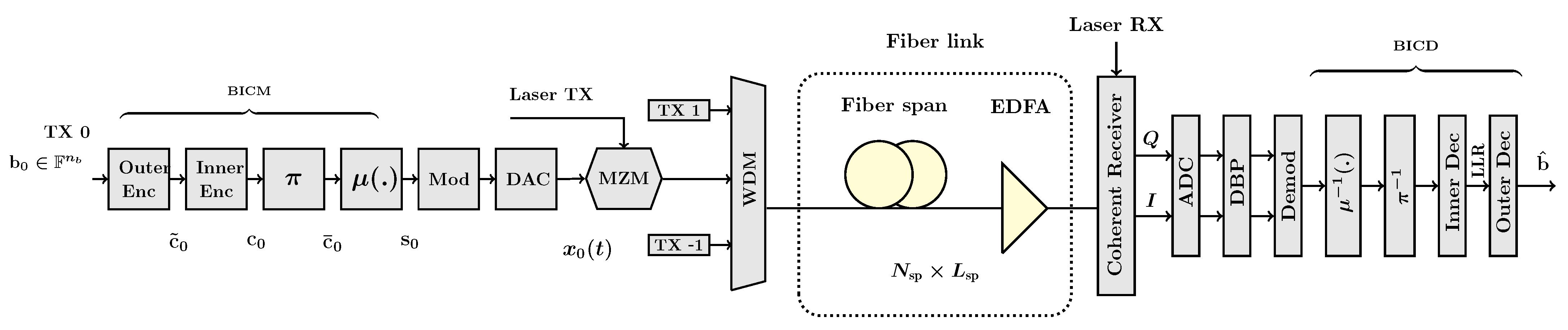
3.2. Optical Fiber Channel
3.3. Performance Metrics
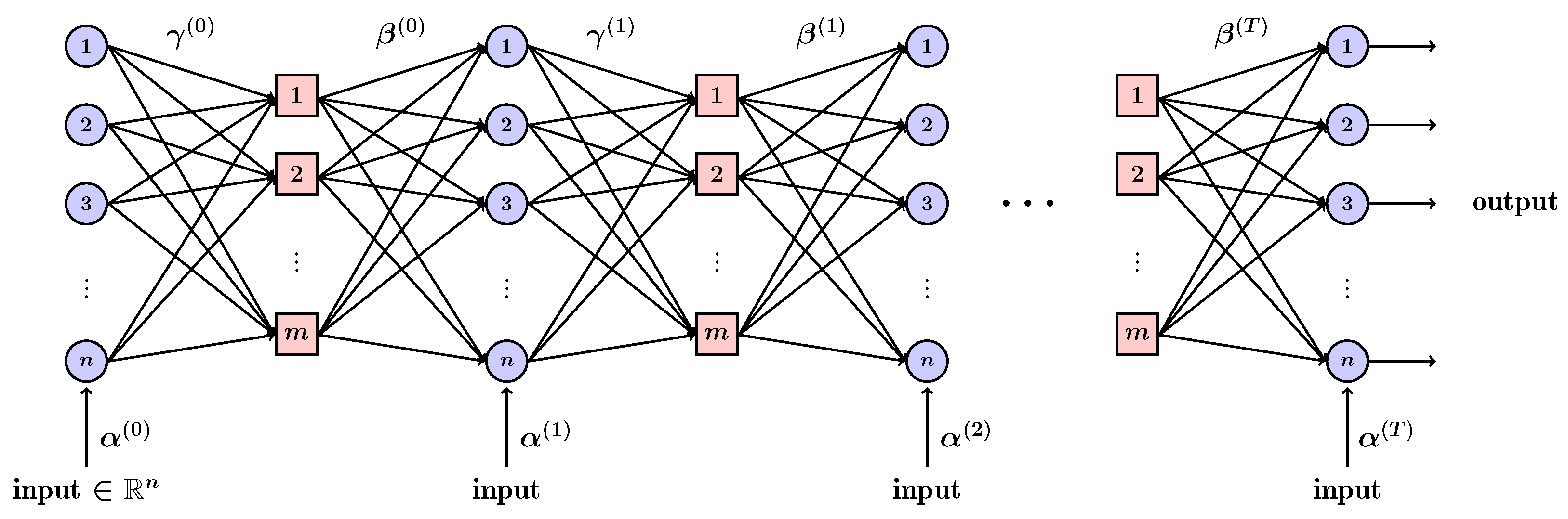
4. Weighted Belief Propagation
4.1. Parameter Sharing Schemes
4.2. WBP over
5. Adaptive Learned Message Passing Algorithms
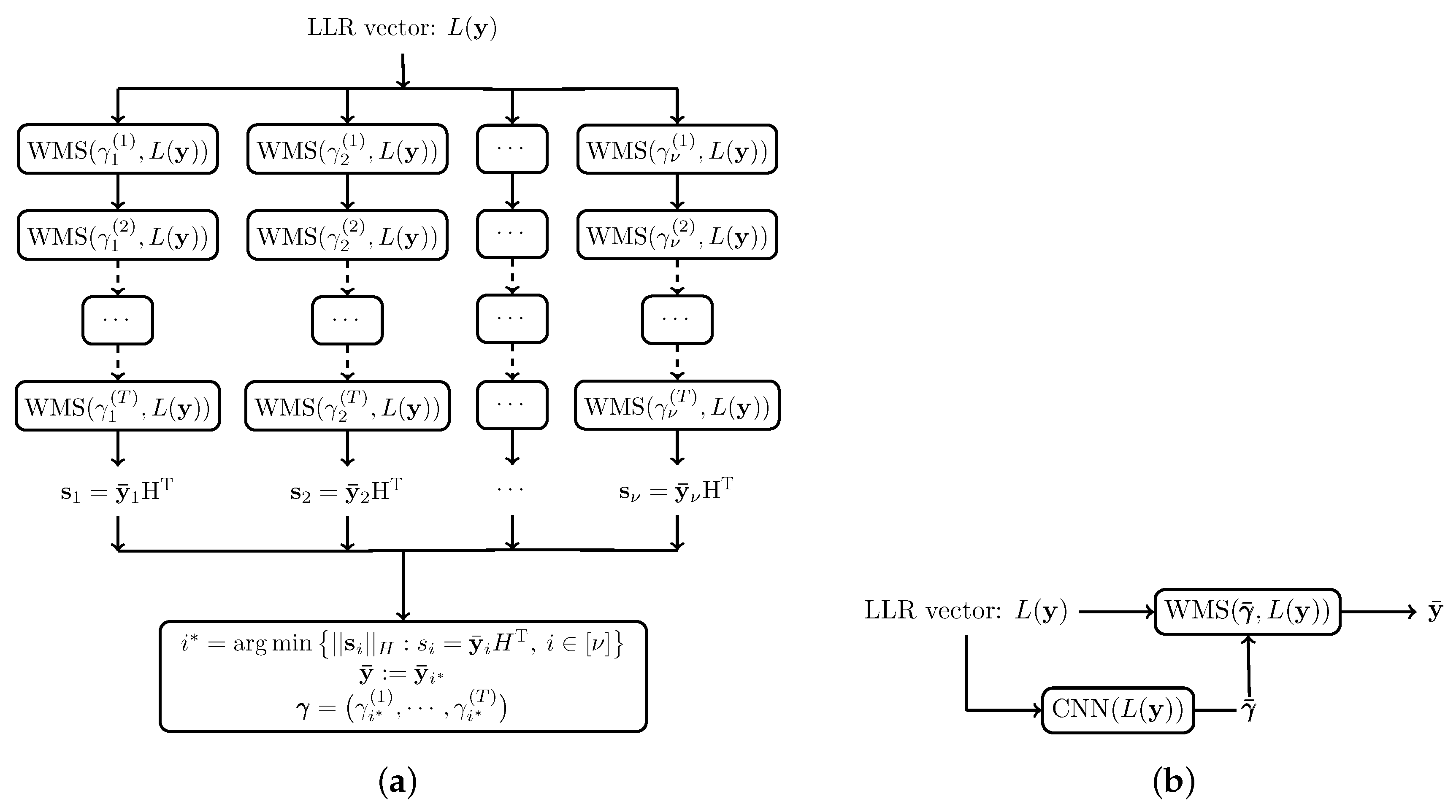
5.1. Parallel Decoders
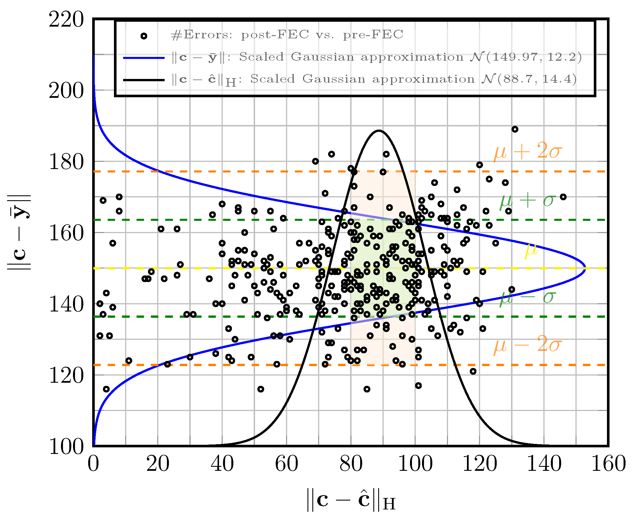
5.2. Two-Stage Decoder
6. Performance and Complexity Comparison
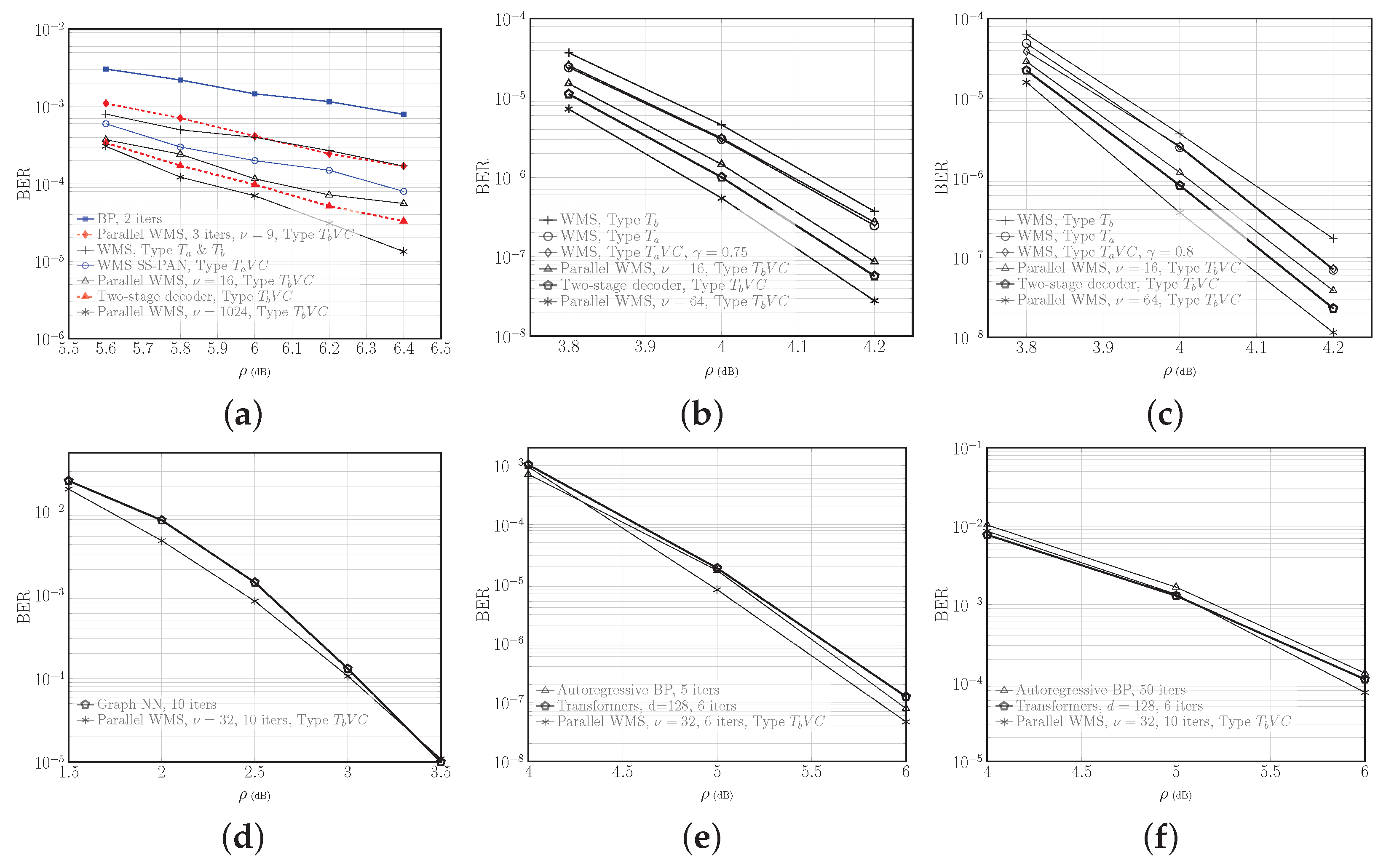
6.1. AWGN Channel
6.2. Optical Fiber Channel
7. Conclusions
Author Contributions
Funding
Institutional Review Board Statement
Data Availability Statement
Conflicts of Interest
Abbreviations
| AWGN | Additive White Gaussian Noise |
| AWEMS | Adaptive Weighted Extended Min-sum |
| AWMS | Adaptive Weighted Min-sum |
| BCH | Bose–Chaudhuri–Hocquenghem |
| BER | Bit Error Rate |
| BICD | Bit-interleaved Coded Demodulation |
| BICM | Bit-interleaved Coded Modulation |
| BP | Belief Propagation |
| CG | Coding Gain |
| CNN | Convolutional Neural Network |
| CRC | Cyclic Redundancy Check |
| DSP | Digital Signal Processing |
| EDFA | Erbium Doped Fiber Amplifier |
| EMS | Extended Min-sum |
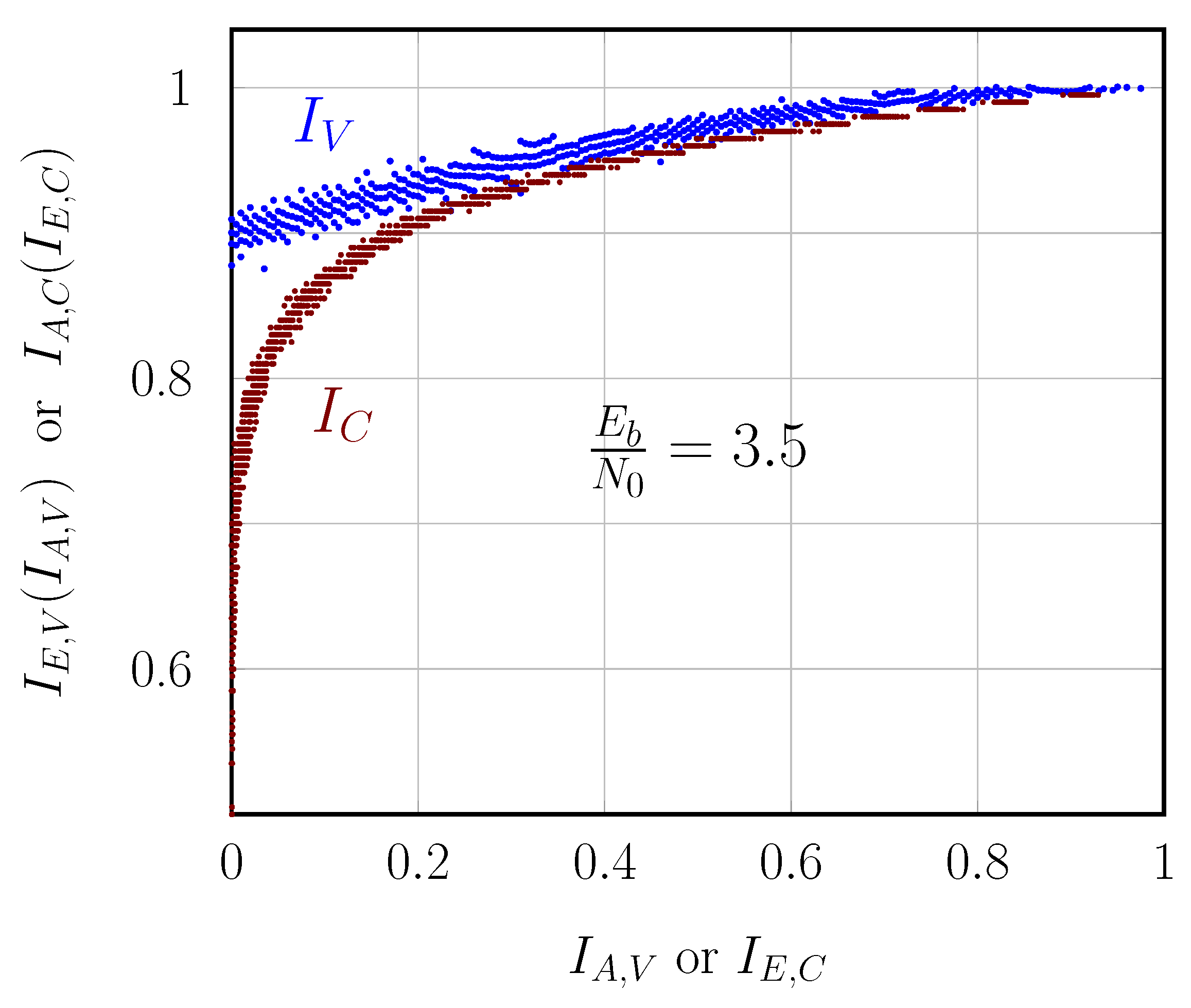
| EXIT | Extrinsic Information Transfer |
| FEC | Forward Error Correction |
| FER | Frame Error Rate |
| GF | Galois Field |
| LDPC | Low-density Parity-check |
| LLR | Log-likelihood Ratio |
| MS | Min-sum |
| NCG | Net Coding Gain |
| NF | Noise Figure |
| NN | Neural Network |
| NR | New Radio |
| NNEMS | Neural Normalized Extended Min-sum |
| NNMS | Neural Normalized Min-sum |
| OSC | Optimized Successive Cancellation |
| PB | Protograph-based |
| PCM | Parity-check Matrix |
| Probability Density Function | |
| PEG | Progressive-edge Growth |
| QAM | Quadrature Amplitude Modulation |
| QC | Quasi-cyclic |
| ReLU | Rectified Linear Unit |
| RRC | Root Raised Cosine |
| RM | Real Multiplication |
| RNN | Recurrent Neural Network |
| SC | Spatially coupled |
| SS-PAN | Simple Scaling and Parameter-adapter Networks |
| SCL | Successive Cancellation List |
| SWD | Sliding Window Decoder |
| WBP | Weighted Belief Propagation |
| WDM | Wavelength Division Multiplexing |
| WEMS | Weighted Extended Min-sum |
| WMS | Weighted Min-sum |
Appendix A. Protograph-Based QC-LDPC Codes
Appendix A.1. Construction for the Single-Edge Case
Appendix A.2. Construction for the Multi-Edge Case
Appendix A.3. Construction for Non-Binary Codes
Appendix A.4. Encoder and Decoder
Appendix B. Spatially Coupled LDPC Codes
Appendix B.1. Construction
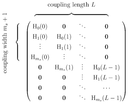 in which are block matrices, , and is obtained from as
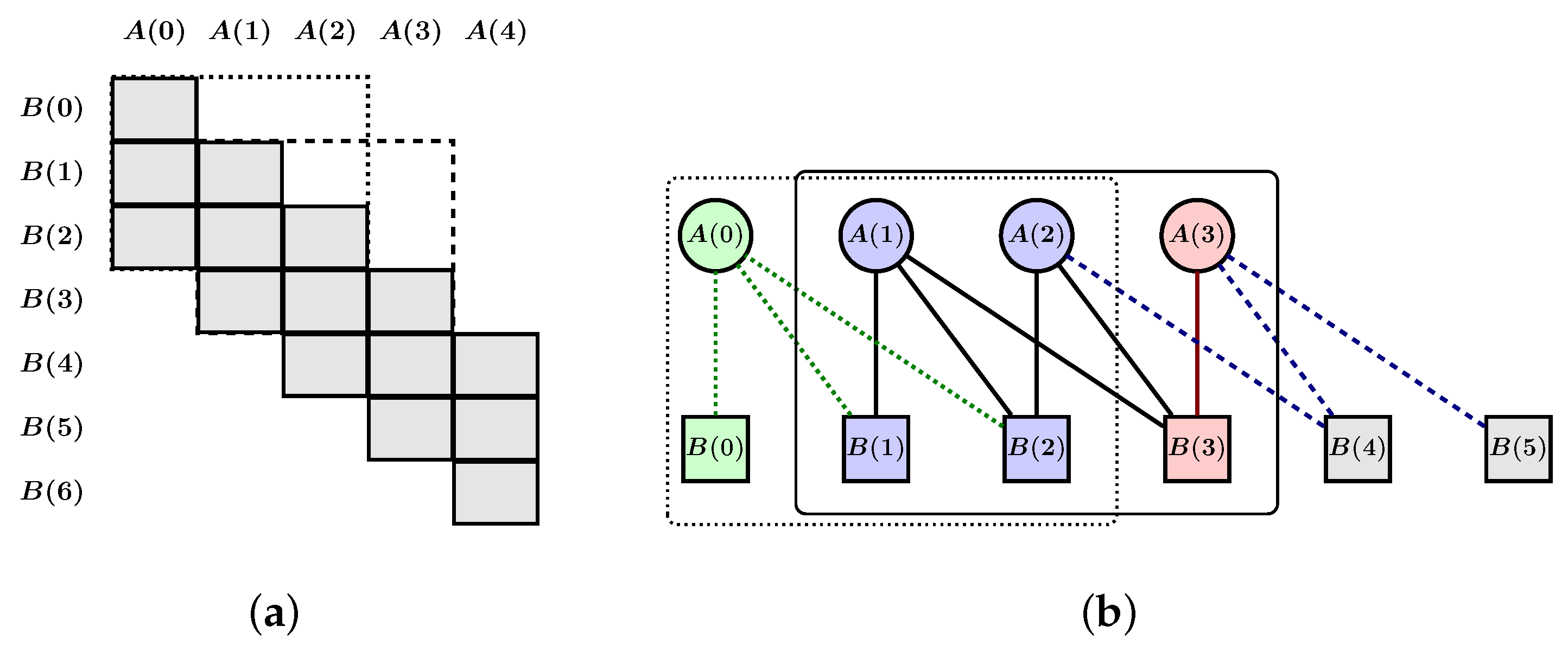
Appendix B.2. Encoder
Appendix B.3. Sliding Window Decoder
Appendix C. Parameters of Codes
References
- Pham, Q.V.; Nguyen, N.T.; Huynh-The, T.; Bao Le, L.; Lee, K.; Hwang, W.J. Intelligent radio signal processing: A survey. IEEE Access 2021, 9, 83818–83850. [Google Scholar] [CrossRef]
- Bruck, J.; Blaum, M. Neural networks, error-correcting codes, and polynomials over the binary n-cube. IEEE Trans. Inf. Theory 1989, 35, 976–987. [Google Scholar] [CrossRef]
- Zeng, G.; Hush, D.; Ahmed, N. An application of neural net in decoding error-correcting codes. In Proceedings of the 1989 IEEE International Symposium on Circuits and Systems (ISCAS), Portland, OR, USA, 8–11 May 1989; Volume 2, pp. 782–785. [Google Scholar] [CrossRef]
- Caid, W.; Means, R. Neural network error correcting decoders for block and convolutional codes. In Proceedings of the GLOBECOM ’90: IEEE Global Telecommunications Conference and Exhibition, San Diego, CA, USA, 2–5 December 1990; Volume 2, pp. 1028–1031. [Google Scholar]
- Tseng, Y.H.; Wu, J.L. Decoding Reed-Muller codes by multi-layer perceptrons. Int. J. Electron. Theor. Exp. 1993, 75, 589–594. [Google Scholar] [CrossRef]
- Marcone, G.; Zincolini, E.; Orlandi, G. An efficient neural decoder for convolutional codes. Eur. Trans. Telecommun. Relat. Technol. 1995, 6, 439–445. [Google Scholar]
- Wang, X.A.; Wicker, S. An artificial neural net Viterbi decoder. IEEE Trans. Commun. 1996, 44, 165–171. [Google Scholar] [CrossRef]
- Tallini, L.G.; Cull, P. Neural nets for decoding error-correcting codes. In Proceedings of the IEEE Technical Applications Conference and Workshops. Northcon/95. Conference Record, Portland, OR, USA, 10–12 October 1995; pp. 89–94. [Google Scholar] [CrossRef]
- Ibnkahla, M. Applications of neural networks to digital communications—A survey. Signal Process. 2000, 80, 1185–1215. [Google Scholar] [CrossRef]
- Haroon, A. Decoding of Error Correcting Codes Using Neural Networks. Ph.D. Thesis, Blekinge Institute of Technology, Blekinge, Sweden, 2012. Available online: https://www.diva-portal.org/smash/get/diva2:832503/FULLTEXT01.pdf (accessed on 11 June 2025).
- Nachmani, E.; Be’ery, Y.; Burshtein, D. Learning to decode linear codes using deep learning. In Proceedings of the 54th Annual Allerton Conference on Communication, Control, and Computing (Allerton), Monticello, IL, USA, 27–30 September 2016; pp. 341–346. [Google Scholar] [CrossRef]
- Gruber, T.; Cammerer, S.; Hoydis, J.; Brink, S.T. On deep learning-based channel decoding. In Proceedings of the 2017 51st Annual Conference on Information Sciences and Systems (CISS), Baltimore, MD, USA, 22–24 March 2017; pp. 1–6. [Google Scholar] [CrossRef]
- Kim, H.; Jiang, Y.; Rana, R.B.; Kannan, S.; Oh, S.; Viswanath, P. Communication algorithms via deep learning. In Proceedings of the International Conference on Learning Representations, Vancouver, BC, Canada, 30 April–3 May 2018; Available online: https://openreview.net/forum?id=ryazCMbR- (accessed on 11 June 2025).
- Vasić, B.; Xiao, X.; Lin, S. Learning to decode LDPC codes with finite-alphabet message passing. In Proceedings of the 2018 Information Theory and Applications Workshop (ITA), San Diego, CA, USA, 11–16 February 2018; pp. 1–9. [Google Scholar]
- Bennatan, A.; Choukroun, Y.; Kisilev, P. Deep learning for decoding of linear codes—A syndrome-based approach. In Proceedings of the 2018 IEEE International Symposium on Information Theory (ISIT), Vail, CO, USA, 17–22 June 2018; pp. 1595–1599. [Google Scholar] [CrossRef]
- Nachmani, E.; Marciano, E.; Lugosch, L.; Gross, W.J.; Burshtein, D.; Be’ery, Y. Deep learning methods for improved decoding of linear codes. IEEE J. Sel. Top. Signal Process. 2018, 12, 119–131. [Google Scholar] [CrossRef]
- Lugosch, L.P. Learning Algorithms for Error Correction. Master’s Thesis, McGill University, Montreal, QC, Canada, 2018. Available online: https://escholarship.mcgill.ca/concern/theses/c247dv63d (accessed on 11 June 2025).
- Lian, M.; Carpi, F.; Häger, C.; Pfister, H.D. Learned belief-propagation decoding with simple scaling and SNR adaptation. In Proceedings of the 2019 IEEE International Symposium on Information Theory (ISIT), Paris, France, 7–12 July 2019; pp. 161–165. [Google Scholar] [CrossRef]
- Jiang, Y.; Kannan, S.; Kim, H.; Oh, S.; Asnani, H.; Viswanath, P. DEEPTURBO: Deep Turbo decoder. In Proceedings of the 2019 IEEE 20th International Workshop on Signal Processing Advances in Wireless Communications (SPAWC), Cannes, France, 2–5 July 2019; pp. 1–5. [Google Scholar] [CrossRef]
- Carpi, F.; Häger, C.; Martalò, M.; Raheli, R.; Pfister, H.D. Reinforcement learning for channel coding: Learned bit-flipping decoding. In Proceedings of the 2019 57th Annual Allerton Conference on Communication, Control, and Computing (Allerton), Monticello, IL, USA, 24–27 September 2019; pp. 922–929. [Google Scholar] [CrossRef]
- Wang, Q.; Wang, S.; Fang, H.; Chen, L.; Chen, L.; Guo, Y. A model-driven deep learning method for normalized Min-Sum LDPC decoding. In Proceedings of the 2020 IEEE International Conference on Communications Workshops (ICC Workshops), Dublin, Ireland, 7–11 June 2020; pp. 1–6. [Google Scholar] [CrossRef]
- Huang, L.; Zhang, H.; Li, R.; Ge, Y.; Wang, J. AI coding: Learning to construct error correction codes. IEEE Trans. Commun. 2020, 68, 26–39. [Google Scholar] [CrossRef]
- Be’Ery, I.; Raviv, N.; Raviv, T.; Be’Ery, Y. Active deep decoding of linear codes. IEEE Trans. Commun. 2020, 68, 728–736. [Google Scholar] [CrossRef]
- Xu, W.; Tan, X.; Be’ery, Y.; Ueng, Y.L.; Huang, Y.; You, X.; Zhang, C. Deep learning-aided belief propagation decoder for Polar codes. IEEE J. Emerg. Sel. Top. Circuits Syst. 2020, 10, 189–203. [Google Scholar] [CrossRef]
- Buchberger, A.; Häger, C.; Pfister, H.D.; Schmalen, L.; i Amat, A.G. Pruning and quantizing neural belief propagation decoders. IEEE J. Sel. Areas Commun. 2021, 39, 1957–1966. [Google Scholar] [CrossRef]
- Dai, J.; Tan, K.; Si, Z.; Niu, K.; Chen, M.; Poor, H.V.; Cui, S. Learning to decode protograph LDPC codes. IEEE J. Sel. Areas Commun. 2021, 39, 1983–1999. [Google Scholar] [CrossRef]
- Tonnellier, T.; Hashemipour, M.; Doan, N.; Gross, W.J.; Balatsoukas-Stimming, A. Towards practical near-maximum-likelihood decoding of error-correcting codes: An overview. In Proceedings of the ICASSP 2021—2021 IEEE International Conference on Acoustics, Speech and Signal Processing (ICASSP), Toronto, ON, Canada, 6–11 June 2021; pp. 8283–8287. [Google Scholar] [CrossRef]
- Wang, L.; Chen, S.; Nguyen, J.; Dariush, D.; Wesel, R. Neural-network-optimized degree-specific weights for LDPC MinSum decoding. In Proceedings of the 2021 11th International Symposium on Topics in Coding (ISTC), Montreal, QC, Canada, 30 August–3 September 2021; pp. 1–5. [Google Scholar] [CrossRef]
- Habib, S.; Beemer, A.; Kliewer, J. Belief propagation decoding of short graph-based channel codes via reinforcement learning. IEEE J. Sel. Areas Inf. Theory 2021, 2, 627–640. [Google Scholar] [CrossRef]
- Nachmani, E.; Wolf, L. Autoregressive belief propagation for decoding block codes. arXiv 2021, arXiv:2103.11780. [Google Scholar]
- Nachmani, E.; Be’ery, Y. Neural decoding with optimization of node activations. IEEE Commun. Lett. 2022, 26, 2527–2531. [Google Scholar] [CrossRef]
- Cammerer, S.; Ait Aoudia, F.; Dörner, S.; Stark, M.; Hoydis, J.; Ten Brink, S. Trainable communication systems: Concepts and prototype. IEEE Trans. Commun. 2020, 68, 5489–5503. [Google Scholar] [CrossRef]
- Cammerer, S.; Hoydis, J.; Aoudia, F.A.; Keller, A. Graph neural networks for channel decoding. In Proceedings of the 2022 IEEE Globecom Workshops (GC Wkshps), Rio de Janeiro, Brazil, 4–8 December 2022; pp. 486–491. [Google Scholar] [CrossRef]
- Choukroun, Y.; Wolf, L. Error correction code transformer. Conf. Neural Inf. Proc. Syst. 2022, 35, 38695–38705. Available online: https://proceedings.neurips.cc/paper_files/paper/2022/file/fcd3909db30887ce1da519c4468db668-Paper-Conference.pdf (accessed on 11 June 2025).
- Jamali, M.V.; Saber, H.; Hatami, H.; Bae, J.H. ProductAE: Toward training larger channel codes based on neural product codes. In Proceedings of the ICC 2022—IEEE International Conference on Communications, Seoul, Republic of Korea, 16–20 May 2022; pp. 3898–3903. [Google Scholar] [CrossRef]
- Dörner, S.; Clausius, J.; Cammerer, S.; ten Brink, S. Learning joint detection, equalization and decoding for short-packet communications. IEEE Trans. Commun. 2022, 71, 837–850. [Google Scholar] [CrossRef]
- Li, G.; Yu, X.; Luo, Y.; Wei, G. A bottom-up design methodology of neural Min-Sum decoders for LDPC codes. IET Commun. 2023, 17, 377–386. [Google Scholar] [CrossRef]
- Wang, Q.; Liu, Q.; Wang, S.; Chen, L.; Fang, H.; Chen, L.; Guo, Y.; Wu, Z. Normalized Min-Sum neural network for LDPC decoding. IEEE Trans. Cogn. Commun. Netw. 2023, 9, 70–81. [Google Scholar] [CrossRef]
- Wang, L.; Terrill, C.; Divsalar, D.; Wesel, R. LDPC decoding with degree-specific neural message weights and RCQ decoding. IEEE Trans. Commun. 2023, 72, 1912–1924. [Google Scholar] [CrossRef]
- Clausius, J.; Geiselhart, M.; Ten Brink, S. Component training of Turbo Autoencoders. In Proceedings of the 2023 12th International Symposium on Topics in Coding (ISTC), Brest, France, 4–8 September 2023; pp. 1–5. [Google Scholar] [CrossRef]
- Choukroun, Y.; Wolf, L. A foundation model for error correction codes. In Proceedings of the International Conference on Learning Representations, Vienna, Austria, 7–11 May 2024; Available online: https://openreview.net/forum?id=7KDuQPrAF3 (accessed on 15 March 2012).
- Choukroun, Y.; Wolf, L. Learning linear block error correction codes. arXiv 2024, arXiv:2405.04050. [Google Scholar]
- Clausius, J.; Geiselhart, M.; Tandler, D.; Brink, S.T. Graph neural network-based joint equalization and decoding. In Proceedings of the 2024 IEEE International Symposium on Information Theory (ISIT), Athens, Greece, 7–12 July 2024; pp. 1203–1208. [Google Scholar] [CrossRef]
- Adiga, S.; Xiao, X.; Tandon, R.; Vasić, B.; Bose, T. Generalization bounds for neural belief propagation decoders. IEEE Trans. Inf. Theory 2024, 70, 4280–4296. [Google Scholar] [CrossRef]
- Kim, T.; Sung Park, J. Neural self-corrected Min-Sum decoder for NR LDPC codes. IEEE Commun. Lett. 2024, 28, 1504–1508. [Google Scholar] [CrossRef]
- Ninkovic, V.; Kundacina, O.; Vukobratovic, D.; Häger, C.; i Amat, A.G. Decoding Quantum LDPC Codes Using Graph Neural Networks. In Proceedings of the GLOBECOM 2024—2024 IEEE Global Communications Conference, Cape Town, South Africa, 8–12 December 2024; pp. 3479–3484. [Google Scholar]
- Cammerer, S.; Gruber, T.; Hoydis, J.; Ten Brink, S. Scaling deep learning-based decoding of Polar codes via partitioning. In Proceedings of the GLOBECOM 2017—2017 IEEE Global Communications Conference, Singapore, 4–8 December 2017; pp. 1–6. [Google Scholar] [CrossRef]
- Sagar, V.; Jacyna, G.M.; Szu, H. Block-parallel decoding of convolutional codes using neural network decoders. Neurocomputing 1994, 6, 455–471. [Google Scholar] [CrossRef]
- Hussain, M.; Bedi, J.S. Reed-Solomon encoder/decoder application using a neural network. Proc. SPIE 1991, 1469, 463–471. [Google Scholar] [CrossRef]
- Alston, M.D.; Chau, P.M. A neural network architecture for the decoding of long constraint length convolutional codes. In Proceedings of the 1990 IJCNN International Joint Conference on Neural Networks, San Diego, CA, USA, 17–21 June 1990; pp. 121–126. [Google Scholar] [CrossRef]
- Wu, X.; Jiang, M.; Zhao, C. Decoding optimization for 5G LDPC codes by machine learning. IEEE Access 2018, 6, 50179–50186. [Google Scholar] [CrossRef]
- Miloslavskaya, V.; Li, Y.; Vucetic, B. Neural network-based adaptive Polar coding. IEEE Trans. Commun. 2024, 72, 1881–1894. [Google Scholar] [CrossRef]
- Doan, N.; Hashemi, S.A.; Mambou, E.N.; Tonnellier, T.; Gross, W.J. Neural belief propagation decoding of CRC-polar concatenated codes. In Proceedings of the ICC 2019—2019 IEEE International Conference on Communications (ICC), Shanghai, China, 20–24 May 2019; pp. 1–6. [Google Scholar]
- Yang, C.; Zhou, Y.; Si, Z.; Dai, J. Learning to decode protograph LDPC codes over fadings with imperfect CSIs. In Proceedings of the 2023 IEEE Wireless Communications and Networking Conference (WCNC), Glasgow, UK, 26–29 March 2023; pp. 1–6. [Google Scholar] [CrossRef]
- Wang, M.; Li, Y.; Liu, J.; Guo, T.; Wu, H.; Lau, F.C. Neural layered min-sum decoders for cyclic codes. Phys. Commun. 2023, 61, 102194. [Google Scholar] [CrossRef]
- Raviv, T.; Goldman, A.; Vayner, O.; Be’ery, Y.; Shlezinger, N. CRC-aided learned ensembles of belief-propagation polar decoders. In Proceedings of the ICASSP 2024—2024 IEEE International Conference on Acoustics, Speech and Signal Processing (ICASSP), Seoul, Republic of Korea, 14–19 April 2024; pp. 8856–8860. [Google Scholar]
- Raviv, T.; Raviv, N.; Be’ery, Y. Data-driven ensembles for deep and hard-decision hybrid decoding. In Proceedings of the 2020 IEEE International Symposium on Information Theory (ISIT), Los Angeles, CA, USA, 21–26 June 2020; pp. 321–326. [Google Scholar] [CrossRef]
- Kwak, H.Y.; Yun, D.Y.; Kim, Y.; Kim, S.H.; No, J.S. Boosting learning for LDPC codes to improve the error-floor performance. In Proceedings of the 37th Conference on Neural Information Processing Systems (NeurIPS 2023), New Orleans, LA, USA, 10–16 December 2023; Volume 36, pp. 22115–22131. Available online: https://proceedings.neurips.cc/paper_files/paper/2023/file/463a91da3c832bd28912cd0d1b8d9974-Paper-Conference.pdf (accessed on 11 June 2025).
- Schmalen, L.; Suikat, D.; Rösener, D.; Aref, V.; Leven, A.; ten Brink, S. Spatially coupled codes and optical fiber communications: An ideal match? In Proceedings of the 2015 IEEE 16th International Workshop on Signal Processing Advances in Wireless Communications (SPAWC), Stockholm, Sweden, 28 June–1 July 2015; pp. 460–464. [Google Scholar] [CrossRef]
- Kudekar, S.; Richardson, T.; Urbanke, R.L. Spatially coupled ensembles universally achieve capacity under belief propagation. IEEE Trans. Inf. Theory 2013, 59, 7761–7813. [Google Scholar] [CrossRef]
- Liga, G.; Alvarado, A.; Agrell, E.; Bayvel, P. Information rates of next-generation long-haul optical fiber systems using coded modulation. IEEE J. Lightw. Technol. 2017, 35, 113–123. [Google Scholar] [CrossRef]
- Feltstrom, A.J.; Truhachev, D.; Lentmaier, M.; Zigangirov, K.S. Braided block codes. IEEE Trans. Inf. Theory 2009, 55, 2640–2658. [Google Scholar] [CrossRef]
- Montorsi, G.; Benedetto, S. Design of spatially coupled Turbo product codes for optical communications. In Proceedings of the 2021 11th International Symposium on Topics in Coding (ISTC), Montreal, QC, Canada, 30 August–3 September 2021; pp. 1–5. [Google Scholar] [CrossRef]
- Smith, B.P.; Farhood, A.; Hunt, A.; Kschischang, F.R.; Lodge, J. Staircase codes: FEC for 100 Gb/s OTN. IEEE J. Lightw. Technol. 2012, 30, 110–117. [Google Scholar] [CrossRef]
- Zhang, L.M.; Kschischang, F.R. Staircase codes with 6% to 33% overhead. IEEE J. Lightw. Technol. 2014, 32, 1999–2002. [Google Scholar] [CrossRef]
- Zhang, L. Analysis and Design of Staircase Codes for High Bit-Rate Fibre-Optic Communication. Ph.D. Thesis, University of Toronto, Toronto, ON, Canada, 2017. Available online: https://tspace.library.utoronto.ca/bitstream/1807/79549/3/Zhang_Lei_201706_PhD_thesis.pdf (accessed on 11 June 2025).
- Shehadeh, M.; Kschischang, F.R.; Sukmadji, A.Y. Generalized staircase codes with arbitrary bit degree. In Proceedings of the 2024 Optical Fiber Communications Conference and Exhibition (OFC), San Diego, CA, USA, 24–28 March 2024; pp. 1–3. Available online: https://ieeexplore.ieee.org/abstract/document/10526860 (accessed on 11 June 2025).
- Sukmadji, A.Y.; Martínez-Peñas, U.; Kschischang, F.R. Zipper codes. IEEE J. Lightw. Technol. 2022, 40, 6397–6407. [Google Scholar] [CrossRef]
- Ryan, W.; Lin, S. Channel Codes: Classical and Modern; Cambridge University Press: Cambridge, UK, 2009; Available online: https://www.cambridge.org/fr/universitypress/subjects/engineering/communications-and-signal-processing/channel-codes-classical-and-modern?format=HB&isbn=9780521848688 (accessed on 11 June 2025).
- Ahmad, T. Polar Codes for Optical Communications. Ph.D. Thesis, Bilkent University, Ankara, Turkey, 2016. Available online: https://api.semanticscholar.org/CorpusID:116423770 (accessed on 11 June 2025).
- Barakatain, M.; Kschischang, F.R. Low-complexity concatenated LDPC-staircase codes. IEEE J. Lightw. Technol. 2018, 36, 2443–2449. [Google Scholar] [CrossRef]
- i Amat, A.G.; Liva, G.; Steiner, F. Coding for optical communications—Can we approach the Shannon limit with low complexity? In Proceedings of the 45th European Conference on Optical Communication (ECOC 2019), Dublin, Ireland, 22–26 September 2019; pp. 1–4. [Google Scholar] [CrossRef]
- Zhang, L.M.; Kschischang, F.R. Low-complexity soft-decision concatenated LDGM-staircase FEC for high-bit-rate fiber-optic communication. IEEE J. Lightw. Technol. 2017, 35, 3991–3999. [Google Scholar] [CrossRef]
- Agrawal, G.P. Nonlinear Fiber Optics, 6th ed.; Academic Press: San Francisco, CA, USA, 2019. [Google Scholar]
- Kramer, G.; Yousefi, M.I.; Kschischang, F. Upper bound on the capacity of a cascade of nonlinear and noisy channels. arXiv 2015, arXiv:1503.07652, 1–4. [Google Scholar]
- Secondini, M.; Rommel, S.; Meloni, G.; Fresi, F.; Forestieri, E.; Poti, L. Single-step digital backpropagation for nonlinearity mitigation. Photonic Netw. Commun. 2016, 31, 493–502. [Google Scholar] [CrossRef]
- Union, I.T. G.709: Interface for the Optical Transport Network (OTN). 2020. Available online: https://www.itu.int/rec/T-REC-G.709/ (accessed on 11 June 2025).
- Polyanskiy, Y.; Poor, H.V.; Verdu, S. Channel coding rate in the finite blocklength regime. IEEE Trans. Inf. Theory 2010, 56, 2307–2359. [Google Scholar] [CrossRef]
- Mezard, M.; Montanari, A. Information, Physics, and Computation; Oxford University Press: Oxford, UK, 2009. [Google Scholar]
- Dolecek, L.; Divsalar, D.; Sun, Y.; Amiri, B. Non-binary protograph-based LDPC codes: Enumerators, analysis, and designs. IEEE Trans. Inf. Theory 2014, 60, 3913–3941. [Google Scholar] [CrossRef]
- Boutillon, E.; Conde-Canencia, L.; Al Ghouwayel, A. Design of a GF(64)-LDPC decoder based on the EMS algorithm. IEEE Trans. Circ. Syst. I 2013, 60, 2644–2656. [Google Scholar] [CrossRef]
- Liang, Y.; Lam, C.T.; Wu, Q.; Ng, B.K.; Im, S.K. A model-driven deep learning-based non-binary LDPC decoding algorithm. TechRxiv 2024. [Google Scholar] [CrossRef]
- Fu, Y.; Zhu, X.; Li, B. A survey on instance selection for active learning. Knowl. Inf. Syst. 2013, 35, 249–283. [Google Scholar] [CrossRef]
- Noghrei, H.; Sadeghi, M.R.; Mow, W.H. Efficient active deep decoding of linear codes using importance sampling. IEEE Commun. Lett. 2024. [Google Scholar] [CrossRef]
- Helmling, M.; Scholl, S.; Gensheimer, F.; Dietz, T.; Kraft, K.; Ruzika, S.; Wehn, N. Database of Channel Codes and ML Simulation Results. 2024. Available online: https://rptu.de/channel-codes/ml-simulation-results (accessed on 11 June 2025).
- Hu, X.Y.; Eleftheriou, E.; Arnold, D.M. Progressive edge-growth Tanner graphs. In Proceedings of the GLOBECOM’01. IEEE Global Telecommunications Conference (Cat. No.01CH37270), San Antonio, TX, USA, 25–29 November 2001; Volume 2, pp. 995–1001. [Google Scholar] [CrossRef]
- Tasdighi, A.; Yousefi, M. The Repository for the Papers on the Adaptive Weighted Belief Propagation. 2025. Available online: https://github.com/comsys2/adaptive-wbp (accessed on 11 June 2025).
- Tal, I.; Vardy, A. List decoding of Polar codes. IEEE Trans. Inf. Theory 2015, 61, 2213–2226. [Google Scholar] [CrossRef]
- Süral, A.; Sezer, E.G.; Kolağasıoğlu, E.; Derudder, V.; Bertrand, K. Tb/s Polar successive cancellation decoder 16 nm ASIC implementation. arXiv 2020, arXiv:2009.09388. [Google Scholar]
- Cassagne, A.; Hartmann, O.; Léonardon, M.; He, K.; Leroux, C.; Tajan, R.; Aumage, O.; Barthou, D.; Tonnellier, T.; Pignoly, V.; et al. AFF3CT: A fast forward error correction toolbox. SoftwareX 2019, 10, 100345. [Google Scholar] [CrossRef]
- Tang, Y.; Zhou, L.; Zhang, S.; Chen, C. Normalized Neural Network for Belief Propagation LDPC Decoding. In Proceedings of the 2021 IEEE International Conference on Networking, Sensing and Control (ICNSC), Xiamen, China, 3–5 December 2021. [Google Scholar]
- Tazoe, K.; Kasai, K.; Sakaniwa, K. Efficient termination of spatially-coupled codes. In Proceedings of the 2012 IEEE Information Theory Workshop, Lausanne, Switzerland, 3–7 September 2012; pp. 30–34. [Google Scholar] [CrossRef]
- Takasu, T. PocketSDR. 2024. Available online: https://github.com/tomojitakasu/PocketSDR/tree/master/python (accessed on 11 June 2025).
- Li, Z.; Kumar, B.V. A class of good quasi-cyclic low-density parity check codes based on progressive edge growth graph. In Proceedings of the Conference Record of the Thirty-Eighth Asilomar Conference on Signals, Systems and Computers, Pacific Grove, CA, USA, 7–10 November 2004; Volume 2, pp. 1990–1994. [Google Scholar] [CrossRef]
- Tasdighi, A.; Boutillon, E. Integer ring sieve for constructing compact QC-LDPC codes with girths 8, 10, and 12. IEEE Trans. Inf. Theory 2022, 68, 35–46. [Google Scholar] [CrossRef]
- Li, Z.; Chen, L.; Zeng, L.; Lin, S.; Fong, W. Efficient encoding of quasi-cyclic low-density parity-check codes. IEEE Trans. Commun. 2006, 54, 71–81. [Google Scholar] [CrossRef]
- Mitchell, D.G.; Rosnes, E. Edge spreading design of high rate array-based SC-LDPC codes. In Proceedings of the 2017 IEEE International Symposium on Information Theory (ISIT), Aachen, Germany, 25–30 June 2017; pp. 2940–2944. [Google Scholar] [CrossRef]
- Lentmaier, M.; Prenda, M.M.; Fettweis, G.P. Efficient message passing scheduling for terminated LDPC convolutional codes. In Proceedings of the 2011 IEEE International Symposium on Information Theory Proceedings, St. Petersburg, Russia, 31 July–5 August 2011; pp. 1826–1830. [Google Scholar] [CrossRef]
- Ali, I.; Kim, J.H.; Kim, S.H.; Kwak, H.; No, J.S. Improving windowed decoding of SC LDPC codes by effective decoding termination, message reuse, and amplification. IEEE Access 2018, 6, 9336–9346. [Google Scholar] [CrossRef]
- Land, I. Code Design with EXIT Charts. 2013. Available online: https://api.semanticscholar.org/CorpusID:61966354 (accessed on 11 June 2025).
- Koike-Akino, T.; Millar, D.S.; Kojima, K.; Parsons, K. Stochastic EXIT design for low-latency short-block LDPC codes. In Proceedings of the 2020 Optical Fiber Communications Conference and Exhibition (OFC), San Diego, CA, USA, 8–12 March 2020; pp. 1–3. Available online: https://ieeexplore.ieee.org/document/9083080 (accessed on 11 June 2025).

| AWGN Channel | |
|---|---|
| Low rate | High rate |
| BCH , | QC-LDPC , |
| QC-LDPC , | QC-LDPC , |
| QC-LDPC , | QC-LDPC , |
| Irregular LDPC , | Polar , |
| Irregular LDPC , | |
| Optical Fiber Channel | |
| Inner code | Outer code |
| Single-edge QC-LDPC , | Multi-edge QC-LDPC , |
| Non-binary multi-edge | |
| Parameter Name | Value |
|---|---|
| Transmitter parameters | |
| WDM channels | 5 |
| Symbol rate | 32 Gbaud |
| RRC roll-off | 0.01 |
| Channel frequency spacing | 33 GHz |
| Fiber channel parameters | |
| Attenuation | 0.2 dB/km |
| Dispersion parameter (D) | 17 ps/nm/km |
| Nonlinearity parameter | 1.2 l/(W·km) |
| Span configuration | 8 × 80 km |
| EDFA gain | 16 dB |
| EDFA noise figure | 5 dB |
| Code | |||
|---|---|---|---|
| – | – |
| Average RM per Iteration | |||||
|---|---|---|---|---|---|
| No weight sharing | |||||
| WMS [16] | 1 | 768 | 25,792 | 40,160 | |
| Weight sharing | |||||
| WMS, Type | 1 | 768 | 25,792 | 40,160 | |
| WMS, Type | 1 | 63 | 3226 | 4016 | |
| Parallel WMS Type , | 1 | 1440 | 77,376 | 84,336 | |
| Parallel WMS Type , | 1 | – | ≃ | ≃ | |
| Parallel WMS Type , | 1 | 92,340 | – | – | |
| Two-stage decoder Type , | 1 | ≃300 | ≃14,093 | ≃17,558 | |
| WMS SS−PAN, Type [18] | 1 | 153 | 8060 | 9287 | |
| Inner-SD Decoder | Inner | Total | NCG Inner | NCG Total | Inner | Total | Inner | Total | |
|---|---|---|---|---|---|---|---|---|---|
| AWMS | |||||||||
| NNMS | |||||||||
| MS | |||||||||
| AWMS | |||||||||
| NNMS | |||||||||
| MS |
| Inner-SD Decoder | Inner | Total | NCG Inner | NCG Total | Inner | Total | Inner | Total | |
|---|---|---|---|---|---|---|---|---|---|
| AWEMS | |||||||||
| NNEMS | |||||||||
| EMS | 2 | ||||||||
| AWEMS | |||||||||
| NNEMS | |||||||||
| EMS |
Disclaimer/Publisher’s Note: The statements, opinions and data contained in all publications are solely those of the individual author(s) and contributor(s) and not of MDPI and/or the editor(s). MDPI and/or the editor(s) disclaim responsibility for any injury to people or property resulting from any ideas, methods, instructions or products referred to in the content. |
© 2025 by the authors. Licensee MDPI, Basel, Switzerland. This article is an open access article distributed under the terms and conditions of the Creative Commons Attribution (CC BY) license (https://creativecommons.org/licenses/by/4.0/).
Share and Cite
Tasdighi, A.; Yousefi, M. Adaptive Learned Belief Propagation for Decoding Error-Correcting Codes. Entropy 2025, 27, 795. https://doi.org/10.3390/e27080795
Tasdighi A, Yousefi M. Adaptive Learned Belief Propagation for Decoding Error-Correcting Codes. Entropy. 2025; 27(8):795. https://doi.org/10.3390/e27080795
Chicago/Turabian StyleTasdighi, Alireza, and Mansoor Yousefi. 2025. "Adaptive Learned Belief Propagation for Decoding Error-Correcting Codes" Entropy 27, no. 8: 795. https://doi.org/10.3390/e27080795
APA StyleTasdighi, A., & Yousefi, M. (2025). Adaptive Learned Belief Propagation for Decoding Error-Correcting Codes. Entropy, 27(8), 795. https://doi.org/10.3390/e27080795