
Description Generation Using Variational Auto-Encoders for Precursor microRNA


Abstract
1. Introduction
2. Methods
2.1. Data
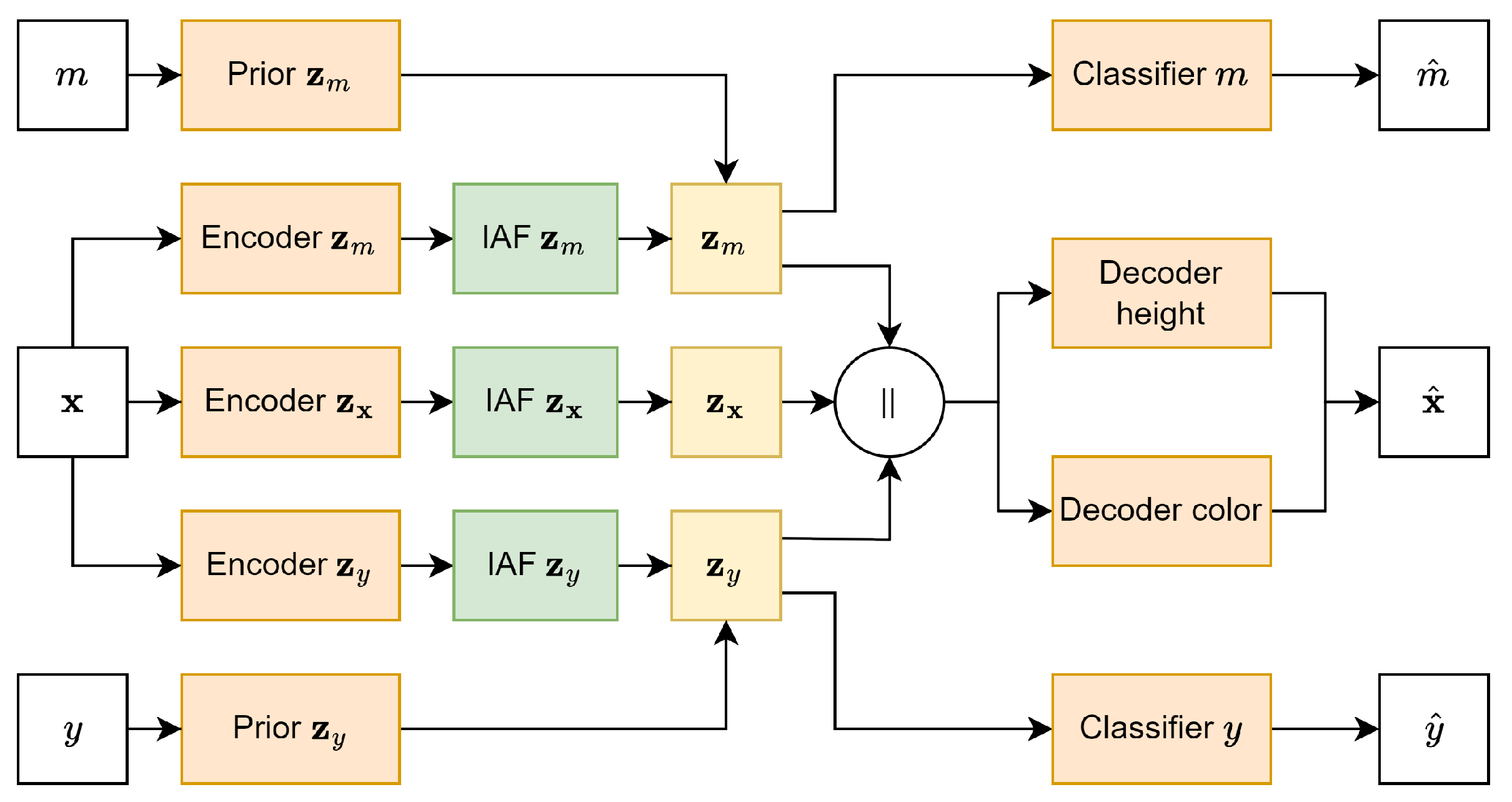
2.2. Model
2.3. Decision Tree
| Algorithm 1 MakeSplit() |
|
3. Results
3.1. Performance
3.2. Conditional Generation
3.3. Decision Tree
4. Discussion
Author Contributions
Funding
Data Availability Statement
Conflicts of Interest
Abbreviations
| VAE | Variational Auto-Encoder |
| RNA | Ribonucleic Acid |
| KL | Kullback–Leibler |
| DIVA | Domain Independent Variational Auto-encoder |
| DT | Decision Tree |
References
- Alles, J.; Fehlmann, T.; Fischer, U.; Backes, C.; Galata, V.; Minet, M.; Hart, M.; Abu-Halima, M.; Grässer, F.A.; Lenhof, H.P.; et al. An estimate of the total number of true human miRNAs. Nucleic Acids Res. 2019, 47, 3353–3364. [Google Scholar] [CrossRef] [PubMed]
- Kozomara, A.; Birgaoanu, M.; Griffiths-Jones, S. miRBase: From microRNA sequences to function. Nucleic Acids Res. 2019, 47, D155–D162. [Google Scholar] [CrossRef]
- Ng, K.L.S.; Mishra, S.K. De novo SVM classification of precursor microRNAs from genomic pseudo hairpins using global and intrinsic folding measures. Bioinformatics 2007, 23, 1321–1330. [Google Scholar] [CrossRef]
- Saçar, M.D.; Allmer, J. Machine learning methods for microRNA gene prediction. In miRNomics: microRNA Biology and Computational Analysis; Springer: Berlin/Heidelberg, Germany, 2014; pp. 177–187. [Google Scholar]
- Erson-Bensan, A.E. Introduction to microRNAs in biological systems. In miRNomics: microRNA Biology and Computational Analysis; Springer: Berlin/Heidelberg, Germany, 2014; pp. 1–14. [Google Scholar]
- Allmer, J. Computational and bioinformatics methods for microRNA gene prediction. In miRNomics: microRNA Biology and Computational Analysis; Springer: Berlin/Heidelberg, Germany, 2014; pp. 157–175. [Google Scholar]
- Saçar Demirci, M.D.; Baumbach, J.; Allmer, J. On the performance of pre-microRNA detection algorithms. Nat. Commun. 2017, 8, 330. [Google Scholar] [CrossRef]
- Jiang, P.; Wu, H.; Wang, W.; Ma, W.; Sun, X.; Lu, Z. MiPred: Classification of real and pseudo microRNA precursors using random forest prediction model with combined features. Nucleic Acids Res. 2007, 35, W339–W344. [Google Scholar] [CrossRef]
- Batuwita, R.; Palade, V. microPred: Effective classification of pre-miRNAs for human miRNA gene prediction. Bioinformatics 2009, 25, 989–995. [Google Scholar] [CrossRef]
- Ding, J.; Zhou, S.; Guan, J. MiRenSVM: Towards better prediction of microRNA precursors using an ensemble SVM classifier with multi-loop features. BMC Bioinform. 2010, 11, S11. [Google Scholar] [CrossRef]
- Xue, C.; Li, F.; He, T.; Liu, G.P.; Li, Y.; Zhang, X. Classification of real and pseudo microRNA precursors using local structure-sequence features and support vector machine. BMC Bioinform. 2005, 6, 310. [Google Scholar] [CrossRef]
- Cordero, J.; Menkovski, V.; Allmer, J. Detection of pre-microRNA with Convolutional Neural Networks. BioRxiv 2019. [Google Scholar] [CrossRef]
- Do, B.T.; Golkov, V.; Gürel, G.E.; Cremers, D. Precursor microRNA identification using deep convolutional neural networks. BioRxiv 2018. [Google Scholar] [CrossRef]
- Tasdelen, A.; Sen, B. A hybrid CNN-LSTM model for pre-miRNA classification. Sci. Rep. 2021, 11, 14125. [Google Scholar] [CrossRef] [PubMed]
- Zheng, X.; Xu, S.; Zhang, Y.; Huang, X. Nucleotide-level convolutional neural networks for pre-miRNA classification. Sci. Rep. 2019, 9, 628. [Google Scholar] [CrossRef] [PubMed]
- Yones, C.; Raad, J.; Bugnon, L.A.; Milone, D.H.; Stegmayer, G. High precision in microRNA prediction: A novel genome-wide approach with convolutional deep residual networks. Comput. Biol. Med. 2021, 134, 104448. [Google Scholar] [CrossRef] [PubMed]
- Bugnon, L.A.; Raad, J.; Merino, G.A.; Yones, C.; Ariel, F.; Milone, D.H.; Stegmayer, G. Deep Learning for the discovery of new pre-miRNAs: Helping the fight against COVID-19. Mach. Learn. Appl. 2021, 6, 100150. [Google Scholar] [CrossRef] [PubMed]
- Park, S.; Min, S.; Choi, H.S.; Yoon, S. Deep recurrent neural network-based identification of precursor micrornas. In Proceedings of the Advances in Neural Information Processing Systems, Long Beach, CA, USA, 4–9 December 2017; Volume 30. [Google Scholar]
- Bell, J.; Hendrix, D.A. Predicting Drosha and Dicer Cleavage Sites with DeepMirCut. Front. Mol. Biosci. 2022, 8, 799056. [Google Scholar] [CrossRef]
- Raad, J.; Bugnon, L.A.; Milone, D.H.; Stegmayer, G. miRe2e: A full end-to-end deep model based on transformers for prediction of pre-miRNAs. Bioinformatics 2022, 38, 1191–1197. [Google Scholar] [CrossRef]
- Gupta, S.; Shankar, R. miWords: Transformer-based composite deep learning for highly accurate discovery of pre-miRNA regions across plant genomes. Briefings Bioinform. 2023, 24, bbad088. [Google Scholar] [CrossRef]
- Van den Brandt, I. Towards Concept-Based Interpretability of Pre-miRNA Detection Using Convolutional Neural Networks. Master’s Thesis, Eindhoven University of Technology, Eindhoven, The Netherlands, 2021. [Google Scholar]
- Ingraham, J.; Garg, V.; Barzilay, R.; Jaakkola, T. Generative models for graph-based protein design. In Proceedings of the Advances in Neural Information Processing Systems, Vancouver, BC, Canada, 8–14 December 2019; Volume 32. [Google Scholar]
- Strokach, A.; Kim, P.M. Deep generative modeling for protein design. Curr. Opin. Struct. Biol. 2022, 72, 226–236. [Google Scholar] [CrossRef]
- Cheng, Y.; Gong, Y.; Liu, Y.; Song, B.; Zou, Q. Molecular design in drug discovery: A comprehensive review of deep generative models. Briefings Bioinform. 2021, 22, bbab344. [Google Scholar] [CrossRef]
- Grisoni, F.; Huisman, B.J.; Button, A.L.; Moret, M.; Atz, K.; Merk, D.; Schneider, G. Combining generative artificial intelligence and on-chip synthesis for de novo drug design. Sci. Adv. 2021, 7, eabg3338. [Google Scholar] [CrossRef]
- Tong, X.; Liu, X.; Tan, X.; Li, X.; Jiang, J.; Xiong, Z.; Xu, T.; Jiang, H.; Qiao, N.; Zheng, M. Generative models for de novo drug design. J. Med. Chem. 2021, 64, 14011–14027. [Google Scholar] [CrossRef] [PubMed]
- Killoran, N.; Lee, L.J.; Delong, A.; Duvenaud, D.; Frey, B.J. Generating and designing DNA with deep generative models. arXiv 2017, arXiv:1712.06148. [Google Scholar]
- Gupta, A.; Zou, J. Feedback GAN for DNA optimizes protein functions. Nat. Mach. Intell. 2019, 1, 105–111. [Google Scholar] [CrossRef]
- Chen, R.T.; Li, X.; Grosse, R.B.; Duvenaud, D.K. Isolating sources of disentanglement in variational autoencoders. In Proceedings of the Advances in Neural Information Processing Systems, Montréal, QC, Canada, 3–8 December 2018; Volume 31. [Google Scholar]
- Higgins, I.; Matthey, L.; Pal, A.; Burgess, C.; Glorot, X.; Botvinick, M.; Mohamed, S.; Lerchner, A. beta-vae: Learning basic visual concepts with a constrained variational framework. In Proceedings of the International Conference on Learning Representations, San Juan, Puerto Rico, 2–4 May 2016. [Google Scholar]
- Ilse, M.; Tomczak, J.M.; Louizos, C.; Welling, M. Diva: Domain invariant variational autoencoders. In Proceedings of the Medical Imaging with Deep Learning–PMLR, Montreal, QC, Canada, 6–8 July 2020; pp. 322–348. [Google Scholar]
- Griffiths-Jones, S. The microRNA registry. Nucleic Acids Res. 2004, 32, D109–D111. [Google Scholar] [CrossRef] [PubMed]
- Fromm, B.; Domanska, D.; Høye, E.; Ovchinnikov, V.; Kang, W.; Aparicio-Puerta, E.; Johansen, M.; Flatmark, K.; Mathelier, A.; Hovig, E.; et al. MirGeneDB 2.0: The metazoan microRNA complement. Nucleic Acids Res. 2019, 48, D132–D141. [Google Scholar] [CrossRef]
- Gudyś, A.; Szcześniak, M.W.; Sikora, M.; Makałowska, I. HuntMi: An efficient and taxon-specific approach in pre-miRNA identification. BMC Bioinform. 2013, 14, 83. [Google Scholar] [CrossRef]
- Wei, L.; Liao, M.; Gao, Y.; Ji, R.; He, Z.; Zou, Q. Improved and promising identification of human microRNAs by incorporating a high-quality negative set. IEEE/ACM Trans. Comput. Biol. Bioinform. 2013, 11, 192–201. [Google Scholar] [CrossRef]
- Hofacker, I.L.; Fontana, W.; Stadler, P.F.; Bonhoeffer, L.S.; Tacker, M.; Schuster, P. Fast folding and comparison of RNA secondary structures. Monatshefte Chem./Chem. Mon. 1994, 125, 167–188. [Google Scholar] [CrossRef]
- He, K.; Zhang, X.; Ren, S.; Sun, J. Deep residual learning for image recognition. In Proceedings of the IEEE Conference on Computer Vision and Pattern Recognition, Las Vegas, NV, USA, 27–30 June 2016; pp. 770–778. [Google Scholar]
- Kingma, D.P.; Salimans, T.; Jozefowicz, R.; Chen, X.; Sutskever, I.; Welling, M. Improved variational inference with inverse autoregressive flow. In Proceedings of the Advances in Neural Information Processing Systems, Barcelona, Spain, 5–10 December 2016; Volume 29. [Google Scholar]
- Germain, M.; Gregor, K.; Murray, I.; Larochelle, H. Made: Masked autoencoder for distribution estimation. In Proceedings of the International Conference on Machine Learning—PMLR, Lille, France, 7–9 July 2015; pp. 881–889. [Google Scholar]
- Visser, J.; Corbetta, A.; Menkovski, V.; Toschi, F. StampNet: Unsupervised multi-class object discovery. In Proceedings of the 2019 IEEE International Conference on Image Processing (ICIP), Taipei, Taiwan, 22–25 September 2019; pp. 2951–2955. [Google Scholar]
- Kingma, D.P.; Ba, J. Adam: A method for stochastic optimization. arXiv 2014, arXiv:1412.6980. [Google Scholar]
- Breiman, L.; Friedman, J.H.; Olshen, R.A.; Stone, C.J. Classification and Regression Trees; Routledge: London, UK, 2017. [Google Scholar]
- Quinlan, J.R. C4. 5: Programs for Machine Learning; Elsevier: Amsterdam, The Netherlands, 2014. [Google Scholar]
- Van der Maaten, L.; Hinton, G. Visualizing data using t-SNE. J. Mach. Learn. Res. 2008, 9, 11. [Google Scholar]
- Kang, W.; Friedländer, M.R. Computational prediction of miRNA genes from small RNA sequencing data. Front. Bioeng. Biotechnol. 2015, 3, 7. [Google Scholar] [CrossRef] [PubMed]
- Wen, M.; Cong, P.; Zhang, Z.; Lu, H.; Li, T. DeepMirTar: A deep-learning approach for predicting human miRNA targets. Bioinformatics 2018, 34, 3781–3787. [Google Scholar] [CrossRef]
- Yu, X.; Jiang, L.; Jin, S.; Zeng, X.; Liu, X. preMLI: A pre-trained method to uncover microRNA–lncRNA potential interactions. Briefings Bioinform. 2022, 23, bbab470. [Google Scholar] [CrossRef] [PubMed]
- Cheng, S.; Guo, M.; Wang, C.; Liu, X.; Liu, Y.; Wu, X. MiRTDL: A deep learning approach for miRNA target prediction. IEEE/ACM Trans. Comput. Biol. Bioinform. 2015, 13, 1161–1169. [Google Scholar] [CrossRef] [PubMed]


| Model Name | MAE | Nucleotide Accuracy | MAE Length |
|---|---|---|---|
| VAE | 0.136 | 0.695 | 0.784 |
| -VAE | 0.055 | 0.908 | 0.478 |
| -IAF-VAE | 0.053 | 0.918 | 0.444 |
| DC--IAF-VAE | 0.009 | 0.985 | 0.067 |
| DC-IAF-DIVA | 0.007 | 0.988 | 0.057 |
| Model | Accuracy | Sensitivity | Specificity |
|---|---|---|---|
| Decision Tree VAE | 0.912 | 0.923 | 0.955 |
| Concept Whitening [22] | 0.928 | - | - |
Disclaimer/Publisher’s Note: The statements, opinions and data contained in all publications are solely those of the individual author(s) and contributor(s) and not of MDPI and/or the editor(s). MDPI and/or the editor(s) disclaim responsibility for any injury to people or property resulting from any ideas, methods, instructions or products referred to in the content. |
© 2024 by the authors. Licensee MDPI, Basel, Switzerland. This article is an open access article distributed under the terms and conditions of the Creative Commons Attribution (CC BY) license (https://creativecommons.org/licenses/by/4.0/).
Share and Cite
Petković, M.; Menkovski, V. Description Generation Using Variational Auto-Encoders for Precursor microRNA. Entropy 2024, 26, 921. https://doi.org/10.3390/e26110921
Petković M, Menkovski V. Description Generation Using Variational Auto-Encoders for Precursor microRNA. Entropy. 2024; 26(11):921. https://doi.org/10.3390/e26110921
Chicago/Turabian StylePetković, Marko, and Vlado Menkovski. 2024. "Description Generation Using Variational Auto-Encoders for Precursor microRNA" Entropy 26, no. 11: 921. https://doi.org/10.3390/e26110921
APA StylePetković, M., & Menkovski, V. (2024). Description Generation Using Variational Auto-Encoders for Precursor microRNA. Entropy, 26(11), 921. https://doi.org/10.3390/e26110921