Attribute Value Weighted Average of One-Dependence Estimators

Abstract

Of numerous proposals to improve the accuracy of naive Bayes by weakening its attribute independence assumption, semi-naive Bayesian classifiers which utilize one-dependence estimators (ODEs) have been shown to be able to approximate the ground-truth attribute dependencies; meanwhile, the probability estimation in ODEs is effective, thus leading to excellent performance. In previous studies, ODEs were exploited directly in a simple way. For example, averaged one-dependence estimators (AODE) weaken the attribute independence assumption by directly averaging all of a constrained class of classifiers. However, all one-dependence estimators in AODE have the same weights and are treated equally. In this study, we propose a new paradigm based on a simple, efficient, and effective attribute value weighting approach, called attribute value weighted average of one-dependence estimators (AVWAODE). AVWAODE assigns discriminative weights to different ODEs by computing the correlation between the different root attribute value and the class. Our approach uses two different attribute value weighting measures: the Kullback–Leibler (KL) measure and the information gain (IG) measure, and thus two different versions are created, which are simply denoted by AVWAODE-KL and AVWAODE-IG, respectively. We experimentally tested them using a collection of 36 University of California at Irvine (UCI) datasets and found that they both achieved better performance than some other state-of-the-art Bayesian classifiers used for comparison.

1. Introduction

A Bayesian network (BN) is a graphical model that encodes probabilistic relationships among all variables, where nodes represent attributes, edges represent the relationships between the attributes, and directed arcs can be used to explicitly represent the joint probability distribution. Bayesian networks are often used for classification. 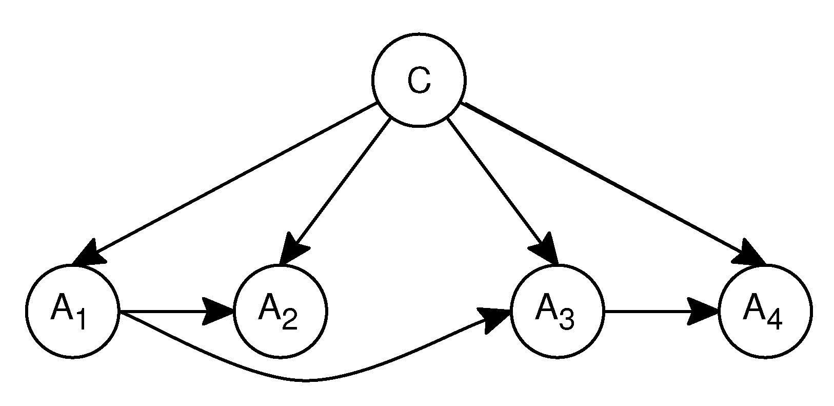Unfortunately, it has been proved that learning the optimal BN structure from an arbitrary BN search space of discrete variables is an non-deterministic polynomial-time hard (NP-hard) problem [1].One of the most effective BN classifiers, in the sense that its predictive performance is competitive with state-of-the-art classifiers [2], is the so-called naive Bayes (NB). NB is the simplest form of BN classifiers. It runs on labeled training instances and is driven by the conditional independence assumption that all attributes are fully independent of each other given the class. The NB classifier has the simple structure shown in Figure 1, where every attribute $A_i$ (every leaf in the network) is independent from the rest of the attributes, given the state of the class variable C (the root in the network). However, it is obvious that the conditional independence assumption in NB is often violated in real-world applications, which will affect its performance with complex attribute dependencies [3,4].

Figure 1. An example of naive Bayes (NB).

In order to effectively mitigate the assumption of independent attributes for the NB classifier, appropriate structures and approaches are needed to manipulate independence assertions [5,6,7]. Among the numerous Bayesian learning approaches, semi-naive Bayesian classifiers which utilize one-dependence estimators (ODEs) have been shown to be able to approximate the ground-truth attribute dependencies; meanwhile, the probability estimation in ODEs is effective, thus leading to excellent performance. Representative approaches include tree-augmented naive Bayesian (TAN) [8], hidden naive Bayes (HNB) [9], aggregating one-dependence estimators (AODE) [10], weighted average of one-dependence estimators (WAODE) [11].

To the best of our knowledge, few studies have focused on attribute value weighting in terms of Bayesian networks [12]. The attribute value weighting approach is a more fine-grained weighting approach, e.g., when dealing with the pregnancy-related disease classification problem and trying to analyze the importance of gender attributes. It is obvious that the value of the male gender attribute has no effect on the class value (pregnancy-related disease), whereas the value of the female gender attribute has a great effect on the class value. It will be interesting to study whether a better performance can be achieved by combining attribute value weighting with the ODEs. The resulting model which combines attribute value weighting with the ODEs inherits the effectiveness of ODEs; meanwhile, this approach is a new paradigm of weighting approach in classification learning.

In this study, we propose a new paradigm based on a simple, efficient, and effective attribute value weighting approach, called attribute value weighted average of one-dependence estimators (AVWAODE). Our AVWAODE approach is well balanced between the ground-truth dependencies approximation and the effectiveness of probability estimation. We extend the current classification learning utilizing ODEs into the next level by introducing a new set of weight space to the problem. It is a new approach to calculating the discriminative weights for ODEs using the filter approach. We assume that the significance of each ODE can be decomposed, and in the structure of highly predictive ODE, the different root attribute value should be strongly associated with the class. Based on these assumptions, we assign a different weight to each ODE by computing the correlation between the root attribute value and the class. In order to correctly measure the amount of correlation between the root attribute value and the class, our approach uses two different attribute value weighting measures: the Kullback–Leibler (KL) measure and the information gain (IG) measure, and thus two different versions are created, which are simply denoted by AVWAODE-KL and AVWAODE-IG, respectively. We conducted two groups of extensive empirical comparisons with many state-of-the-art Bayesian classifiers using 36 University of California at Irvine (UCI) datasets published on the main website of the WEKA platform [13,14]. Extensive experiments show that both AVWAODE-KL and AVWAODE-IG can achieve better performance than these state-of-the-art Bayesian classifiers used to compare.

The rest of the paper is organized as follows. In Section 2, we summarize the existing Bayesian networks learning utilizing ODEs. In Section 3, we propose our AVWAODE approach. In Section 4, we describe the experimental setup and results in detail. In Section 5, we draw our conclusions and outline the main directions for our future work.

2. Related Work

Learning Bayesian networks from data is a rapidly growing field of research that has seen a great deal of activity in recent years [15,16]. The notion of x-dependence estimators (x-DE) was proposed by Sahami [17]; x-DE allows each attribute to depend, at most, on only other x attributes in addition to the class. Webb et al. [18] defined the averaged n-dependence estimators (AnDE) family of algorithms. AnDE further relaxes the independence assumption. Extensive experimental evaluation shows that the bias-variance trade-off for averaged 2-dependence estimators (A2DE) results in strong predictive accuracy over a wide range of data sets [18]. A2DE proves to be a computationally tractable version of AnDE that delivers strong classification accuracy for large data without any parameter tuning.

To maintain efficiency, the Bayesian network appears desirable to restrict classifiers to ODEs [19]. A comparative study of linear combination schemes for superparent-one-dependence estimators was proposed by Yang [20]. Approaches which utilize ODEs have demonstrated remarkable performance [21,22]. Different from totally ignoring the attribute dependencies as naive Bayes or taking maximum flexibility for modelling dependencies as the Bayesian network, ODEs try to exploit attribute dependencies in moderate orders. By allowing one-order attribute dependencies, ODEs have been shown to be able to approximate the ground-truth attribute dependencies, whilst keeping the effectiveness of probability estimation, thus leading to excellent performance. In ODEs, directed arcs can be used to explicitly represent the joint probability distribution. The class variable is the parent of every attribute; meanwhile, every attribute has another attribute node as its parents; each attribute is independent of its nondescendants given the state of its parents. Using the independence statements encoded in ODEs, the joint probability distribution is uniquely determined by these local conditional distributions. These independencies are then used to reduce the number of parameters and to characterize the joint probability distribution.

ODEs restrict each attribute to depending only on one parent in addition to the class. If we assume that $A_1,A_2,\cdots ,A_m$ are m attributes, then a test instance x can be represented by an attribute value vector $<a_1,a_2,\cdots ,a_m>$, where $a_i$ denotes the value of the i-th attribute $A_i$; under the attribute independence assumption, Equation (1) is used to classify the test instance x:

$$c\left(x\right)=\arg \underset{c\in C}{\max }P\left(c\right)\prod _{i=1}^{m}P\left(a_i\right|a_{ip},c),$$

(1)

where $a_{ip}$ is the attribute value of $A_{ip}$, which is the attribute parent of $A_i$.

Friedman et al. [8] proposed tree-augmented naive Bayesian (TAN). The TAN algorithm builds a maximum weighted spanning tree; the conditional mutual information between each pair of attributes is computed, in which the vertices are the attributes; they finally transform the resulting undirected tree to a directed one by choosing a root variable and setting the direction of all edges to be outward from it. In TAN, the class variable has no parents and each attribute can only depend on another attribute parent in addition to the class; each attribute can have one augmenting edge pointing to it. The example of TAN is shown in Figure 2.

Figure 2. An example of tree-augmented naive Bayesian (TAN).

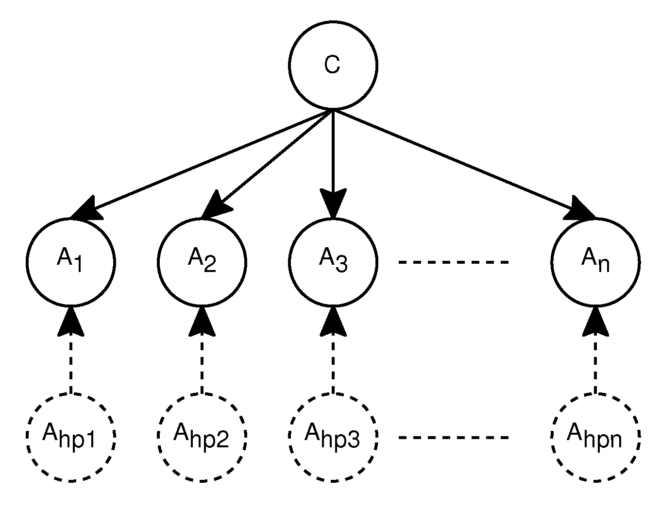
Jiang et al. [9] proposed a structure extension-based algorithm (HNB), which is based on ODEs; each attribute in HNB has a hidden parent that is a mixture of the weighted influences from all other attributes. HNB uses conditional mutual information to estimate the weights directly from data, and establishes a novel model that can consider the influences of all the attributes; it avoids learning with intractable computational complexity. The structure of HNB is shown in Figure 3.

Figure 3. A structure of hidden naive Bayes (HNB).

The approach of AODE [10] is to select a limited class of ODE and to aggregate the predictions of all qualified classifiers where there is a single attribute that is the parent of all other attributes. In order to avoid including models for which the base probability estimates are inaccurate, the AODE approach excludes models where the training data contain fewer than 30 examples of the value for $a_i$ of the parent attribute $A_i$. An example of the aggregate of AODE is shown in Figure 4.

Figure 4. An example of aggregating one-dependence estimators (AODE).

AODE classifies a test instance x using Equation (2).

$$c\left(x\right)=\arg \underset{c\in C}{\max }\left(\frac{{\sum }_{i=1\mathsf{\Lambda }F\left(a_i\right)\ge 30}^{m}P(a_i,c){\prod }_{k=1,k\ne i}^{m}P\left(a_k\right|a_i,c)}{numParent}\right),$$

(2)

where $F\left(a_i\right)$ is a count of the frequency of training instances having attribute value $a_i$, and is used to enforce the frequency limit; $numParent$ is the number of the root attributes, which satisfy the condition that the training instances contain more than 30 instances with the value $a_i$ for the parent attribute $A_i$.

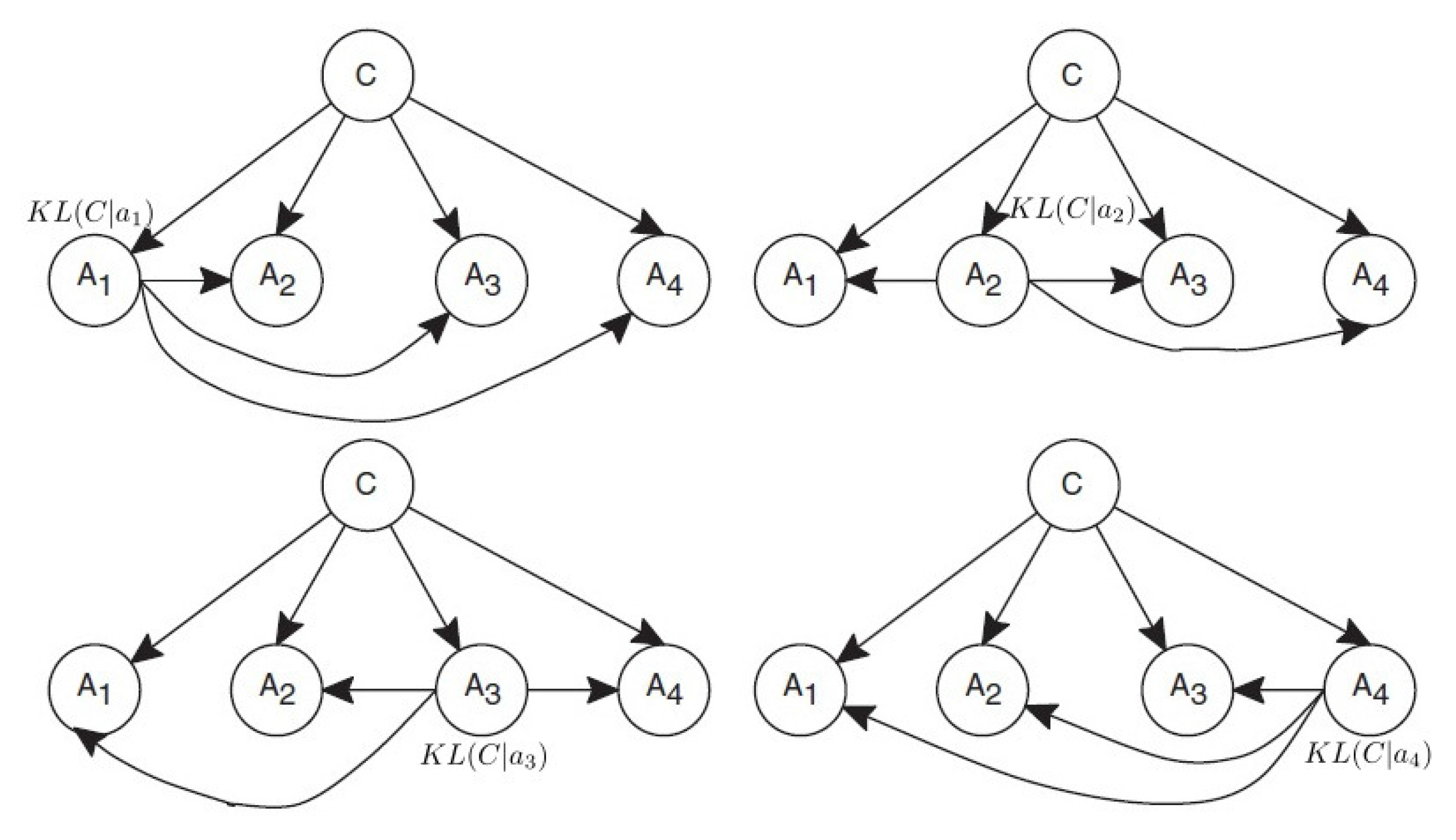
However, all ODEs in AODE have the same weights and are treated equally. WAODE [11] was proposed to assign different weights to different ODEs. In WAODE, a special ODE is built for each attribute. Namely, each attribute is set as the root attribute once and each special ODE is assigned a different weight. An example of the aggregate of WAODE is shown in Figure 5.

Figure 5. An example of weighted average of one-dependence estimators (WAODE).

WAODE classifies a test instance x using the following Equation (3).

$$c\left(x\right)=\arg \underset{c\in C}{\max }\left(\frac{{\sum }_{i=1}^m{W}_{i}P(a_i,c){\prod }_{k=1,k\ne i}^{m}P\left(a_k\right|a_i,c)}{{\sum }_{i=1}^m{W}_i}\right),$$

(3)

where $W_i$ is the weight of the ODE while the attribute $A_i$ is set as the root attribute, which is the parent of all other attributes. The WAODE approach assigns weight to each ODE according to the relationship between the root attribute and the class; it uses the mutual information $I_P(A_i;C)$ between the root attribute $A_i$ and the class variable C to define the weight $W_i$. The detailed Equation is:

$$W_i=I_P(A_i;C)=\sum _{a_i,c}P(a_i,c)\log \frac{P(a_i,c)}{P\left(a_i\right)P\left(c\right)}.$$

(4)

3. AVWAODE Approach

The remarkable performance of semi-naive Bayesian classifiers utilizing ODEs suggests that ODEs are well balanced between the attribute dependencies assumption and the effectiveness of probability estimation. To the best of our knowledge, few studies have focused on attribute value weighting in terms of Bayesian networks [12]. Each attribute takes on a number of discrete values, and each discrete value has different importance with respect to the target. Therefore, the attribute value weighting approach is a more fine-grained weighting approach. It is interesting to study whether a better performance can be achieved by exploiting the ODEs while using the attribute value weighting approach. The resulting model which combines attribute value weighting with the ODEs inherits the effectiveness of ODEs; meanwhile, this approach is a new paradigm of weighting approach in Bayesian classification learning.

In this study, we extend the current classification learning utilizing ODEs into the next level by introducing a new set of weight space to the problem. Therefore, this study proposes a new dimension of weighting approach by assigning weights according to attribute values. We propose a new paradigm based on a simple, efficient, and effective attribute value weighting approach, called attribute value weighted average of one-dependence estimators (AVWAODE). Our AVWAODE approach is well balanced between the ground-truth dependencies approximation and the effectiveness of probability estimation. It is a new method for calculating discriminative weights for ODEs using the filter approach. The basic assumption of our AVWAODE approach is that the root attribute value should be strongly associated with the class in the structure of highly predictive ODE, and in ODEs; when a certain root attribute value is observed, it gives a certain amount of information to the class. The more information a root attribute value provides to the class, the more important the root attribute value becomes.

In AVWAODE, a special ODE is built for each attribute. Namely, each attribute is set as the root attribute once and each special ODE is assigned a different weight. Different from the existing WAODE approach which assigns different weights to different ODEs according to the relationship between the root attribute and the class, our AVWAODE approach assigns discriminative weights to different ODEs by computing the correlation between the root attribute value and the class. Since the weight of each special ODE is associated with the root attribute value, AVWAODE uses Equation (5) to classify a test instance x.

$$c\left(x\right)=\arg \underset{c\in C}{\max }\left(\frac{{\sum }_{i=1}^m{W}_{i,a_i}P(a_i,c){\prod }_{k=1,k\ne i}^{m}P\left(a_k\right|a_i,c)}{{\sum }_{i=1}^m{W}_{i,a_i}}\right),$$

(5)

where $W_{i,a_i}$ is the weight of the ODE when the root attribute $A_i$ has the attribute value $a_i$. The base probabilities $P(a_i,c)$ and $P\left(a_k\right|a_i,c)$ are estimated using the m-estimate as follows:

$$P(a_i,c)=\frac{F(a_i,c)+1.0/(n_i\ast n_c)}{n+1.0},$$

(6)

$$P\left(a_k\right|a_i,c)=\frac{F(a_k,a_i,c)+1.0/n_k}{F(a_i,c)+1.0},$$

(7)

where $F(•)$ is the frequency with which a combination of terms appears in the training data, n is the number of training instances, $n_i$ is the number of values of the root attribute $A_i$, $n_k$ is the number of values of the leaf attribute $A_k$, and $n_c$ is the number of classes.

Now, the only question left to answer is how to use a proper measure which can correctly quantify the amount of correlation between the root attribute value and the class. To address this question, our approach uses two different attribute value weighting measures: the Kullback–Leibler (KL) measure and the information gain (IG) measure, and thus two different versions are created, which are simply denoted by AVWAODE-KL and AVWAODE-IG, respectively. Note that KL and IG are two widely used measures already presented in the existing literature; we just redefine them following our proposed methods.

3.1. AVWAODE-KL

The first candidate that can be used in our approach is the KL measure, which is a widely used method for calculating the correlation between the class variable and an attribute value [23]. The KL measure calculates the distances of different posterior probabilities from the prior probabilities. The main idea is that the KL measure becomes more reliable as the frequency of a specific attribute value increases. It originally was proposed in the article [24]. The KL measure calculates the average mutual information between the events c and the attribute value $a_i$ with the expectation taken with respect to a posteriori probability distribution of C [23]. The KL measure uses Equation (8) to quantify the information content of an attribute value $a_i$:

$$KL\left(C\right|a_i)=\sum _{c}P\left(c\right|a_i)\log \frac{P\left(c\right|a_i)}{P\left(c\right)},$$

(8)

where $KL\left(C\right|a_i)$ represents the attribute value-class correlation.

It is quite an intuitive argument that if the root attribute value $a_i$ gets a higher KL value, the ODE will deserve a higher weight. Therefore, we use the $KL\left(C\right|a_i)$ between the root attribute value $a_i$ and the class C to define the weight $W_{i,a_i}$ of the ODE as:

$$W_{i,a_i}=KL\left(C\right|a_i)=\sum _{c}P\left(c\right|a_i)\log \frac{P\left(c\right|a_i)}{P\left(c\right)},$$

(9)

where $a_i$ is the attribute value of the root attribute, which is the parent of all other attributes. An example of AVWAODE-KL is shown in Figure 6.

Figure 6. An example of attribute value weighted average of one-dependence estimators (AVWAODE)-KL.

The detailed learning algorithm for our AVWAODE approach using the KL measure (AVWAODE-KL) is described briefly as Algorithm 1.

Algorithm 1: AVWAODE-KL (D, x)
Input: A training dataset D and a test instance x  Output: Class label $c\left(x\right)$ of x
1.	For each class value c
2.	Compute $P\left(c\right)$ from D
3.	For each attribute value $a_i$
4.	Compute $F(a_i,c)$ from D
5.	Compute $P(a_i,c)$ by Equation (6)
6.	For each attribute value $a_k$ ($k\ne i$)
7.	Compute $F(a_k,a_i,c)$ from D
8.	Compute $P\left(a_k\right|a_i,c)$ by Equation (7)
9.	For each attribute value $a_i$
10.	Compute $F\left(a_i\right)$ from D
11.	Compute $W_{i,a_i}$ by Equation (9)
12.	Estimate the class label $c\left(x\right)$ for x using Equation (5)
13.	Return the class label $c\left(x\right)$ for x

Compared to the well-known AODE, AVWAODE-KL requires some additional training time to compute the weights of all the attribute values. According to the algorithm given above, the additional training time complexity for computing these weights is only $O\left(n_{c}mv\right)$; where $n_c$ is the number of classes, m is the number of attributes, and v is the average number of values for an attribute. Therefore, AVWAODE-KL has only a training time complexity of $O(n{m}^2+n_{c}mv)$, where n is the number of training instances. Note that $n_{c}v$ is generally much less than $nm$ in reality. If we only take the highest order term, the training time complexity is still $O\left(n{m}^2\right)$, which is the same as AODE. In addition, the classification time complexity of AVWAODE-KL is $O\left(n_c{m}^2\right)$, which is also the same as AODE. All of this means that AVWAODE-KL is simple and efficient.

3.2. AVWAODE-IG

The second candidate that can be used in our approach is the IG measure, which is a widely used method for calculating the importance of attributes [5,25]. The C4.5 approach [2] uses the IG measure to construct the decision tree for classifying objects. The information gain used in the C4.5 approach [2] is defined as:

$$H\left(C\right)-H\left(C\right|A_i)=\sum _{a_i}P\left(a_i\right)\sum _{c}P\left(c\right|a_i)logP\left(c\right|a_i)-\sum _{c}P\left(c\right)logP\left(c\right).$$

(10)

Equation (10) computes the difference between the entropy of a priori distribution and the entropy of a posteriori distribution of the class, and the C4.5 approach uses the difference value as the metric for deciding the branching node. The value of the IG measure can represent the significance of the attribute; the bigger the value is, the greater impact of the attribute when classifying the test instance. The correlation between the attribute $A_i$ and the class C can be measured by Equation (10). Since we require discriminative power for an attribute value, we cannot use Equation (10) directly as the measure of the discriminative power for an attribute value. The IG measure calculates the correlation between an attribute value $a_i$ and the class variable C by:

$$IG\left(C\right|a_i)=\sum _{c}P\left(c\right|a_i)logP\left(c\right|a_i)-\sum _{c}P\left(c\right)logP\left(c\right).$$

(11)

It is quite an intuitive argument that if the root attribute value $a_i$ gets a higher IG value, the ODE will deserve a higher weight. Therefore, we use the $IG\left(C\right|a_i)$ between the root attribute value $a_i$ and the class C to define the weight $W_{i,a_i}$ of the ODE as:

$$W_{i,a_i}=IG\left(C\right|a_i)=\sum _{c}P\left(c\right|a_i)logP\left(c\right|a_i)-\sum _{c}P\left(c\right)logP\left(c\right),$$

(12)

where $a_i$ is the attribute value of the root attribute, which is the parent of all other attributes. An example of AVWAODE-IG is shown in Figure 7.

Figure 7. An example of AVWAODE-IG.

The training time complexity and the classification time complexity of AVWAODE-IG is the same as AVWAODE-KL. In order to save space, we do not repeat the detailed analysis here.

4. Experiments and Results

In order to validate the classification performance of AVWAODE, we ran our experiments on all the 36 UCI datasets [26] published on the main web site of Weka platform [13,14]. In our experiments, missing values are replaced with the modes and means of the corresponding attribute values from the available data. Numeric attribute values are discretized using the unsupervised ten-bin discretization implemented in Weka platform. Additionally, we manually delete three useless attributes: the attribute “Hospital Number” in the dataset “colic.ORIG”, the attribute “instance name" in the dataset “splice”, and the attribute “animal” in the dataset “zoo”.

We compare the performance of AVWAODE with some state-of-the-art Bayesian classifiers: TAN [8], HNB [9], AODE [10], WAODE [11], NB [2] and A2DE [18]. We conduct extensive empirical comparisons in two groups with these state-of-the-art models in terms of the classification accuracy. In the first group, we compared AVWAODE-KL with all of these models, and in the second group, we compared AVWAODE-IG with these competitors.

Table 1 and Table 2 show the detailed results of the comparisons in terms of the classification accuracy. All of the classification accuracy estimates were obtained by averaging the results from 10 separate runs in a stratified ten-fold cross-validation. We then conducted corrected paired two-tailed t-tests at the 95% significance level [27] in order to compare our AVWAODE-KL and AVWAODE-IG with each of their competitors: TAN, HNB, AODE, WAODE, NB, and A2DE. The averages and the $Win$/$Tie$/$Lose$ (W/T/L) values are summarized at the bottom of the tables. Each entry’s W/T/L in the tables implies that, compared to their competitors, AVWAODE-KL and AVWAODE-IG win on W datasets, tie on T datasets, and lose on L datasets. The average (arithmetic mean) of each algorithm across all datasets provides a gross indicator of the relative performance in addition to the other statistics.

Table 1. Accuracy comparisons for AVWAODE-KL versus TAN, HNB, AODE, WAODE, NB, and A2DE.

Dataset	AVWAODE-KL	TAN	HNB	AODE	WAODE	NB	A2DE
anneal	98.86	96.73 •	97.74 •	96.74 •	98.56	94.32 •	98.36
anneal.ORIG	91.10	90.49	89.87	88.79 •	89.80 •	88.16 •	90.32
audiology	76.17	65.35 •	69.04 •	71.66 •	76.26	71.40 •	74.84
autos	80.75	72.54 •	75.49	73.48 •	80.36	63.97 •	76.97
balance-scale	88.53	86.14 •	89.14	89.78	89.28	91.44 ∘	91.44 ∘
breast-cancer	70.67	69.53	73.09	72.53	71.97	72.94	70.63
breast-w	96.08	95.45	95.67	97.11	96.57	97.30	97.17
colic	80.96	80.11	81.44	80.90	80.66	78.86	81.12
colic.ORIG	75.50	67.71 •	75.66	75.30	75.93	74.21	76.68
credit-a	85.17	84.10	85.80	85.91	84.43	84.74	84.83
credit-g	75.31	74.88	76.29	76.42	76.38	75.93	75.19
diabetes	75.03	76.31	76.00	76.37	75.83	75.68	75.74
glass	59.47	58.69	59.02	61.13	59.62	57.69	63.14
heart-c	81.98	79.70	82.31	82.48	82.61	83.44	81.75
heart-h	82.29	81.27	83.21	84.06	83.11	83.64	81.74
heart-statlog	82.85	79.48	82.70	83.67	82.30	83.78	83.81
hepatitis	83.82	83.00	83.92	84.82	84.14	84.06	85.26
hypothyroid	93.42	93.36	93.49	93.53	93.54	92.79 •	93.17
ionosphere	92.11	91.34	92.00	92.08	92.94	90.86	92.88
iris	95.13	94.27	93.93	94.47	95.73	94.33	94.33
kr-vs-kp	94.32	92.88 •	92.36 •	91.01 •	94.18	87.79 •	93.69
labor	90.90	89.00	92.73	95.30	91.73	96.70	92.67
letter	89.24	82.69 •	84.68 •	85.54 •	88.86 •	70.09 •	80.44 •
lymph	85.35	83.69	83.90	86.25	84.16	85.97	84.75
mushroom	99.99	99.99	99.94	99.95	99.98	95.52 •	99.52 •
primary-tumor	48.14	44.77	47.66	47.67	47.94	47.20	47.32
segment	95.41	93.91 •	93.72 •	92.94 •	95.06	89.03 •	94.83
sick	98.11	97.70 •	97.77	97.51 •	97.99	96.78 •	97.55 •
sonar	77.46	75.34	81.75	79.04	78.28	76.35	74.30
soybean	94.28	94.98	93.88	93.28	94.33	92.20 •	94.45
splice	96.31	94.95 •	95.84 •	96.12 •	96.36 •	95.42 •	95.40 •
vehicle	73.35	73.35	72.15	71.62	73.09	61.03 •	72.48
vote	94.46	94.43	94.43	94.52	94.46	90.21 •	93.26
vowel	92.67	91.89	91.34	89.52 •	92.56	66.09 •	92.62
waveform-5000	83.61	80.44 •	83.79	84.24	84.00	79.97 •	82.17
zoo	98.50	96.63	97.73	94.66	98.11	94.37	95.65
Average	85.48	83.53	84.99	85.01	85.59	82.34	85.01
W/T/L	-	11/25/0	6/30/0	9/27/0	2/34/0	16/19/1	5/30/1

∘, • statistically significant improvement or degradation over AVWAODE-KL.

Table 2. Accuracy comparisons for AVWAODE-IG versus TAN, HNB, AODE, WAODE, NB, and A2DE.

Dataset	AVWAODE-IG	TAN	HNB	AODE	WAODE	NB	A2DE
anneal	98.75	96.73 •	97.74 •	96.74 •	98.56	94.32 •	98.36
anneal.ORIG	89.45	90.49	89.87	88.79	89.80	88.16	90.32
audiology	76.04	65.35 •	69.04 •	71.66 •	76.26 •	71.40 •	74.84
autos	80.16	72.54 •	75.49	73.48 •	80.36	63.97 •	76.97
balance-scale	88.46	86.14 •	89.14	89.78	89.28	91.44 ∘	91.44 ∘
breast-cancer	71.84	69.53	73.09	72.53	71.97	72.94	70.63
breast-w	96.25	95.45	95.67	97.11	96.57	97.30	97.17
colic	80.93	80.11	81.44	80.90	80.66	78.86	81.12
colic.ORIG	75.33	67.71 •	75.66	75.30	75.93	74.21	76.68
credit-a	85.45	84.10	85.80	85.91	84.43	84.74	84.83
credit-g	75.79	74.88	76.29	76.42	76.38	75.93	75.19
diabetes	75.60	76.31	76.00	76.37	75.83	75.68	75.74
glass	58.95	58.69	59.02	61.13	59.62	57.69	63.14
heart-c	82.15	79.70	82.31	82.48	82.61	83.44	81.75
heart-h	81.98	81.27	83.21	84.06	83.11	83.64	81.74
heart-statlog	82.52	79.48	82.70	83.67	82.30	83.78	83.81
hepatitis	84.52	83.00	83.92	84.82	84.14	84.06	85.26
hypothyroid	93.48	93.36	93.49	93.53	93.54	92.79 •	93.17
ionosphere	93.02	91.34	92.00	92.08	92.94	90.86 •	92.88
iris	95.13	94.27	93.93	94.47	95.73	94.33	94.33
kr-vs-kp	94.13	92.88 •	92.36 •	91.01 •	94.18	87.79 •	93.69
labor	91.40	89.00	92.73	95.30	91.73	96.70	92.67
letter	89.24	82.69 •	84.68 •	85.54 •	88.86 •	70.09 •	80.44 •
lymph	84.47	83.69	83.90	86.25	84.16	85.97	84.75
mushroom	99.99	99.99	99.94	99.95	99.98	95.52 •	99.52 •
primary-tumor	48.50	44.77	47.66	47.67	47.94	47.20	47.32
segment	95.41	93.91 •	93.72 •	92.94 •	95.06	89.03 •	94.83
sick	98.03	97.70 •	97.77	97.51 •	97.99	96.78 •	97.55 •
sonar	77.18	75.34	81.75	79.04	78.28	76.35	74.30
soybean	94.50	94.98	93.88	93.28 •	94.33	92.20 •	94.45
splice	96.39	94.95 •	95.84 •	96.12	96.36	95.42 •	95.40 •
vehicle	73.34	73.35	72.15	71.62	73.09	61.03 •	72.48
vote	94.25	94.43	94.43	94.52	94.46	90.21 •	93.26
vowel	92.67	91.89	91.34	89.52 •	92.56	66.09 •	92.62
waveform-5000	83.61	80.44 •	83.79	84.24	84.00	79.97 •	82.17 •
zoo	98.41	96.63	97.73	94.66	98.11	94.37	95.65
Average	85.48	83.53	84.99	85.01	85.59	82.34	85.01
W/T/L	-	11/25/0	6/30/0	9/27/0	1/35/0	16/19/1	5/30/1

∘, • statistically significant improvement or degradation over AVWAODE-IG.

Then, we employ a corrected paired two-tailed t-test with the $p=0.05$ significance level [27] to compare each pair of algorithms. Table 3 and Table 4 show the summary test results with regard to AVWAODE-KL and AVWAODE-IG, respectively. In these tables, for each entry $i\left(j\right)$, i is the number of datasets on which the algorithm in the column achieves higher classification accuracy than the algorithm in the corresponding row, and j is the number of datasets on which the algorithm in the column achieves significant wins with the $p=0.05$ significance level [27] with regard to the algorithm in the corresponding row.

Table 3. Summary test results with regard to AVWAODE-KL.

Algorithm	AVWAODE-KL	TAN	HNB	AODE	WAODE	NB	A2DE
AVWAODE-KL	-	3 (0)	14 (0)	17 (0)	20 (0)	11 (1)	11 (1)
TAN	33 (11)	-	27 (6)	27 (9)	31 (10)	17 (6)	25 (9)
HNB	22 (6)	9 (0)	-	22 (2)	27 (5)	10 (2)	18 (5)
AODE	19 (9)	9 (3)	14 (3)	-	20 (9)	6 (1)	19 (5)
WAODE	16 (2)	5 (0)	9 (0)	16 (0)	-	9 (1)	13 (1)
NB	25 (16)	19 (13)	26 (16)	30 (13)	27 (17)	-	26 (13)
A2DE	25 (5)	11 (2)	18 (4)	17 (3)	23 (5)	9 (0)	-

Table 4. Summary test results with regard to AVWAODE-IG.

Algorithm	AVWAODE-IG	TAN	HNB	AODE	WAODE	NB	A2DE
AVWAODE-IG	-	6 (0)	17 (0)	17 (0)	19 (0)	10 (1)	11 (1)
TAN	30 (11)	-	27 (6)	27 (9)	31 (10)	17 (6)	25 (9)
HNB	19 (6)	9 (0)	-	22 (2)	27 (5)	10 (2)	18 (5)
AODE	19 (9)	9 (3)	14 (3)	-	20 (9)	6 (1)	19 (5)
WAODE	17 (1)	5 (0)	9 (0)	16 (0)	-	9 (1)	13 (1)
NB	26 (16)	19 (13)	26 (16)	30 (13)	27 (17)	-	26 (13)
A2DE	25 (5)	11 (2)	18 (4)	17 (3)	23 (5)	9 (0)	-

Table 5 and Table 6 show the ranking test results with regard to AVWAODE-KL and AVWAODE-IG, respectively. In these tables, the first column is the difference between the total number of wins and the total number of losses that the corresponding algorithm achieves compared with all the other algorithms, which is used to generate the ranking. The second and third columns represent the total numbers of wins and losses, respectively.

Table 5. Ranking test results with regard to AVWAODE-KL.

Resultset	Wins−Losses	Wins	Losses
AVWAODE-KL	47	49	2
WAODE	42	46	4
A2DE	15	34	19
HNB	9	29	20
AODE	−3	27	30
TAN	−33	18	51
NB	−77	11	88

Table 6. Ranking test results with regard to AVWAODE-IG.

Resultset	Wins−Losses	Wins	Losses
AVWAODE-IG	46	48	2
WAODE	43	46	3
A2DE	15	34	19
HNB	9	29	20
AODE	−3	27	30
TAN	−33	18	51
NB	−77	11	88

According to these comparisons, we can see that both AVWAODE-KL and AVWAODE-IG perform better than TAN, HNB, AODE, WAODE, NB, and A2DE. We summarize the main features of these comparisons as follows.

• Both AVWAODE-KL and AVWAODE-IG significantly outperform NB with 16 wins and one loss, and they also outperform TAN with 11 wins and zero losses.
• Both AVWAODE-KL and AVWAODE-IG perform notably better than HNB on six datasets and worse on zero datasets, and also better than A2DE on five datasets and worse on one dataset.
• Both AVWAODE-KL and AVWAODE-IG are markedly better than AODE with nine wins and zero losses.
• Both AVWAODE-KL and AVWAODE-IG perform substantially better than WAODE on two datasets and one datset, respectively.
• Seen from the ranking test results, our proposed algorithms are always the best ones, and NB is the worst one. The overall ranking (descending order) is AVWAODE-KL (AVWAODE-IG), WAODE, A2DE, HNB, AODE, TAN and NB, respectively.
• The results of these comparisons suggest that assigning discriminative weights to different ODEs by computing the correlation between the root attribute value and the class is highly effective when setting weights for ODEs.

Yet at the same time, based on the accuracy results presented in Table 1 and Table 2, we take advantage of KEEL Data-Mining Software Tool [28,29] to complete the Wilcoxon signed-ranks test [30,31] to thoroughly compare each pair of algorithms. The Wilcoxon signed-ranks test is a non-parametric statistical test, which ranks the differences in performances of two algorithms for each dataset, ignoring the signs, and compares the ranks for positive and negative differences. Table 7, Table 8, Table 9 and Table 10 summarize the detailed results of the nonparametric statistical comparisons based on the Wilcoxon test. According to the table, for the exact critical values in the Wilcoxon test at a confidence level of $\alpha =0.05$ ($\alpha =0.1$) and with datasets where $N=36$, two algorithms are considered “significantly different" if the smaller of $R^{+}$ and $R^{-}$ is equal to or less than 208 (227), and thus we could reject the null hypothesis. ∘ indicates that the algorithm in the column improves the algorithm in the corresponding row, and • indicates that the algorithm in the row improves the algorithm in the corresponding column. According to these comparisons, we can see that both AVWAODE-KL and AVWAODE-IG performed significantly better than NB, and TAN, and AVWAODE-IG performed even significantly better than A2DE at a confidence level of $\alpha =0.1$.

Table 7. Ranks computed by the Wilcoxon test on AVWAODE-KL.

Algorithm	AVWAODE-KL	TAN	HNB	AODE	WAODE	NB	A2DE
AVWAODE-KL	-	636.5	426.5	370.5	264.5	525.0	427.0
TAN	29.5	-	100.0	130.0	35.0	362.5	131.5
HNB	239.5	566.0	-	312.5	172.0	521.0	298.0
AODE	295.5	536.0	353.5	-	259.5	593.0	315.5
WAODE	401.5	631.0	494.0	406.5	-	547.0	446.0
NB	141.0	303.5	145.0	73.0	119.0	-	135.5
A2DE	239.0	534.5	368.0	350.5	220.0	530.5	-

Table 8. Summary of the Wilcoxon test on AVWAODE-KL. ∘: The algorithm in the column improves the algorithm in the corresponding row. •: The algorithm in the row improves the algorithm in the corresponding column. Lower diagonal level of significance $\alpha =0.05$; upper diagonal level of significance $\alpha =0.1$.

Algorithm	AVWAODE-KL	TAN	HNB	AODE	WAODE	NB	A2DE
AVWAODE-KL	-	•				•
TAN	∘	-	∘	∘	∘		∘
HNB		•	-		∘	•
AODE		•		-		•
WAODE		•	•		-	•	•
NB	∘		∘	∘	∘	-	∘
A2DE		•				•	-

Table 9. Ranks computed by the Wilcoxon test on AVWAODE-IG.

Algorithm	AVWAODE-IG	TAN	HNB	AODE	WAODE	NB	A2DE
AVWAODE-IG	-	628.0	431.5	380.5	255.0	525.5	440.5
TAN	38.0	-	100.0	130.0	35.0	362.5	131.5
HNB	234.5	566.0	-	312.5	172.0	521.0	298.0
AODE	285.5	536.0	353.5	-	259.5	593.0	315.5
WAODE	411.0	631.0	494.0	406.5	-	547.0	446.0
NB	140.5	303.5	145.0	73.0	119.0	-	135.5
A2DE	225.5	534.5	368.0	350.5	220.0	530.5	-

Table 10. Summary of the Wilcoxon test on AVWAODE-IG. ∘: The algorithm in the column improves the algorithm in the corresponding row. •: The algorithm in the row improves the algorithm in the corresponding column. Lower diagonal level of significance $\alpha =0.05$; upper diagonal level of significance $\alpha =0.1$.

Algorithm	AVWAODE-IG	TAN	HNB	AODE	WAODE	NB	A2DE
AVWAODE-IG	-	•				•	•
TAN	∘	-	∘	∘	∘		∘
HNB		•	-		∘	•
AODE		•		-		•
WAODE		•	•		-	•	•
NB	∘		∘	∘	∘	-	∘
A2DE		•				•	-

Additionally, in our experiments, we have also observed the performance of our proposed AVWAODE in terms of the area under the Receiver Operating Characteristics (ROC) curve (AUC) [25,32,33,34]. Table 11 and Table 12 show the detailed comparison results in terms of AUC. From these comparison results, we can find that our proposed AVWAODE is also very promising in terms of the area under the ROC curve. Please note that, in order to save space, we do not present the detailed summary test results, the ranking test results, and the Wilcoxon test results.

Table 11. Area under the ROC curve (AUC) comparisons for AVWAODE-KL versus TAN, HNB, AODE, WAODE, NB, and A2DE.

Dataset	AVWAODE-KL	TAN	HNB	AODE	WAODE	NB	A2DE
anneal	99.76	99.63	99.68	99.34 •	99.73	98.88 •	99.73
anneal.ORIG	97.24	96.80	96.78 •	95.71 •	97.01 •	95.45 •	96.91
audiology	97.73	95.92 •	96.39 •	96.98 •	97.67	96.93 •	97.66
autos	94.14	92.65	93.32	92.56	94.16	88.10 •	93.89
balance-scale	92.10	94.00 ∘	96.40 ∘	94.85 ∘	92.16	96.22 ∘	96.15 ∘
breast-cancer	68.13	65.36	68.78	70.81	68.53	70.18	66.75
breast-w	99.17	98.89	99.24	99.35	99.19	99.25	99.39
colic	86.30	85.58	86.88	86.60	86.54	84.36	84.55
colic.ORIG	83.04	72.02 •	82.65	82.29	84.35	81.18	83.11
credit-a	91.19	90.49	92.00	92.38	91.49	91.86	91.98
credit-g	77.56	77.10	80.32 ∘	79.69 ∘	78.81 ∘	79.10	77.56
diabetes	82.17	81.87	82.91	82.85	82.76	82.61	82.21
glass	83.90	80.73 •	81.76	82.64	83.75	80.17 •	82.27
heart-c	89.69	87.90	90.40	91.00 ∘	89.93	91.08	90.20
heart-h	88.11	87.09	89.34	89.97	88.66	90.04	88.47
heart-statlog	89.98	89.36	90.84	91.26	90.01	91.34	91.16
hepatitis	87.83	87.15	87.46	89.31	87.60	89.36	90.31
hypothyroid	84.76	83.16 •	83.47 •	84.03	84.64	83.45	84.01
ionosphere	97.96	98.05	97.43	97.32	98.20	93.69 •	98.19
iris	99.13	98.96	98.59	98.77	99.17	98.97	98.96
kr-vs-kp	98.49	98.26	98.21	97.42 •	98.57	95.19 •	98.27
labor	97.29	93.75	97.83	98.79	97.75	98.67	97.38
letter	99.68	99.15 •	99.40 •	99.45 •	99.66 •	97.12 •	98.98 •
lymph	92.18	91.98	93.43	93.16	92.41	92.88	92.67
mushroom	100.00	100.00	100.00	100.00	100.00	99.80 •	100.00 •
primary-tumor	83.57	80.97 •	82.65 •	82.89	83.64	82.79	82.94
segment	99.70	99.53 •	99.55 •	99.42 •	99.68 •	98.36 •	99.60 •
sick	98.68	98.08	97.53 •	97.07 •	98.82	95.87 •	98.28
sonar	88.35	83.79 •	90.33	88.92	89.17	85.50	83.59 •
soybean	99.70	99.79	99.76	99.57 •	99.69	99.48 •	99.70
splice	99.51	99.18 •	99.46 •	99.45	99.51	99.35 •	99.24 •
vehicle	91.05	91.77	91.02	90.76	90.96	83.47 •	91.21
vote	98.83	98.75	98.78	98.67	98.75	97.15 •	98.43
vowel	99.63	99.54	99.56	99.43 •	99.61	95.76 •	99.59
waveform-5000	96.19	94.50 •	96.52 ∘	96.60 ∘	96.38 ∘	95.32 •	95.35 •
zoo	99.96	99.91	99.96	99.92	99.96	99.92	99.88
Average	92.57	91.43	92.74	92.76	92.75	91.63	92.46
W/T/L	-	10/25/1	8/25/3	9/23/4	3/31/2	17/18/1	6/29/1

∘, • statistically significant improvement or degradation over AVWAODE-KL.

Table 12. AUC comparisons for AVWAODE-IG versus TAN, HNB, AODE, WAODE, NB, and A2DE.

Dataset	AVWAODE-IG	TAN	HNB	AODE	WAODE	NB	A2DE
anneal	99.76	99.63	99.68	99.34 •	99.73	98.88 •	99.73
anneal.ORIG	97.00	96.80	96.78	95.71 •	97.01	95.45 •	96.91
audiology	97.71	95.92 •	96.39 •	96.98 •	97.67	96.93 •	97.66
autos	94.14	92.65	93.32	92.56	94.16	88.10 •	93.89
balance-scale	92.10	94.00 ∘	96.40 ∘	94.85 ∘	92.16	96.22 ∘	96.15 ∘
breast-cancer	69.58	65.36	68.78	70.81	68.53	70.18	66.75
breast-w	99.21	98.89	99.24	99.35	99.19	99.25	99.39
colic	86.39	85.58	86.88	86.60	86.54	84.36	84.55
colic.ORIG	84.02	72.02 •	82.65	82.29	84.35	81.18	83.11
credit-a	91.18	90.49	92.00	92.38	91.49	91.86	91.98
credit-g	78.18	77.10	80.32 ∘	79.69 ∘	78.81	79.10	77.56
diabetes	82.66	81.87	82.91	82.85	82.76	82.61	82.21
glass	83.29	80.73	81.76	82.64	83.75	80.17 •	82.27
heart-c	89.51	87.90	90.40	91.00 ∘	89.93	91.08 ∘	90.20
heart-h	87.99	87.09	89.34	89.97	88.66	90.04	88.47
heart-statlog	89.58	89.36	90.84	91.26	90.01	91.34	91.16
hepatitis	87.90	87.15	87.46	89.31	87.60	89.36	90.31
hypothyroid	85.08	83.16 •	83.47 •	84.03	84.64	83.45 •	84.01
ionosphere	98.09	98.05	97.43	97.32	98.20	93.69 •	98.19
iris	99.13	98.96	98.59	98.77	99.17	98.97	98.96
kr-vs-kp	98.38	98.26	98.21	97.42 •	98.57 ∘	95.19 •	98.27
labor	97.17	93.75	97.83	98.79	97.75	98.67	97.38
letter	99.68	99.15 •	99.40 •	99.45 •	99.66 •	97.12 •	98.98 •
lymph	92.24	91.98	93.43	93.16	92.41	92.88	92.67
mushroom	100.00	100.00	100.00	100.00	100.00	99.80 •	100.00 •
primary-tumor	83.64	80.97 •	82.65 •	82.89	83.64	82.79	82.94
segment	99.70	99.53 •	99.55 •	99.42 •	99.68 •	98.36 •	99.60 •
sick	98.67	98.08 •	97.53 •	97.07 •	98.82	95.87 •	98.28
sonar	88.26	83.79 •	90.33	88.92	89.17	85.50	83.59 •
soybean	99.69	99.79	99.76	99.57 •	99.69	99.48 •	99.70
splice	99.52	99.18 •	99.46 •	99.45	99.51	99.35 •	99.24 •
vehicle	91.05	91.77	91.02	90.76	90.96	83.47 •	91.21
vote	98.90	98.75	98.78	98.67	98.75	97.15 •	98.43
vowel	99.63	99.54	99.56	99.43 •	99.61	95.76 •	99.59
waveform-5000	96.19	94.50 •	96.52 ∘	96.60 ∘	96.38 ∘	95.32 •	95.35 •
zoo	99.97	99.91	99.96	99.92	99.96	99.92	99.88
Average	92.64	91.43	92.74	92.76	92.75	91.63	92.46
W/T/L	-	10/25/1	7/26/3	9/23/4	2/32/2	18/16/2	6/29/1

∘, • statistically significant improvement or degradation over AVWAODE-IG.

5. Conclusions and Future Work

Of numerous proposals to improve the accuracy of naive Bayes by weakening its attribute independence assumption, semi-naive Bayesian classifiers which utilize one-dependence estimators (ODEs) have been shown to be able to approximate the ground-truth attribute dependencies; meanwhile, the probability estimation in ODEs is effective. In this study, we propose a new paradigm based on a simple, efficient, and effective attribute value weighting approach, called attribute value weighted average of one-dependence estimators (AVWAODE). Our AVWAODE approach is well balanced between the ground-truth dependencies approximation and the effectiveness of probability estimation. We assign discriminative weights to different ODEs by computing the correlation between the root attribute value and the class. Two different attribute value weighting measures, which are called the Kullback–Leibler (KL) measure and the information gain (IG) measure, are used to quantify the correlation between the root attribute value and the class, and thus two different versions are created, which are simply denoted by AVWAODE-KL and AVWAODE-IG, respectively. Extensive experiments show that both AVWAODE-KL and AVWAODE-IG achieve better performance than some other state-of-the-art ODE models used for comparison.

How to learn the weights is a crucial problem in our proposed AVWAODE approach. An interesting future work will be the exploration of more effective methods to estimate weights to improve our current AVWAODE versions. Furthermore, applying the proposed attribute value weighting approach to improve some other state-of-the-art classification models is another topic for our future work.