Article

On Macrostates in Complex Multi-Scale Systems

by
Harald Atmanspacher
Collegium Helveticum, University Zurich and ETH Zurich, 8092 Zurich, Switzerland
Entropy 2016, 18(12), 426; https://doi.org/10.3390/e18120426
Submission received: 20 October 2016 / Revised: 18 November 2016 / Accepted: 21 November 2016 / Published: 29 November 2016
(This article belongs to the Special Issue Information and Self-Organization)

Abstract

:
A characteristic feature of complex systems is their deep structure, meaning that the definition of their states and observables depends on the level, or the scale, at which the system is considered. This scale dependence is reflected in the distinction of micro- and macro-states, referring to lower and higher levels of description. There are several conceptual and formal frameworks to address the relation between them. Here, we focus on an approach in which macrostates are contextually emergent from (rather than fully reducible to) microstates and can be constructed by contextual partitions of the space of microstates. We discuss criteria for the stability of such partitions, in particular under the microstate dynamics, and outline some examples. Finally, we address the question of how macrostates arising from stable partitions can be identified as relevant or meaningful.

1. Introduction

1.1. Complex Systems

The concepts of complexity and the study of complex systems represent some of the most important challenges for research in contemporary science. Although one might say that its formal core lies in mathematics and physics, complexity in a broad sense is certainly one of the most interdisciplinary issues scientists of many backgrounds have to face today. Beyond the traditional disciplines of the natural sciences, the concept of complexity has even crossed the border to areas like psychology, sociology, economics and others. It is impossible to address all approaches and applications that are presently known comprehensively here; overviews from different eras and areas of complexity studies are due to Cowan et al. [1], Cohen and Stewart [2], Auyang [3], Scott [4], Shalizi [5], Gershenson et al. [6], Nicolis and Nicolis [7], Mitchell [8] and Hooker [9].
The study of complex systems includes a whole series of other interdisciplinary approaches: system theory (Bertalanffy [10]), cybernetics (Wiener [11]), self-organization (Foerster [12]), fractals (Mandelbrot [13]), synergetics (Haken [14]), dissipative (Nicolis and Prigogine [15]) and autopoietic systems (Maturana and Varela [16]), automata theory (Hopcroft and Ullmann [17], Wolfram [18]), network theory (Albert and Barabási [19], Boccaletti et al. [20], Newman et al. [21]), information geometry (Ali et al. [22], Cafaro and Mancini [23]), and more. In all of these approaches, the concept of information plays a significant role in one or another way, first due to Shannon and Weaver [24] and later also in other contexts (for overviews, see Zurek [25], Atmanspacher and Scheingraber [26], Kornwachs and Jacoby [27], Marijuàn and Conrad [28], Boffetta et al. [29], Crutchfield and Machta [30]).
An important predecessor of complexity theory is the theory of nonlinear dynamical systems, which originated from the early work of Poincaré and was further developed by Lyapunov, Hopf, Krylov, Kolmogorov, Smale and Ruelle, to mention just a few outstanding names. Prominent areas in the study of complex systems as far as it has evolved from nonlinear dynamics are deterministic chaos (Stewart [31], Lasota and Mackey [32]), coupled map lattices (Kaneko [33], Kaneko and Tsuda [34]), symbolic dynamics (Lind and Marcus [35]), self-organized criticality (Bak [36]) and computational mechanics (Shalizi and Crutchfield [37]).
This ample (and incomplete) list notwithstanding, it is fair to say that one important open question is the question for a fundamental theory with a universal range of applicability, e.g., in the sense of an axiomatic basis, of nonlinear dynamical systems. Although much progress has been achieved in understanding a large corpus of phenomenological features of dynamical systems, we do not have any compact set of basic equations (like Newton’s, Maxwell’s or Schrödinger’s equations) or postulates (like those of relativity theory) for a comprehensive, full-fledged, formal theory of nonlinear dynamical systems, and this applies to the concept of complexity, as well.
Which criteria does a system have to satisfy in order to be complex? This question is not yet answered comprehensively, either, but quite a few essential issues can be indicated. From a physical point of view, complex behavior typically (but not always) arises in situations far from thermal equilibrium. This is to say that one usually does not speak of a complex system if its behavior can be described by the laws of linear thermodynamics. The thermodynamic branch of a system typically becomes unstable before complex behavior emerges. In this manner the concepts of stability and instability become indispensable elements of any proper understanding of complex systems. Recent work by Cafaro et al. [38] emphasizes other intriguing links between complexity, information and thermodynamics.
In addition, complex systems usually are open systems, exchanging energy and/or matter (and/or information) with their environment. Other essential features are internal self-reference, leading to self-organized cooperative behavior, and external constraints, such as control parameters. Moreover, complex systems are often multi-scale systems, meaning that the definition of their states and observables differs on different spatial and temporal scales (which are often used to define different levels of description). Corresponding microstates and macrostates and their associated observables are in general non-trivially related to one another.

1.2. Defining Complexity

Subsequent to algorithmic complexity measures (Solomonoff [39], Kolmogorov [40], Chaitin [41], Martin-Löf [42]), a remarkable number of different definitions of complexity have been suggested over the decades. Classic overviews are due to Lindgren and Nordahl [43], Grassberger [44,45], Wackerbauer et al. [46] or Lloyd [47]. Though some complexity measures are more popular than others, there are no rigorous criteria to select a “correct” definition and reject the rest.
It appears that for a proper characterization of complexity, one of the fundaments of scientific methodology, the search for universality, must be complemented by an unavoidable context dependence or contextuality. An important example for such contexts is the role of the environment, including measuring instruments (see Remark A1). Another case in point is the model class an observer has in mind when modeling a complex system (Crutchfield [48]). For a more detailed account of some epistemological background for these topics, compare Atmanspacher [49].
A systematic orientation in the jungle of definitions of complexity is impossible unless a reasonable classification is at hand. Again, several approaches can be found in the literature: two of them are (1) the distinction of structural and dynamical measures (Wackerbauer et al. [46]) and (2) the distinction of deterministic and statistical measures (Crutchfield and Young [50]) (see Remark A2). Another, epistemologically-inspired scheme (Scheibe [51]), scheme (3) assigns ontic and epistemic levels of description to deterministic and statistical measures, respectively (Atmanspacher [52]).
A phenomenological criterion for classification refers to the way in which a complexity measure is related to randomness, as illustrated in Figure 1 (for an early reference in this regard, see Weaver [53]) (see Remark A3). This perspective again gives rise to two classes of complexity measures: (4) those for which complexity increases monotonically with randomness and those with a globally convex behavior as a function of randomness. Classifications according to (2) and (3) distinguish measures of complexity precisely in the same manner as (4) does: deterministic or ontic measures behave monotonically, while statistical or epistemic measures are convex. In other words, deterministic (ontic) measures are essentially measures of randomness, whereas statistical (epistemic) measures capture the idea of complexity in an intuitively-appealing fashion.
Examples for monotonic measures are algorithmic complexity (Kolmogorov [40]) and various kinds of Rényi information (Balatoni and Rényi [55]), among them Shannon information (Shannon and Weaver [24]), multifractal scaling indices (Halsey et al. [56]) or dynamical entropies (Kolmogorov [57]). Examples for convex measures are effective measure complexity (Grassberger [54]), ϵ-machine complexity (Young and Crutchfield [48]), fluctuation complexity (Bates and Shepard [58]), neural complexity (Tononi et al. [59]) and variance complexity (Atmanspacher et al. [60]).
An intriguing difference (5) between monotonic and convex measures can be recognized if one focuses on the way statistics is implemented in each of them. The crucial point is that convex measures, in contrast to monotonic measures, are formalized meta-statistically: they are effectively based on second-order statistics in the sense of “statistics over statistics.” Fluctuation complexity is the standard deviation (second order) of a net mean information flow (first order); effective measure complexity is the convergence rate (second order) of a difference of entropies (first order); ϵ-machine complexity is the Shannon information with respect to machine states (second order) that are constructed as a compressed description of a data stream (first order); and variance complexity is based on the global variance (second order) of local variances (first order) of a distribution of data. Monotonic complexity measures provide no such two-level statistical structures.
While monotonic complexity measures are essentially measures of randomness, intuitively-appropriate measures of complexity are convex as a function of randomness. Corresponding definitions of complexity are highly context dependent; hence, it is nonsensical to ascribe an amount of complexity to a system without precisely specifying the actual context under which it is considered.

1.3. Organization of the Article

It follows from the preceding subsections that it is impossible for a single contribution to address all of the challenging issues with complex systems comprehensively. The present contribution focuses on the problem of how macrostates can be defined in relation to microstates in complex multi-scale systems. This problem touches a number of additional issues in complex systems theory, such as top-down versus bottom-up descriptions, reduction and emergence, the different ways to define complexity, (structurally and dynamically, monotonically and convex) and the ways in which the notion of information is understood and utilized (syntactic, semantic, pragmatic).
Section 2 addresses how macrostates can be defined based on partitions on spaces of microstates and how such partitions are suitably generated. A widely-applicable methodology of defining macrostates and associated observables in this way, called “contextual emergence” (Bishop and Atmanspacher [61]), will be briefly recalled (Section 2.1). Two examples of how contextual observables arise are the emergence of temperature in equilibrium thermodynamics (Section 2.2) and the emergent behavior of laser systems far from thermal equilibrium (Section 2.3).
Section 3 is devoted to the way in which proper partitions can be constructed if the time dependence of states, i.e., their dynamics, needs to be taken into account. Evidently, this introduces additional knowledge about a system over and above distributions of states as discussed in Section 2. It becomes possible to utilize the dynamics of the system to find dynamically-stable partitions, so-called “generating partitions”, so that a “symbolic dynamics” of macrostates (symbols) emerges from the original dynamics of microstates (Section 3.1) This will be applied to numerical simulations of multi-stable systems with coexisting attractors (Section 3.2) and to the emergence of mental states from the dynamics of neural microstates (Section 3.3).
Section 4 reflects on how the relevance, or meaningfulness, of macrostates emergent from partitions of the space of microstates can be assessed. First, the stability of a contextually-chosen partition will be related to its relevance for the chosen context (Section 4.1) Then, it will be shown how the issue of meaning is connected to convex measures of complexity and to a pragmatic concept of information (Section 4.2). This will be illustrated for the example of instabilities far from equilibrium in continuous-wave multimode lasers (Section 4.3).

2. Partitions of State Spaces

2.1. Contextual Emergence of Macrostates

The sciences know various types of relationships among different descriptions of multi-level systems; most common are versions of reduction and of emergence (see Remark A4). However, strictly-reductive or radically-emergent versions have turned out either to be too rigid or too diffuse to make sense for concrete examples (see, e.g., Primas [62,63]). For this reason, Bishop and Atmanspacher [61] proposed an inter-level relation called “contextual emergence”, utilizing lower-level (micro) features as necessary, but not sufficient conditions for the description of higher-level (macro) features. In this framework, the lacking sufficient conditions can be formulated if contingent contexts at the higher-level description can be implemented at the lower level.
Contextual emergence is more flexible than strict reduction, on the one hand, where a fundamental description is assumed to “fix everything”, and not as arbitrary as a radical emergence where “anything goes”. Quite a number of alternative approaches in this spirit have been suggested to implement inter-level relations between micro- and macro-features. Such proposals include center manifold theory (Carr [64]), synergetics (Haken [14]), symbolic dynamics (Lind and Marcus [35]), computational mechanics (Shalizi and Crutchfield [37]), observable representations (Gaveau and Schulman [65]), the theory of almost-invariant subsets (Froyland [66]) and various kinds of cluster analyses (Kaufman and Rousseeuw [67]). A basic feature of them, expressed in different ways, is the identification of stable partitions on the space of microstates. Such partitions depend on the chosen context, and their cells essentially represent statistical states giving rise to macrostates and their emergent properties.
As in all of these approaches, the basic idea of contextual emergence is to establish a well-defined inter-level relation between a lower level L and a higher level H of a system. This is done by a two-step procedure that leads in a systematic and formal way (1) from an individual description L i to a statistical description L s and (2) from L s to an individual description H i . This scheme can in principle be iterated across any connected set of descriptions, so that it is applicable to any situation that can be formulated precisely enough to be a sensible subject of scientific investigation.
The essential goal of Step (1) is the identification of equivalence classes of individual microstates that are indistinguishable with respect to a particular ensemble property (see Remark A5). This step implements the multiple realizability of statistical states in L s by individual states in L i . The equivalence classes at L can be regarded as cells of a partition. Each cell is the support of a (probability) distribution representing a statistical state, encoding limited knowledge about individual states (see Remark A6).
The essential goal of Step (2) is the assignment of individual macrostates at level H i to statistical states at level L s . This is impossible without additional information about the desired level-H description. In other words, it requires the choice of a context setting the framework for the set of observables at level H that is to be constructed from L. The chosen context provides constraints that can be implemented as stability criteria at level L (see Remark A7). It is crucial that such stability conditions cannot be specified without knowledge about the context of level H. This context yields a top-down constraint, or downward confinement (sometimes misleadingly called downward causation), upon the level-L description.
Stability criteria guarantee that the statistical states of L s are based on a robust partition so that the emergent observables associated with macrostates in H i are well defined. This partition endows the lower-level state space with a new, contextual topology. From a slightly different perspective, the context selected at level H decides which details in L i are relevant and which are irrelevant for individual macrostates in H i . Differences among all of those individual microstates at L i that fall into the same equivalence class at L s are irrelevant for the chosen context. In this sense, the stability condition determining the contextual partition at L s is also a relevance condition.
The interplay of context and stability across levels of description is the core of contextual emergence. Its proper implementation requires an appropriate definition of individual and statistical states at these levels. This means in particular that it would not be possible to construct macrostates and emergent observables in H i from L i directly, without the intermediate step to L s . Additionally, it would be equally impossible to construct macrostates and their emergent observables without the downward confinement arising from higher-level contextual constraints (see Remark A8).
In this spirit, bottom-up and top-down strategies are interlocked with one another in such a way that the construction of contextually-emergent observables is self-consistent. Higher-level contexts are required to implement lower-level stability conditions leading to proper lower-level partitions, which in turn are needed to define those lower-level statistical states that are co-extensive (not necessarily identical!) with higher-level individual states and associated observables.

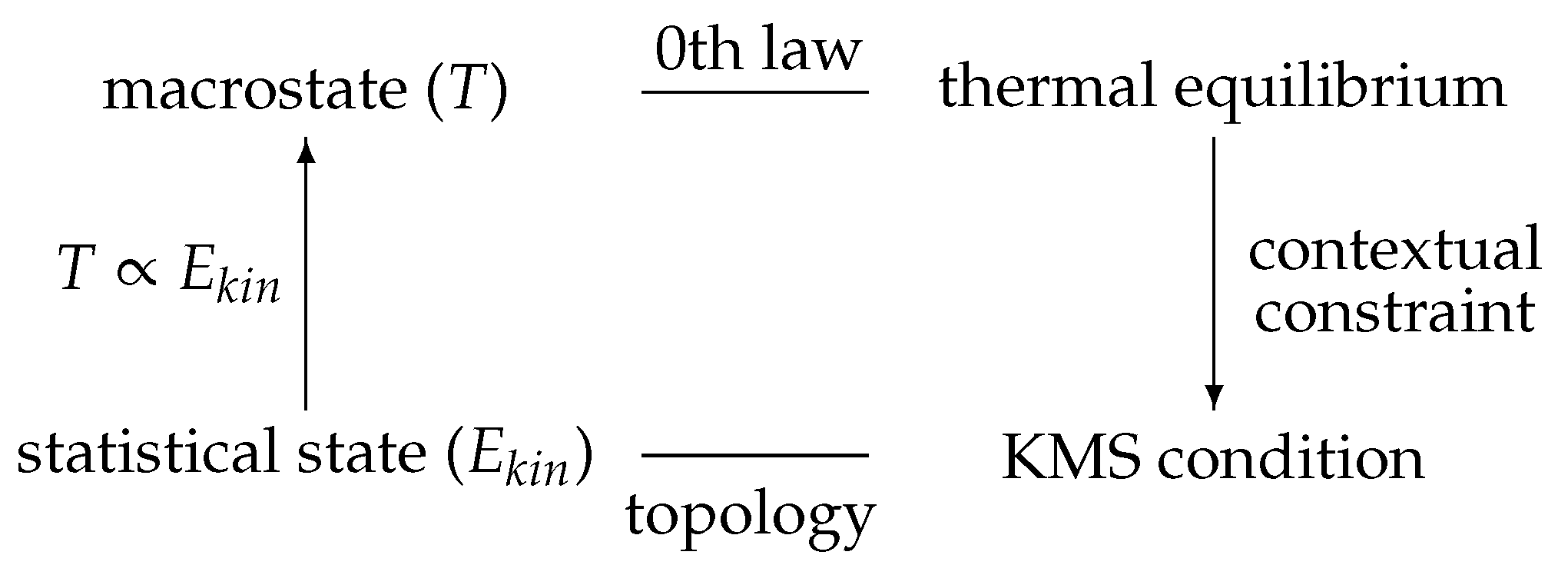
2.2. Equilibrium Macrostates: Temperature

The procedure of contextual emergence has been shown to be applicable to a number of examples from the sciences. A paradigmatic case study is the emergence of thermodynamic observables such as temperature from a mechanical description (Bishop and Atmanspacher [61]). This case is of particular interest because it was not precisely understood for a long time, and its influential philosophical interpretations (such as Nagel [68]) as a case for strong reduction have been pretty much misleading.
Step (1) in the discussion of Section 2.1 is here the step from point mechanics to statistical mechanics, essentially based on the formation of an ensemble distribution. Particular properties of a many-particle system are defined in terms of a statistical ensemble description (e.g., as moments of a many-particle distribution function), which refers to the statistical state of an ensemble ( L s ) rather than the individual states of single particles ( L i ). An example for an observable associated with the statistical state of a many-particle system is its mean kinetic energy. The expectation value of kinetic energy is defined as the limit of its mean value for infinite N.
Step (2) is the step from statistical mechanics to thermodynamics. Concerning observables, this is the step from the expectation value of a momentum distribution of a particle ensemble ( L s ) to the temperature macrostate of the system as a whole ( H i ). In many standard philosophical discussions, this step is mischaracterized by the false claim that the thermodynamic temperature of a gas is identical with the mean kinetic energy of the molecules that constitute the gas.
In Nagel’s [68] distinction of homogeneous and heterogeneous reduction, the relation between mechanics and (equilibrium) thermodynamics is heterogeneous because the descriptive terms at the two levels are different, and a “bridge law” is needed to relate them to one another. A crucial bridge law in this respect, first derived from the canonical Maxwell–Boltzmann distribution of velocities in the kinetic theory of gases in the mid-19th century, relates temperature T to the mean kinetic energy E k i n of gas particles,
E k i n = 3 2 k T ,
where k is Boltzmann’s constant. Note that the numerical equality of both sides of the equation only implies the co-extensivity of the variables, not their identity! As is well known today, the algebras of mechanical and thermodynamic observables are very different in nature.
A deeper understanding of Equation (1) was obtained a century later, when Haag and colleagues formulated statistical mechanics in the framework of algebraic quantum field theory (Haag et al. [69]). Temperature relies on the context of thermal equilibrium through the zeroth law of thermodynamics, which does not exist in statistical mechanics. However, thermal equilibrium states can be related to statistical mechanical states by a stability condition implemented onto the mechanical state space (Haag et al. [70], Kossakowski et al. [71]). This condition is the so-called KMS condition (due to Kubo, Martin and Schwinger), which can be defined by the following three points:
  • A KMS state μ is stationary (or invariant) with respect to a subset A of the state space X and with respect to a flow Φ on X, μ ( Φ 1 ( A ) ) = μ ( A ) . Then, the continuous functions assigned to μ, representing its observables, have stationary expectation values and higher statistical moments.
  • A KMS state μ is structurally stable under small perturbations of relevant parameters if it is ergodic under the flow Φ if an invariant set A has either measure oor one: μ ( A ) { 0 , 1 } (Haag et al. [70]). Otherwise, if 0 < μ ( A ) < 1 , then μ is non-ergodic and generally not structurally stable.
  • A KMS state μ has no memory of temporal correlations, i.e., it is mixing: | μ ( A ) Φ t ( B ) μ ( A ) μ ( B ) | 0 for t for all measurable subsets A and B. This can be rephrased in terms of vanishing correlations between observables (Luzzatto [72]).
The relation between a thermal equilibrium state and the KMS state provides the sound foundation for the bridge law (1) (see Remark A9).
The KMS condition induces a contextual topology, which is basically a coarse-graining of the microstate space ( L i ) that serves the definition of the states (distributions) of statistical mechanics ( L s ). This means nothing else than a partitioning of the state space into cells, leading to statistical states ( L s ) that represent equivalence classes of individual states ( L i ). They form ensembles of states that are indistinguishable with respect to their mean kinetic energy and can be assigned the same temperature ( H i ). Differences between individual microstates at L i falling into the same equivalence class at L s are irrelevant with respect to emergent macrostates with a particular temperature. Figure 2 illustrates the overall construction as a self-consistent procedure.

2.3. Non-Equilibrium Macrostates: Laser

For systems outside or even far from thermal equilibrium, the formal framework of classical thermodynamics breaks down, and thermodynamic observables typically become ill-defined. However, as has been shown in many examples, it is possible to use the mathematical structure of thermal macrostates and emergent observables as a guideline to construct analogous macrostates and emergent observables for non-equilibrium situations. A historic example, first worked out by Graham and Haken [73] and Hepp and Lieb [74], was the study of light amplification by stimulated emission of radiation (laser).
A laser is an open dissipative system consisting of a gain medium put into a cavity. As long as no external energy is pumped into the gain medium, it is simply a many-particle system in thermal equilibrium with its environment, and the randomly excited states of the particles emit radiation spontaneously. If the gain medium is pumped to a degree at which the pump power exceeds the internal cavity losses, stimulated emission of radiation kicks in, and the system establishes a highly coherent and intense radiation field within the cavity.
Below this pump threshold, the energy distribution of the microstates of the particles of the gain medium is a Boltzmann distribution, and higher-energy states stochastically relax to lower-energy states by spontaneously emitting incoherent radiation. Beyond the threshold, the relaxation becomes stimulated, to the effect that higher energy levels are more populated than lower levels (gain inversion). This drives the system away from equilibrium, and the emitted radiation is phase-correlated and coherent.
In simple cases (such as single-mode lasers), the resulting nonlinear dynamics of a radiation field coupled to a gain medium within a cavity can be described fully quantum theoretically (Ali and Sewell [75]; see also Chapter 11 in [76]). A key result is that the laser dynamics beyond the threshold instability enters an attractor, meaning that the emergent emission of coherent monochromatic radiation is stable. This stable attractor is the macrostate of the system, and its associated emergent observable is the intensity of the radiation field.
Macrostate attractors of open dissipative systems far from thermal equilibrium can be characterized by their stability against perturbations. A basic condition to be satisfied in this respect is that the sum of all Lyapunov exponents of the system is negative or, alternatively, that the divergence of the flow operator of the system is negative. If, in addition, at least one Lyapunov exponent is positive, the notion of an SRB measure (according to Sinai, Ruelle and Bowen) expresses a dynamical kind of stability analogous to KMS states. An SRB state (for hyperbolic systems) is invariant under the flow of the system for all t, and it is ergodic and mixing.
The behavior of mode intensity (or spectral power density for multimode systems) as a function of external pump power is more or less linear up to saturation (if there are no further instabilities). It can be understood as the efficiency of the lasing activity, which is analogous to specific heat in thermal equilibrium. In the same sense, the laser threshold instability is analogous to a second-order phase transition, where radiation intensity grows continuously, but its derivative, efficiency, does not.
Further increase of the pump power, particularly in multimode lasers, may lead to further instabilities, such as higher-dimensional chaotic attractors (Haken [77]). Experimental work by Atmanspacher and Scheingraber [78] demonstrated a sequence of such instabilities in multimode lasers. These results will be discussed in more detail in Section 4.3, where the different behavioral regimes of multimode lasers will be related to the concept of pragmatic information.

3. Partitions Based on Dynamics

3.1. Generating Partitions

The concept of a generating partition is of utmost significance in the ergodic theory of dynamical systems (Cornfeld et al. [79]) and in the field of symbolic dynamics (Lind and Marcus [35]). It is tightly related to the dynamical entropy of a system with respect to both its dynamics Φ : X X and a partition P (Cornfeld et al. [80]):
H ( Φ , P ) = lim n 1 n H ( P Φ 1 ( P ) Φ n ( P ) ) .
In other words, this is the limit of the entropy of the product of partitions of increasing dynamical refinement.
A special case of a dynamical entropy of the system with dynamics Φ is the Kolmogorov–Sinai entropy (Kolmogorov [57], Sinai [81]):
H K S = sup P H ( Φ , P ) .
This supremum over all partitions P is assumed if P is a generating partition P g , otherwise H ( Φ , P ) < H K S . P g minimizes correlations among partition cells A i , so that only correlations due to Φ itself contribute to H ( Φ , P g ) , and the partition is stable under Φ. Boundaries of A i are (approximately) mapped onto one another. Spurious correlations due to blurring cells are excluded, so that the dynamical entropy takes on its supremum.
The Kolmogorov–Sinai entropy is a key property of chaotic systems, whose behavior depends sensitively on initial conditions. This dependence is due to an intrinsic instability that is formally reflected by the existence of positive Lyapunov exponents. The KS-entropy is essentially given by the sum of those positive Lyapunov. A positive (finite) KS-entropy is a necessary and sufficient condition for chaos in conservative, as well as in dissipative systems (with a finite number of degrees of freedom). Chaos in this sense covers the range between totally unpredictable random processes, such as white noise ( H K S ), and regular (e.g., periodic, etc.) processes with H K S = 0 .
The concept of a generating partition in the ergodic theory of deterministic systems is related to the concept of a Markov chain in the theory of stochastic systems. Every deterministic system of first order gives rise to a Markov chain, which is generally neither ergodic, nor irreducible. Such Markov chains can be obtained by so-called Markov partitions that exist for hyperbolic dynamical systems (Sinai [82], Bowen [83], Ruelle [84]). For non-hyperbolic systems, no corresponding existence theorem is available, and the construction can be even more tedious than for hyperbolic systems (Viana et al. [85]). For instance, both Markov and generating partitions for nonlinear systems are generally non-homogeneous, i.e., their cells are typically of different sizes and forms (see Remark A10).
Since the cells of a generating partition are dynamically stable, they can be used to define dynamically-stable symbolic macrostates s (see Remark A11), whose sequence provides a symbolic dynamics σ (Lind and Marcus [35]). This dynamics of macrostates is a faithful representation of the underlying dynamics Φ of microstates x only for generating partitions. More formally, the dynamics Φ and σ are related to each other by:
π Φ = σ π ,
where π acts as an intertwiner, which can be represented diagrammatically as:
Entropy 18 00426 i001
If π is continuous and invertible and its inverse π 1 is also continuous, the maps Φ and σ are topologically equivalent. For generating partitions, the correspondence between the space of microstates and its macrostate representation is one-to-one: each point in the space of microstates is uniquely represented by a bi-infinite symbolic sequence and vice versa. In addition, all topological information is preserved.

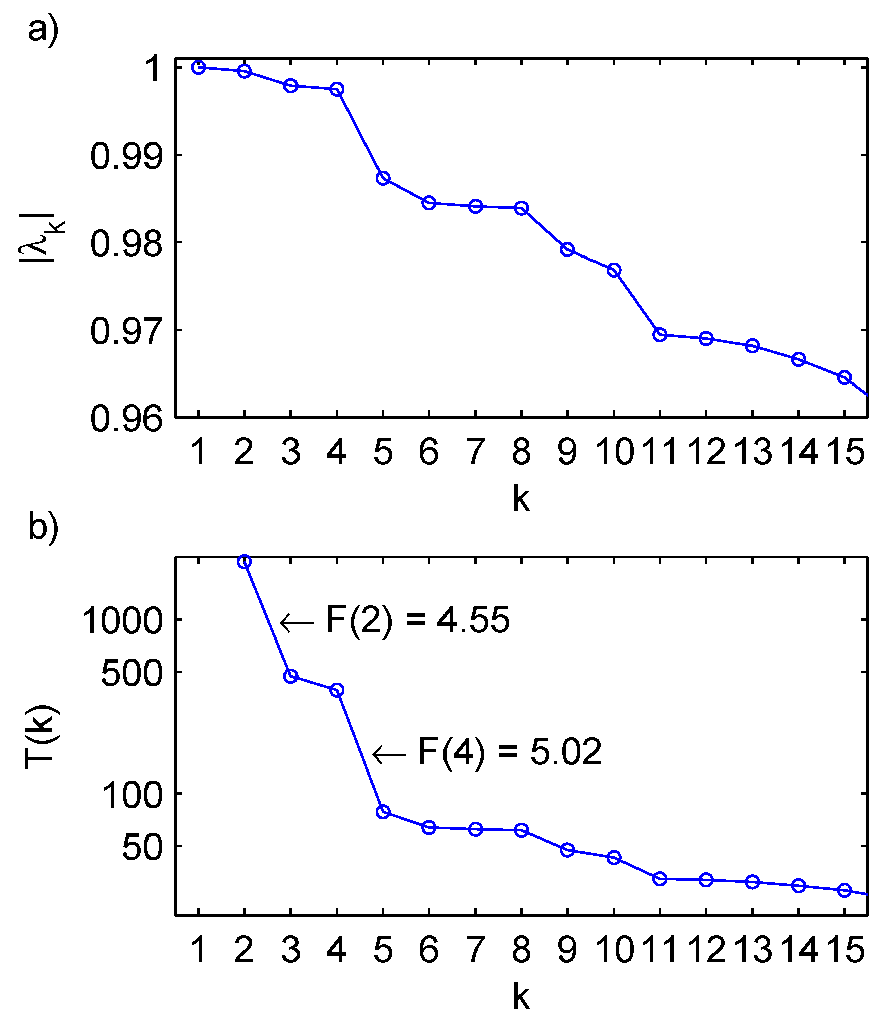
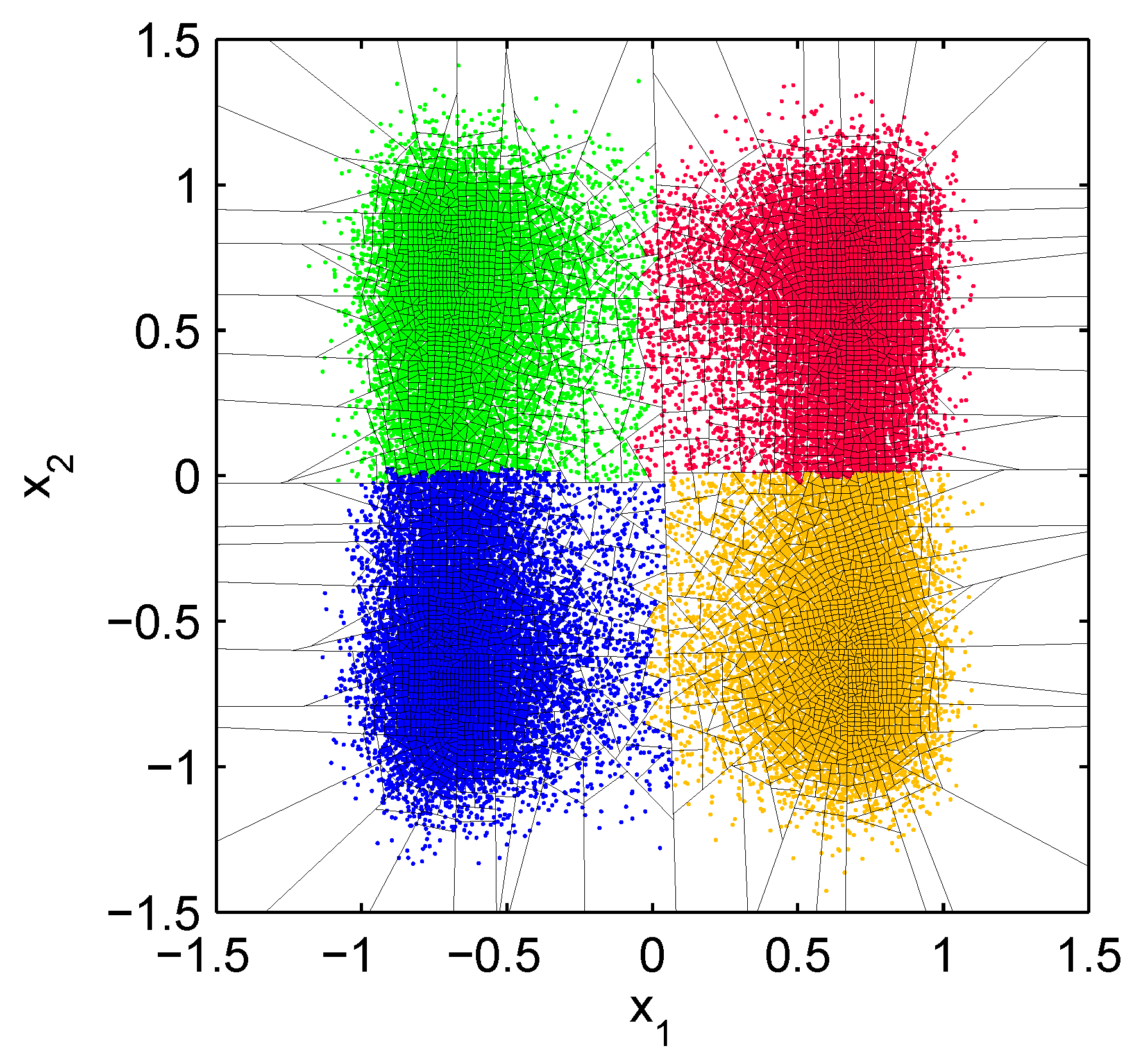
3.2. Almost Invariant Sets as Macrostates

Macrostates correspond to the “almost invariant sets” (Froyland [66]) of a dynamical system, i.e., subsets of the state space that are approximately invariant under the system’s dynamics. For a given dynamics, these subsets can be identified by a partitioning procedure developed by Allefeld et al. [86], which relies on work by Deuflhard and Weber [87], Gaveau and Schulman [65] and Froyland [66]. The present subsection sketches how this procedure works for numerically-simulated data, while the next subsection addresses its application to empirical data (see Remark A12).
The simulated system is a discrete-time stochastic process in two dimensions, ( x 1 , x 2 ) , where the change at each time step is given by:
Δ x i = a x i 2 x i 3 + b i ξ i , i = 1 , 2 .
The first term describes an overdamped motion within a double-well potential along each dimension, leading to four attracting points at ( x 1 , x 2 ) = ( ± 2 , ± 2 ) . The second, stochastic term generates a random walk, so that the system occasionally moves from one into another point’s basin of attraction. These switches occur more frequently along the second dimension because the noise amplitude is larger in that direction, b 2 > b 1 . Figure 3 shows the state space of this multistable system and a suitable microstate partition (see Allefeld et al. [86] for details).
Counting the transition between microstates leads to an estimate of the transition matrix R. Since the existence of q almost invariant sets leads to q largest eigenvalues λ k , gaps in the eigenvalue spectrum are a natural candidate to estimate the number of macrostates directly from the given data. However, the concrete eigenvalues in the spectrum of R depend on the timescales. Therefore, the eigenvalues are transformed into associated characteristic timescales,
T ( k ) = 1 log | λ k | ,
and a timescale separation factor can be introduced as the ratio of subsequent timescales:
F ( k ) = T ( k ) T ( k + 1 ) = log | λ k + 1 | log | λ k | .
F ( k ) provides a measure of the spectral gap between eigenvalues λ k and λ k + 1 that is independent of the timescale.
The largest eigenvalues of R are plotted in Figure 4a, revealing a group of four leading eigenvalues (>0.995), which is subdivided into two groups of two eigenvalues each. This becomes clearer after the transformation into timescales T ( k ) . In Figure 4b, they are displayed on a logarithmic scale, such that the magnitude of timescale separation factors F ( k ) is directly apparent in the vertical distances between subsequent data points. The largest separation factors indicate that a partitioning of the state space into four macrostates is optimal, while two different macrostates may also be meaningful.
The identification of almost invariant sets of microstates defining macrostates is performed within the three-dimensional eigenvector space ( o 1 , o 2 , o 3 ) . Figure 5 reveals that the points representing microstates are located on a saddle-shaped surface stretched out within a four-simplex. Identifying the vertices of the simplex, one can attribute each microstate to that macrostate whose defining vertex is closest, resulting in the depicted separation into four sets.
In Figure 6, this result is re-translated into the original state space of Figure 3, by coloring the data points of each microstate according to the macrostate to which it is assigned. The identified macrostates coincide with the basins of attraction of the four attracting points of the system given in (5).
From Figure 5, one can also assess which macrostate definitions would be obtained by choosing q = 2 , the next-best choice for the number of macrostates according to the timescale separation criterion. In this case, the eigenvector space is spanned by the single dimension o 1 , along which the two vertices of the four-simplex on the left and right side, respectively, coincide. This means that the two resulting macrostates each consist of the union of two of the macrostates obtained for q = 4 . With respect to the state space, these two macrostates correspond to the domains x 1 > 0 and x 1 < 0 .
This can be easily understood since, because of the smaller probability of transitions along x 1 ( b 2 > b 1 ), these two areas of the state space form almost invariant sets, as well. As can be seen from this example, the possibility to select different q-values of comparably good rating allows us to identify different dynamical levels of a system, which give rise to a hierarchical structure of potential macrostate definitions.

3.3. Mental Macrostates from Neurodynamics

In this subsection, we give an example, where the described procedure has been established for empirical data. The descriptive levels studied here are those of neural microstates and mental macrostates, far less precisely defined than micro-and macrostates in physical situations. Nevertheless, it will be demonstrated that stable and relevant macrostates can be identified along the lines sketched above.
Let us assume a (lower level) neural state space X with fine-grained states x, ideally represented pointwise in X and with observables X i , i = 1 , , n , for n degrees of freedom. Typical examples for neural observables are electroencephalogram (EEG) potentials, local field potentials or even spike trains of neurons. These observables are usually obtained with higher resolution than can be expected for observables at a mental level of description.
The construction of a (higher level) mental state space Y from X requires some coarse-graining of X. That is, the state space X must be partitioned, such that cells of finite volume in X emerge, which eventually can be used to represent mental states in Y. Such discrete macrostates can be denoted by symbols A , B , C , , where each symbol represents an equivalence class of neural states. In contrast to the (quasi-)continuous dynamics of states x in a state space X, the symbolic dynamics in Y is a discrete sequence of macrostates as a function of time.
A coarse-grained partition on X implies neighborhood relations between statistical states in X (which can then be identified as mental macrostates in Y) that are different from those between individual microstates in X; in this sense, it implies a change in topology. Moreover, the observables Y i for Y belong to an algebra of mental observables that is different from that of neural observables. Obviously, these two differences depend essentially on the choice of the partition of X.
First of all, it should be required that a proper partition leads to mental states in Y that are empirically plausible. For instance, one plausible formation of basic equivalence classes of neural states is due to the distinction between wakefulness and sleep; two evidently different mental states. However, an important second demand is that these equivalence classes be stable under the dynamics in X. If this cannot be guaranteed, the boundaries between cells in X become blurred as time proceeds, thus rendering the concept of a mental state ill-defined. Atmanspacher and beim Graben [88] showed in detail that generating partitions are needed for a proper definition of stable states in Y based on cells in X.
A pertinent example for the successful application of this idea to experimental data was worked out by Allefeld et al. [86], using EEG data from subjects with sporadic epileptic seizures. This means that the neural level is characterized by brain states recorded via EEG. The context of normal versus epileptic mental states essentially requires a bipartition of the neural state space in order to identify the corresponding mental macrostates.
The data analytic procedure is the same as described in Section 3.2 for the numerically study of a multistable system with four macrostates. It starts with a 20-channel EEG recording, giving rise to a state space of dimension 20, which can be reduced to a lower number by restricting to principal components. On the resulting low-dimensional state space, a homogeneous grid of cells is imposed in order to set up a Markov transition matrix R reflecting the EEG dynamics on a fine-grained auxiliary microstate partition.
The eigenvalues of this matrix yield characteristic timescales T for the dynamics, which can be ordered by size. Gaps between successive timescales indicate groups of eigenvectors defining partitions of increasing refinement; usually, the largest timescales can be regarded most significant for the analysis. The corresponding eigenvectors together with the data points belonging to them define the neural state space partition relevant for the identification of mental macrostates.
Finally, the result of the partitioning can be inspected in the originally recorded time series to check whether mental states are reliably assigned to the correct episodes in the EEG dynamics. The study by Allefeld et al. [86] shows good agreement between the distinction of macrostates pertaining to normal and epileptic episodes and the bipartition resulting from the spectral analysis of the neural transition matrix.
As mentioned in Section 3.1, an important feature of dynamically-stable (i.e., generating) partitions is the topological equivalence of representations at lower and higher levels. Metzinger [89] (p. 619) and Fell [90] gave empirically-based examples for neural and mental state spaces in this respect. Non-generating partitions provide representations in Y that are topologically inequivalent and, hence, incompatible with the underlying representation in X. Conversely, compatible mental models that are topologically equivalent with their neural basis emerge if they are constructed from generating partitions.
In this spirit, mental macrostates constructed from generating partitions were recently shown to contribute to a better understanding of a long-standing puzzle in the philosophy of mind: mental causation. The resulting contextual emergence of mental states dissolves the alleged conflict between the horizontal (mental-mental) and vertical (neural-mental) determination of mental events as ill-conceived (Harbecke and Atmanspacher [91]). The key point is a construction of a properly-defined mental dynamics topologically equivalent with the dynamics of underlying neural states. The statistical neural states based on a proper partition are then coextensive (but not identical) with individual mental states.
As a consequence: (i) mental states can be horizontally-causally related to other mental states; and (ii) they are neither causally related to their neural determiners, nor to the neural determiners of their horizontal effects. This makes a strong case against a conflict between a horizontal and a vertical determination of mental events and resolves the problem of mental causation in a deflationary manner. Vertical and horizontal determination do not compete, but complement one another in a cooperative fashion (see Remark A13).

4. Meaningful Macrostates

4.1. Stability and Relevance

As repeatedly emphasized above, not every arbitrarily-chosen partition of a microstate space provides macrostates that make sense for the system at higher levels of description. Stability criteria can be exploited to distinguish proper from improper partitions, such as the KMS condition for thermal systems or the concept of generating partitions for nonlinear dynamical systems, especially if they are hyperbolic.
Insofar as the required stability criteria derive from a higher level context, they implement information about cooperative higher level features of the system at its lower descriptive level. This, in turn, endows the lower level with a new contextual topology defined by a partition into equivalence classes of microstates. Differences between microstates in the same equivalence class are irrelevant with respect to the higher level context, at which macrostates are to be identified. In this sense, the stability criterion applied is at the same time a relevance criterion.
Yet, groups of macrostates of different degrees of coarseness may result from the spectral analysis. As discussed in Section 3.2, the four coexisting basins of attraction of the system considered yield two partitions, one of which is a refinement of the other. The relevance of the corresponding levels, or scales, of macrostates in this example is known by construction, i.e., due to different amounts of noise causing different transition probabilities between the basins.
A similar feature was found in the example of EEG data discussed in Section 3.3. The distinction of epileptic seizures versus normal states clearly sets the context for a bipartition of the space of microstates. However, it would be surprising if the “normal” state, extending over long periods of time, would not show additional fine structure. Indeed, the timescale analysis (see details in Allefeld et al. [86]) shows a second plateau after the first two eigenvalues, indicating such a fine structure within the normal state. Since, in this example, no information about the context of this fine structure is available, the relevance of the corresponding “mesoscopic” states remains unclarified.
At a more general level, the relevance problem pervades any kind of pattern detection procedure, and it is not easy to solve. This is particularly visible in the trendy field of “data mining and knowledge discovery” (Fayyad et al. [92], Aggarwal [93]), a branch of the equally trendy area of “big-data science”, with its promises to uncover new science purely inductively from very large databases. Pure induction in this sense is equivalent to the construction of macrostates (patterns) from microstates (data points) without any guiding context. Of course, this is possible, but questions concerning the stability and relevance of such macrostates cannot be reasonably addressed without additional knowledge or assumptions.
Without contextual constraints, most macrostates constructed this way will be spurious in the sense that they are not meaningful. A nice illustration of the risk of misleading ideas of context-free pattern detection is due to Calude and Longo [94]. Using Ramsey theory, they show that in very large databases, most of the patterns (correlations) identified must be expected to be spurious. The same problem has recently been emphasized by the distinction between statistical and substantive significance in multivariate statistics. Even an extremely low probability (p-value) for a null hypothesis to be found by chance does not imply that the tested alternative hypothesis is meaningful (see Miller [95]).
In a very timely and concrete sense, meaningful information over and above pure syntax plays a key role in a number of approaches in the rapidly developing field of semantic information retrieval as used in semantic search algorithms for databases (see Remark A14). Many such approaches try to consider the context of lexical items by similarity relations, e.g., based on the topology of these items (see, e.g., Cilibrasi and Vitànyi [96]). This pragmatic aspect of meaning is also central in situation semantics on which some approaches of understanding meaning in computational linguistics are based (e.g., Rieger [97]).

4.2. Meaningful Information and Statistical Complexity

Grassberger [54] and Atlan [98] were the first to emphasize a close relationship between the concepts of complexity and meaning. For instance, Grassberger (his italics) wrote [44]:
Complexity in a very broad sense is a difficulty of a meaningful task. More precisely, the complexity of a pattern, a machine, an algorithm, etc. is the difficulty of the most important task related to it. . . . As a consequence of our insistence on meaningful tasks, the concept of complexity becomes subjective. We really cannot speak of the complexity of a pattern without reference to the observer. . . . A unique definition (of complexity) with a universal range of applications does not exist. Indeed, one of the most obvious properties of a complex object is that there is no unique most important task related to it.
Although this remarkable statement by one of the pioneers of complexity research in physics dates almost 30 years back from now, it is still a challenge to understand the relation between the complexity of a pattern or a symbol sequence and the meaning that it can be assigned in detail.
Already Weaver’s contribution in the seminal work by Shannon and Weaver [24] indicated that the purely syntactic component of information today known as Shannon information requires extension into semantic and pragmatic domains. If the meaning of some input into a system is understood, then it triggers action and changes the structure or behavior of the system. In this spirit, Weizsäcker [99] introduced a way of dealing with the use a system makes of some understood meaning of an input (e.g., a message) in terms of pragmatic information.
Pragmatic information is based on the notions of novelty and confirmation. Weizsäcker argued that a message that does nothing but confirm the prior knowledge of a system will not change its structure or behavior. On the other hand, a message providing (novel) material completely unrelated to any prior knowledge of the system will not change its structure or behavior either, simply because it cannot be understood. In both cases, the pragmatic information of the message vanishes. A maximum of pragmatic information is acquired if an optimal combination of novelty and confirmation is transferred to the system.
Based on pragmatic information, an important connection between meaning and complexity can be established (cf. Atmanspacher [52]). A checkerboard-like period-two pattern, which is recurrent after the first two steps (compare Figure 1 left), is a regular pattern of small complexity, for both monotonic (deterministic) and convex (statistical) definitions of complexity as introduced in Section 1.2. Such a pattern does not yield additional meaning as soon as the initial transient phase is completed.
For a maximally random pattern, monotonic (deterministic) complexity and convex (statistical) complexity lead to different assessments. Deterministically, a random pattern can only be represented by an incompressible algorithm with as many steps as the pattern has elements. A representation of the pattern has no recurrence at all within the length of the representing algorithm. This means that it never ceases to produce elements that are unpredictable. Hence, the representation of a random pattern can be interpreted as completely lacking confirmation and consequently with vanishing meaning.
If the statistical notion of complexity is focused on, the pattern representation is no longer related to the sequence of individually distinct elements. A statistical representation of the pattern is not unique with respect to its local properties; it is characterized by a global statistical distribution (see Remark A15). This entails a significant shift in perspective. While monotonic complexity relates to syntactic information as a measure of randomness, the convexity of statistical complexity coincides with the convexity of pragmatic information as a measure of meaning (see Figure 7).

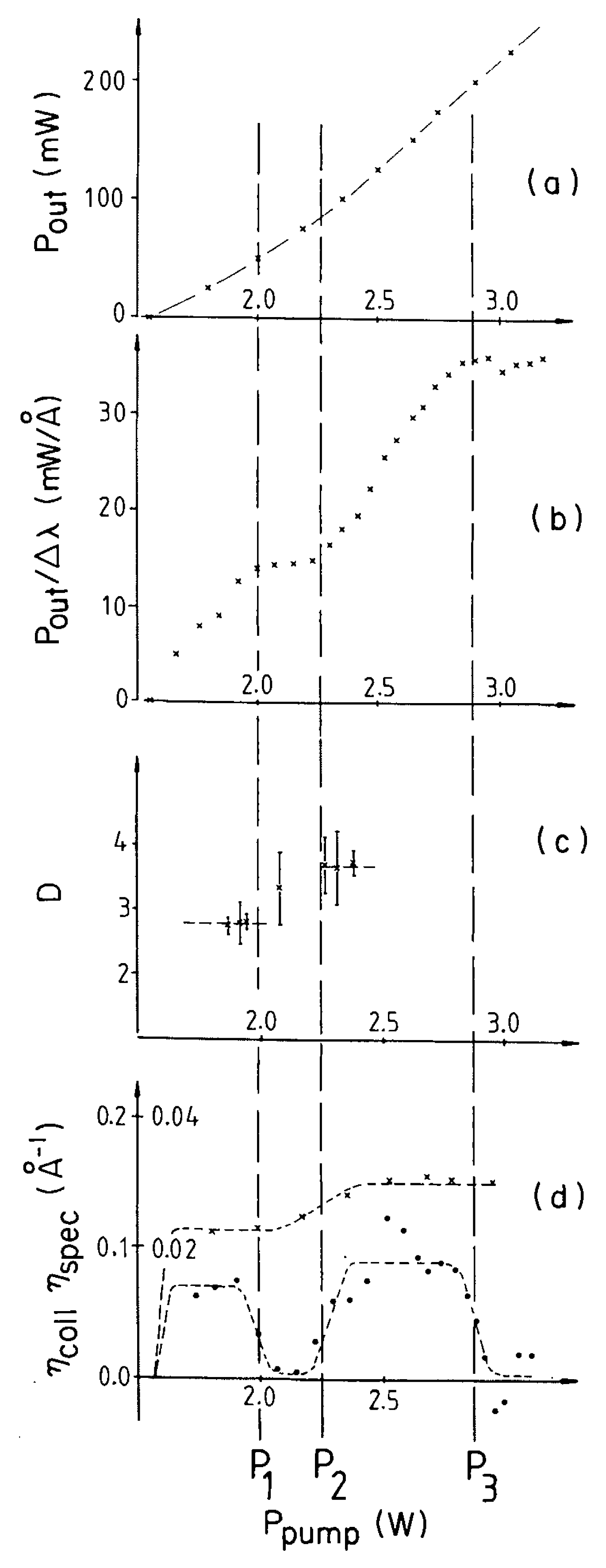
4.3. Pragmatic Information in Non-Equilibrium Systems

Although the notions of meaning and its understanding are usually employed in the study of cognitive systems, also physical systems allow (though not require) a description in terms of pragmatic information. This has been shown by Atmanspacher and Scheingraber [100] for the example discussed in Section 2.3: laser systems far from thermal equilibrium. Instabilities in such laser systems can be considered as meaningful in the sense of positive pragmatic information if they are accompanied by a structural change of the system’s self-organized behavior. We conclude this paper with a brief review of the results of this work (for details, see the original publication).
As mentioned in Section 2.3, key macro-quantities for laser systems are the input power P p u m p , the output power P o u t and (for multimode lasers with bandwidth Δ λ ) its spectral density P o u t / Δ λ . The gradient of output versus input power is the collective efficiency:
η c o l l = d P o u t / d P p u m p ,
and the spectral output yields a specific efficiency according to:
η s p e c = d P o u t / d P p u m p Δ λ .
The efficiencies are crucial for a first and rough definition of the pragmatic information that is released during instabilities at critical values of P p u m p . For an initial efficiency η i below an instability and a final efficiency η f beyond an instability, one can define a normalized pragmatic information P I for the system by:
P I = η f η i η f
Figure 8 shows these properties as a function of input (pump) power. Below the laser threshold, where P o u t = 0 , the system is in thermal equilibrium with a temperature that can be estimated by the population density in the energy levels of the gain medium. Hence, the thermodynamic entropy is maximal and the efficiencies according to (8) and (9) are zero. Above the threshold, the laser is in a non-equilibrium state (gain inversion), and its efficiency after the threshold instability is η f > 0 . Consequently, the pragmatic information (10) released at the threshold instability is P I = η f / η f = 1 .
Figure 8b shows that the spectral power density increases up to P 1 and, in contrast to P o u t in Figure 8a, stays more or less constant between P 1 and P 2 . Beyond P 2 , it rises again, and beyond P 3 , it stays constant again. The two plateaus arise due a simultaneous growth of P o u t and emission bandwidth Δ λ . Figure 8c shows the so-called correlation dimension D, a measure of the number of macroscopic degrees of freedom of the system (see Remark A16). It changes between P 1 and P 2 , indicating a structural change of the attractor of the system dynamics and, thus, a switch between two types of stable self-organized behavior that can be understood by mode coupling mechanisms within the intracavity radiation field (for details, see Atmanspacher and Scheingraber [100]).
This structural change is related to changes of the efficiencies (Equations (8) and (9)) in Figure 8d, which are derived as the local gradients of output power and spectral output power versus pump power. Collective efficiency increases at the laser threshold and between P 1 and P 2 , as it should for the analog of second-order phase transitions (cf. Section 2.3). However, the behavior of specific efficiency is different: it increases at the threshold, decreases by the same amount at P 1 , then grows to a larger value at P 2 and drops again at about P 3 . Pragmatic information according to (10) behaves qualitatively the same way.
At the laser threshold, where self-organized behavior far from equilibrium in terms of stimulated emission of coherent light emerges, pragmatic information is released. The system “understands” the onset of self-organized cooperative behavior and adapts to it by acting according to new constraints. At input powers between P 1 and P 2 , another structural change occurs, which essentially effects the phase relations between individual laser modes. Since D increases by about one between P 1 and P 2 , it is tempting to assume that these modes, coherently oscillating as one group below P 1 , split up into two decoupled groups of coupled modes beyond P 2 . If the input power is further increased, the system can show more instabilities. For very high pump powers, D falls back to values between two and three as between the laser threshold and P 1 .
A final remark: talking about a physical system releasing and understanding meaning, which then turns into an urge for action to re-organize its behavior, does not imply that such systems have mental capacities, such as perception, cognition, intention, or the like. However, models of mental activity, such as small-world or scale-free networks, which are currently popular tools in cognitive neuroscience, offer themselves to employ interpretations in terms of pragmatic information in a more direct fashion (see Remark A17).

Acknowledgments

Thanks to Carsten Allefeld and Jiri Wackermann for their permission to use material from Allefeld et al. [86] in this paper. I am also grateful to three anonymous referees for helpful comments.

Conflicts of Interest

The author declares no conflict of interest.

Appendix A

Remark A1.
This is evident in measurements of quantum systems. A key feature of quantum measurement is that successive measurements generally do not commute. This is due to a backreaction of the measurement process on the state of the system, which has also been discussed for complex systems outside quantum physics, in particular for cognitive systems (Busemeyer and Bruza [101]).
Remark A2.
Note that deterministic measures are not free from statistical elements. The point of this distinction is that individual accounts are delineated from ensemble accounts.
Remark A3.
It should be emphasized that randomness itself is a concept that is anything else than finally clarified. Here, we use the notion of randomness in the broad sense of entropy.
Remark A4.
Informative discussions of various types of emergent versus reductive inter-level relations are due to Beckermann et al. [102], Gillett [103], Butterfield [104] and Chibbaro et al. [105].
Remark A5.
Mathematically, an equivalence class with respect to an element a of a set X is the subset [ a ] of all elements x X satisfying an equivalence relation “∼”: [ a ] = { x X | a x } . A property F ( x ) defines an equivalence relation if and only if F ( x i ) = F ( x j ) for x i x j .
Remark A6.
Note that this step (1) is also crucial for the so-called GNS-representation (due to Gel’fand, Naimark and Segal) of states in algebraic quantum theory. This representation requires the (contextual) choice of a reference state in the space of individual states (the dual A * of the basic C*-algebra A of observables), which entails a contextual topology giving rise to statistical states (in the predual M * of the corresponding W*-algebra M of observables. If the algebra is purely non-commutative (as in traditional quantum mechanics), A * is isomorphic to M * , so that there is a one-to-one correspondence between individual states and (extremal) statistical states. In the general case of an algebra containing both commuting and non-commuting observables, the statistical states in M * are equivalence classes of individual states in A * . For details, see the illuminating discussion by Primas [106].
Remark A7.
As an alternative to stability considerations, it is possible to use a general principle of maximum information (Haken [14]) to find stable states in complex systems under particular constraints. In equilibrium thermodynamics, this principle reduces to the maximum entropy condition for thermal equilibrium states. In the present contribution, we will mostly restrict ourselves to stability issues as criteria for proper partitions.
Remark A8.
In the terminology of synergetics (Haken [14]), the contextually-emergent observables are called order parameters, and the downward constraint that they enforce upon the microstates is called slaving. Order parameters need to be identified contextually, depending on the higher-level description looked for, and cannot be uniquely derived from the lower-level description that they constrain.
Remark A9.
For a good overview and more details see Sewell (Chapters 5 and 6) [76]. Alternatively, KMS states can be interpreted as local restrictions of the global vacuum state of quantum field theory within the Tomita–Takesaki modular approach, as Schroer [107] pointed out; see also Primas (Chapter 7) [108] for further commentary. This viewpoint beautifully catches the spirit of the role of downward confinement in contextual emergence.
Remark A10.
Every Markov partition is generating, but the converse is not necessarily true (Crutchfield and Packard [109]). For the construction of “optimal” partitions from empirical data, it is often convenient to approximate them by Markov partitions (Froyland [66]); see the following subsections.
Remark A11.
There are possibilities to construct stable partitions in information theoretical terms, as well. For instance, in computational mechanics (Shalizi and Crutchfield [37]), all past microstates leading to the same prediction (up to deviations of size ϵ) about the future of a process form an equivalence class called a causal state. These states are macrostates. Together with the dynamics, they can be used to construct a so-called ϵ-machine, which is an optimal, minimal and unique predictor of the system’s behavior.
Remark A12.
A number of technical details will be omitted in this presentation. Interested readers should consult the original paper by Allefeld et al. [86].
Remark A13.
This argument was less formally put forward by Yablo [110]. A recent paper by Hoel et al. [111] makes a similar point based on the identification of different spatiotemporal neural/mental scales in the framework of integrated information theory.
Remark A14.
For an early reference, see Amati and van Rijsbergen [112]; a recent collection of essays is due to de Virgilio et al. [113]. The semantic web (web 3.0, linked open data, web of data) due to Berners-Lee et al. [114] is an obviously related development.
Remark A15.
A closer look into the definitions of statistical complexity measures shows that their two-level structure (see Section 1.2) actually accounts for a subtle interplay of local and global properties. For instance, variance complexity (Atmanspacher et al. [60]) is the global variance of local (block) variances based on suitably chosen partitions (blocks) of the data forming the pattern.
Remark A16.
The dimension D of an attractor is the dimension of the subspace of its macroscopic state space that is required to model its behavior. An algorithm due to Grassberger and Procaccia [115] can be used to determine D from empirical time series of the system.
Remark A17.
For some corresponding ideas concerning learning in networks, see Atmanspacher and Filk [116] or, for an alternative approach, Crutchfield and Whalen [117]. Moreover, see Freeman [118] for an interesting application of the concept of pragmatic information in the interpretation of EEG dynamics.

References

  1. Cowan, G.A.; Pines, D.; Meltzer, D. (Eds.) Complexity—Metaphors, Models, and Reality; Addison-Wesley: Reading, MA, USA, 1994.
  2. Cohen, J.; Stewart, I. The Collapse of Chaos; Penguin: New York, NY, USA, 1994. [Google Scholar]
  3. Auyang, S.Y. Foundations of Complex-System Theories; Cambridge University Press: Cambridge, UK, 1998. [Google Scholar]
  4. Scott, A. (Ed.) Encyclopedia of Nonlinear Science; Routledge: London, UK, 2005.
  5. Shalizi, C.R. Methods and techniques of complex systems science: An overview. In Complex System Science in Biomedicine; Dreisboeck, T.S., Kresh, J.Y., Eds.; Springer: Berlin/Heidelberg, Germany, 2006; pp. 33–114. [Google Scholar]
  6. Gershenson, C.; Aerts, D.; Edmonds, B. (Eds.) Worldviews, Science, and Us: Philosophy and Complexity; World Scientific: Singapore, 2007.
  7. Nicolis, G.; Nicolis, C. Foundations of Complex Systems; World Scientific: Singapore, 2007. [Google Scholar]
  8. Mitchell, M. Complexity: A Guided Tour; Oxford University Press: Oxford, UK, 2009. [Google Scholar]
  9. Hooker, C. (Ed.) Philosophy of Complex Systems; Elsevier: Amsterdam, The Netherlands, 2011.
  10. Von Bertalanffy, L. General System Theory; Braziller: New York, NY, USA, 1968. [Google Scholar]
  11. Wiener, N. Cybernetics, 2nd ed.; MIT Press: Cambridge, UK, 1961. [Google Scholar]
  12. Von Foerster, H. Principles of Self-Organization; Pergamon: New York, NY, USA, 1962. [Google Scholar]
  13. Mandelbrot, B.B. The Fractal Geometry of Nature, 3rd ed.; Freeman: San Francisco, CA, USA, 1983. [Google Scholar]
  14. Haken, H. Synergetics; Springer: Berlin/Heidelberg, Germany, 1983. [Google Scholar]
  15. Nicolis, G.; Prigogine, I. Self-Organization in Non-Equilibrium Systems; Wiley: New York, NY, USA, 1977. [Google Scholar]
  16. Maturana, H.; Varela, F. Autopoiesis and Cognition; Reidel: Boston, MA, USA, 1980. [Google Scholar]
  17. Hopcroft, J.E.; Ullmann, J.D. Introduction to Automata Theory, Languages, and Computation; Addison-Wesley: Reading, MA, USA, 1979. [Google Scholar]
  18. Wolfram, S. Theory and Applications of Cellular Automata; World Scientific: Singapore, 1986. [Google Scholar]
  19. Albert, R.; Barabási, A.-L. Statistical mechanics of complex networks. Rev. Modern Phys. 2002, 74, 47–97. [Google Scholar] [CrossRef]
  20. Boccaletti, S.; Latora, V.; Moreno, Y.; Chavez, M.; Hwang, D.U. Complex networks: Structure and dynamics. Phys. Rep. 2006, 424, 175–308. [Google Scholar] [CrossRef]
  21. Newman, M.; Barabási, A.; Watts, D. The Structure and Dynamics of Networks; Princeton University Press: Princeton, NJ, USA, 2006. [Google Scholar]
  22. Ali, S.A.; Cafaro, C.; Kim, D.-H.; Mancini, S. The effect of microscopic correlations on the information geometric complexity of Gaussian statistical models. Physica A 2010, 389, 3117–3127. [Google Scholar] [CrossRef]
  23. Cafaro, C.; Mancini, S. Quantifying the complexity of geodesic paths on curved statistical manifolds through information geometric entropies and Jacobi fields. Physica D 2011, 240, 607–618. [Google Scholar] [CrossRef]
  24. Shannon, C.E.; Weaver, W. The Mathematical Theory of Communication; University of Illinois Press: Urbana, IL, USA, 1949. [Google Scholar]
  25. Zurek, W.H. (Ed.) Complexity, Entropy, and the Physics of Information; Addison-Wesley: Reading, MA, USA, 1990.
  26. Atmanspacher, H.; Scheingraber, H. (Eds.) Information Dynamics; Plenum: New York, NY, USA, 1991.
  27. Kornwachs, K.; Jacoby, K. (Eds.) Information—New Questions to a Multidisciplinary Concept; Akademie: Berlin, Germany, 1996.
  28. Marijuàn, P.; Conrad, M. (Eds.) Proceedings of the Conference on Foundations of Information Science, from computers and quantum physics to cells, nervous systems, and societies, Madrid, Spain, July 11–15, 1994. BioSystems 1996, 38, 87–266. [PubMed]
  29. Boffetta, G.; Cencini, M.; Falcioni, M.; Vulpiani, A. Predictability—A way to characterize complexity. Phys. Rep. 2002, 356, 367–474. [Google Scholar] [CrossRef]
  30. Crutchfield, J.P.; Machta, J. Introduction to Focus Issue on “Randomness, Structure, and Causality: Measures of Complexity from Theory to Applications”. Chaos 2011, 21, 03710. [Google Scholar] [CrossRef] [PubMed]
  31. Stewart, I. Does God Play Dice? Penguin: New York, NY, USA, 1990. [Google Scholar]
  32. Lasota, A.; Mackey, M.C. Chaos, Fractals, and Noise; Springer: Berlin/Heidelberg, Germany, 1995. [Google Scholar]
  33. Kaneko, K. (Ed.) Theory and Applications of Coupled Map Lattices; Wiley: New York, NY, USA, 1993.
  34. Kaneko, K.; Tsuda, I. Complex Systems: Chaos and Beyond; Springer: Berlin/Heidelberg, Germany, 2000. [Google Scholar]
  35. Lind, D.; Marcus, B. Symbolic Dynamics and Coding; Cambridge University Press: Cambridge, UK, 1995. [Google Scholar]
  36. Bak, P. How Nature Works: The Science of Self-Organized Criticality; Copernicus: New York, NY, USA, 1996. [Google Scholar]
  37. Shalizi, C.R.; Crutchfield, J.P. Computational mechanics: Pattern and prediction, structure and simplicity. J. Stat. Phys. 2001, 104, 817–879. [Google Scholar] [CrossRef]
  38. Cafaro, C.; Ali, S.A.; Giffin, A. Thermodynamic aspects of information transfer in complex dynamical systems. Phys. Rev. E 2016, 93, 022114. [Google Scholar] [CrossRef] [PubMed]
  39. Solomonoff, R.J. A formal theory of inductive inference. Inf. Control 1964, 7, 224–254. [Google Scholar] [CrossRef]
  40. Kolmogorov, A.N. Three approaches to the quantitative definition of complexity. Probl. Inf. Transm. 1965, 1, 3–11. [Google Scholar]
  41. Chaitin, G.J. On the length of programs for computing finite binary sequences. J. ACM 1966, 13, 145–159. [Google Scholar] [CrossRef]
  42. Martin-Löf, P. The definition of random sequences. Inf. Control 1966, 9, 602–619. [Google Scholar] [CrossRef]
  43. Lindgren, K.; Nordahl, M. Complexity measures and cellular automata. Complex Syst. 1988, 2, 409–440. [Google Scholar]
  44. Grassberger, P. Problems in quantifying self-generated complexity. Helv. Phys. Acta 1989, 62, 489–511. [Google Scholar]
  45. Grassberger, P. Randomness, information, complexity. arXiv, 2012; arXiv:1208.3459. [Google Scholar]
  46. Wackerbauer, R.; Witt, A.; Atmanspacher, H.; Kurths, J.; Scheingraber, H. A comparative classification of complexity measures. Chaos Solitons Fractals 1994, 4, 133–173. [Google Scholar] [CrossRef]
  47. Lloyd, S. Measures of complexity: A nonexhaustive list. IEEE Control Syst. 2001, 21, 7–8. [Google Scholar] [CrossRef]
  48. Young, K.; Crutchfield, J.P. Fluctuation spectroscopy. Chaos Solitons Fractals 1994, 4, 5–39. [Google Scholar] [CrossRef]
  49. Atmanspacher, H. Cartesian cut, Heisenberg cut, and the concept of complexity. World Futures 1997, 49, 333–355. [Google Scholar] [CrossRef]
  50. Crutchfield, J.P.; Young, K. Inferring statistical complexity. Phys. Rev. Lett. 1989, 63, 105–108. [Google Scholar] [CrossRef] [PubMed]
  51. Scheibe, E. The Logical Analysis of Quantum Mechanics; Pergamon: Oxford, UK, 1973; pp. 82–88. [Google Scholar]
  52. Atmanspacher, H. Complexity and meaning as a bridge across the Cartesian cut. J. Conscious. Stud. 1994, 1, 168–181. [Google Scholar]
  53. Weaver, W. Science and complexity. Am. Sci. 1968, 36, 536–544. [Google Scholar]
  54. Grassberger, P. Toward a quantitative theory of self-generated complexity. Int. J. Theor. Phys. 1986, 25, 907–938. [Google Scholar] [CrossRef]
  55. Balatoni, J.; Rényi, A. Remarks on entropy. Publ. Math. Inst. Hung. Acad. Sci. 1956, 9, 9–40. [Google Scholar]
  56. Halsey, T.C.; Jensen, M.H.; Kadanoff, L.P.; Procaccia, I.; Shraiman, B.I. Fractal measures and their singularities: The characterization of strange sets. Phys. Rev. A 1986, 33, 1141–1151. [Google Scholar] [CrossRef]
  57. Kolmogorov, A.N. A new metric invariant of transitive dynamical systems and automorphisms in Lebesgue spaces. Dokl. Akad. Nauk SSSR 1958, 119, 861–864. [Google Scholar]
  58. Bates, J.E.; Shepard, H. Measuring complexity using information fluctuations. Phys. Lett. A 1993, 172, 416–425. [Google Scholar] [CrossRef]
  59. Tononi, G.; Sporns, O.; Edelman, G.M. A measure for brain complexity: Relating functional segregation and integration in the nervous system. Proc. Natl. Acad. Sci. USA 1994, 91, 5033–5037. [Google Scholar] [CrossRef] [PubMed]
  60. Atmanspacher, H.; Räth, C.; Wiedenmann, G. Statistics and meta-statistics in the concept of complexity. Physica A 1997, 234, 819–829. [Google Scholar] [CrossRef]
  61. Bishop, R.C.; Atmanspacher, H. Contextual emergence in the description of properties. Found. Phys. 2006, 36, 1753–1777. [Google Scholar] [CrossRef]
  62. Primas, H. Chemistry, Quantum Mechanics, and Reductionism; Springer: Berlin/Heidelberg, Germany, 1981. [Google Scholar]
  63. Primas, H. Emergence in exact natural sciences. Acta Polytech. Scand. 1998, 91, 83–98. [Google Scholar]
  64. Carr, J. Applications of Centre Manifold Theory; Springer: Berlin/Heidelberg, Germany, 1981. [Google Scholar]
  65. Gaveau, B.; Schulman, L.S. Dynamical distance: Coarse grains, pattern recognition, and network analysis. Bull. Sci. Math. 2005, 129, 631–642. [Google Scholar] [CrossRef]
  66. Froyland, G. Statistically optimal almost-invariant sets. Physica D 2005, 200, 205–219. [Google Scholar] [CrossRef]
  67. Kaufman, L.; Rousseeuw, P.J. Finding Groups in Data. An Introduction to Cluster Analysis; Wiley: New York, NY, USA, 2005. [Google Scholar]
  68. Nagel, E. The Structure of Science; Harcourt, Brace & World: New York, NY, USA, 1961. [Google Scholar]
  69. Haag, R.; Hugenholtz, N.M.; Winnink, M. On the equilibrium states in quantum statistical mechanics. Commun. Math. Phys. 1967, 5, 215–236. [Google Scholar] [CrossRef]
  70. Haag, R.; Kastler, D.; Trych-Pohlmeyer, E.B. Stability and equilibrium states. Commun. Math. Phys. 1974, 38, 173–193. [Google Scholar] [CrossRef]
  71. Kossakowski, A.; Frigerio, A.; Gorini, V.; Verri, M. Quantum detailed balance and the KMS condition. Commun. Math. Phys. 1977, 57, 97–110. [Google Scholar] [CrossRef]
  72. Luzzatto, S. Stochastic-like behaviour in nonuniformly expanding maps. In Handbook of Dynamical Systems; Hasselblatt, B., Katok, A., Eds.; Elsevier: Amsterdam, The Netherlands, 2006; pp. 265–326. [Google Scholar]
  73. Graham, R.; Haken, H. Laser light—First example of a phase transition far away rom equilibrium. Z. Phys. 1970, 237, 31–46. [Google Scholar] [CrossRef]
  74. Hepp, K.; Lieb, E.H. Phase transition in reservior driven open systems, with applications to lasers and superconductors. Helv. Phys. Acta 1973, 46, 573–603. [Google Scholar]
  75. Ali, G.; Sewell, G.L. New methods and structures in the theory of the Dicke laser model. J. Math. Phys. 1995, 36, 5598–5626. [Google Scholar] [CrossRef]
  76. Sewell, G.L. Quantum Mechanics and Its Emergent Macrophysics; Princeton University Press: Princeton, NJ, USA, 2002. [Google Scholar]
  77. Haken, H. Analogies between higher instabilities in fluids and lasers. Phys. Lett. A 1975, 53, 77–78. [Google Scholar] [CrossRef]
  78. Atmanspacher, H.; Scheingraber, H. Deterministic chaos and dynamical instabilities in a multimode cw dye laser. Phys. Rev. A 1986, 34, 253–263. [Google Scholar] [CrossRef]
  79. Cornfeld, I.P.; Fomin, S.V.; Sinai, Y.G. Ergodic Theory; Springer: Berlin/Heidelberg, Germany, 1982. [Google Scholar]
  80. Crutchfield, J.P. Observing complexity and the complexity of observation. In Inside Versus Outside; Atmanspacher, H., Dalenoort, G.J., Eds.; Springer: Berlin, Germany, 1994; pp. 235–272. [Google Scholar]
  81. Sinai, Y.G. On the notion of entropy of a dynamical system. Dokl. Akad. Nauk SSSR 1959, 124, 768–771. [Google Scholar]
  82. Sinai, Y.G. Markov partitions and C-diffeomorphisms. Funct. Anal. Appl. 1968, 2, 61–82. [Google Scholar] [CrossRef]
  83. Bowen, R.E. Markov partitions for axiom A diffeomorphisms. Am. J. Math. 1970, 92, 725–747. [Google Scholar] [CrossRef]
  84. Ruelle, D. The thermodynamic formalism for expanding maps. Commun. Math. Phys. 1989, 125, 239–262. [Google Scholar] [CrossRef]
  85. Viana, R.L.; Pinto, S.E.; Barbosa, J.R.R.; Grebogi, C. Pseudo-deterministic chaotic systems. Int. J. Bifurcat. Chaos 2003, 13, 3235–3253. [Google Scholar] [CrossRef]
  86. Allefeld, C.; Atmanspacher, H.; Wackermann, J. Mental states as macrostates emerging from EEG dynamics. Chaos 2009, 19, 015102. [Google Scholar] [CrossRef] [PubMed]
  87. Deuflhard, P.; Weber, M. Robust Perron cluster analysis in conformation dynamics. Linear Algebra Appl. 2005, 398, 161–184. [Google Scholar] [CrossRef]
  88. Atmanspacher, H.; beim Graben, P. Contextual emergence of mental states from neurodynamics. Chaos Complex. Lett. 2007, 2, 151–168. [Google Scholar]
  89. Metzinger, T. Being No One; MIT Press: Cambridge, UK, 2003. [Google Scholar]
  90. Fell, J. Identifying neural correlates of consciousness: The state space approach. Conscious. Cogn. 2004, 13, 709–729. [Google Scholar] [CrossRef] [PubMed]
  91. Harbecke, J.; Atmanspacher, H. Horizontal and vertical determination of mental and neural states. J. Theor. Philos. Psychol. 2011, 32, 161–179. [Google Scholar] [CrossRef]
  92. Fayyad, U.; Piatetsky-Shapiro, G.; Smyth, P. From data mining to knowledge discovery in databases. AI Mag. 1996, 17, 37–54. [Google Scholar]
  93. Aggarwal, C.C. Data Mining; Springer: Berlin/Heidelberg, Germany, 2015. [Google Scholar]
  94. Calude, C.R.; Longo, G. The deluge of spurious correlations in big data. Found. Sci. 2016, in press. [Google Scholar] [CrossRef]
  95. Miller, J.E. Interpreting the Substantive Significance of Multivariable Regression Coefficients. In Proceedings of the American Statistical Association, Denver, CO, USA, 3–7 August 2008.
  96. Cilibrasi, R.L.; Vitànyi, P.M.B. The Google similarity distance. IEEE Trans. Knowl. Data Eng. 2007, 19, 370–383. [Google Scholar] [CrossRef]
  97. Rieger, B.B. On understanding understanding. Perception-based processing of NL texts in SCIP systems, or meaning constitution as visualized learning. IEEE Trans. Syst. Man Cybern. C 2004, 34, 425–438. [Google Scholar] [CrossRef]
  98. Atlan, H. Self creation of meaning. Phys. Scr. 1987, 36, 563–576. [Google Scholar] [CrossRef]
  99. Von Weizsäcker, E. Erstmaligkeit und Bestätigung als Komponenten der pragmatischen Information. In Offene Systeme I; Klett-Cotta: Stuttgart, Germany, 1974; pp. 83–113. [Google Scholar]
  100. Atmanspacher, H.; Scheingraber, H. Pragmatic information and dynamical instabilities in a multimode continuous-wave dye laser. Can. J. Phys. 1990, 68, 728–737. [Google Scholar] [CrossRef]
  101. Busemeyer, J.; Bruza, P. Quantum Models of Cognition and Decision; Cambridge University Press: Cambridge, UK, 2012. [Google Scholar]
  102. Beckermann, A.; Flohr, H.; Kim, J. Emergence or Reduction? De Gruyter: Berlin, Germany, 1992. [Google Scholar]
  103. Gillett, C. The varieties of emergence: Their purposes, obligations and importance. Grazer Philos. Stud. 2002, 65, 95–121. [Google Scholar]
  104. Butterfield, J. Emergence, reduction and supervenience: A varied landscape. Found. Phys. 2011, 41, 920–960. [Google Scholar] [CrossRef]
  105. Chibbaro, S.; Rondoni, L.; Vulpiani, A. Reductionism, Emergence, and Levels of Reality; Springer: Berlin/Heidelberg, Germany, 2014. [Google Scholar]
  106. Primas, H. Mathematical and philosophical questions in the theory of open and macroscopic quantum systems. In Sixty-Two Years of Uncertainty; Miller, A.I., Ed.; Plenum: New York, NY, USA, 1990; pp. 233–257. [Google Scholar]
  107. Schroer, B. Modular localization and the holistic structure of causal quantum theory, a historical perspective. Stud. Hist. Philos. Mod. Phys. 2015, 49, 109–147. [Google Scholar] [CrossRef]
  108. Primas, H. Knowledge and Time; Springer: Berlin/Heidelberg, Germany, 2017; in press. [Google Scholar]
  109. Crutchfield, J.P.; Packard, N.H. Symbolic dynamics of noisy chaos. Physica D 1983, 7, 201–223. [Google Scholar] [CrossRef]
  110. Yablo, S. Mental causation. Philos. Rev. 1992, 101, 245–280. [Google Scholar] [CrossRef]
  111. Hoel, E.P.; Albantakis, L.; Marshall, W.; Tononi, G. Can the macro beat the micro? Integrated information across spatiotemporal scales. Neurosci. Conscious. 2016. [Google Scholar] [CrossRef]
  112. Amati, G.; van Rijsbergen, K. Semantic information retrieval. In Information Retrieval: Uncertainty and Logics; van Rijsbergen, C.J., Crestani, F., Lalmas, M., Eds.; Springer: Berlin/Heidelberg, Germany, 1998; pp. 189–219. [Google Scholar]
  113. Virgilio, R.; de Guerra, F.; Velegrakis, Y. (Eds.) Semantic Search over the Web; Springer: Berlin/Heidelberg, Germany, 2012.
  114. Berners-Lee, T.; Hendler, J.; Lassila, O. The semantic web. Sci. Am. 2001, 284, 29–37. [Google Scholar] [CrossRef]
  115. Grassberger, P.; Procaccia, I. Measuring the strangeness of strange attractors. Physica D 1983, 9, 189–208. [Google Scholar] [CrossRef]
  116. Atmanspacher, H.; Filk, T. Complexity and non-commutativity of learning operations on graphs. BioSystems 2006, 85, 84–93. [Google Scholar] [CrossRef] [PubMed]
  117. Crutchfield, J.P.; Whalen, S. Structural drift: The population dynamics of sequential learning. PLoS Comput. Biol. 2012, 8, e1002510. [Google Scholar] [CrossRef] [PubMed]
  118. Freeman, W. Origin, structure, and role of background EEG activity. Part 3. Neural frame classification. Clin. Neurophysiol. 2005, 116, 1118–1129. [Google Scholar] [CrossRef] [PubMed]
Figure 1. Three patterns used to demonstrate the notion of complexity. Typically, the pattern in the middle is intuitively judged as most complex. The left pattern is a periodic sequence of black and white pixels, whereas the pattern on the right is constructed as a random sequence of black and white pixels (reproduced from Grassberger [54] with permission).
Entropy 18 00426 g001
Figure 2. Schematic diagram of the contextual emergence of thermal macrostates from mechanical microstates. For the definition of temperature via the zeroth law of thermodynamics, the concept of thermal equilibrium is mandatory. As a contextual constraint, it serves the implementation of the Kubo–Martin–Schwinger (KMS) condition at the mechanical level, where it defines a topology of equivalence classes of individual microstates yielding robust statistical states. Their mean kinetic energy provides the bridge law (1) for temperature. Note the interplay of top-down and bottom-up arrows that emphasizes the self-consistency of the picture as a whole.
Entropy 18 00426 g002
Figure 3. Data points (green) from a simulation run of the four-macrostate system (5) and a section of its trajectory (blue). Lines indicate a partition into microstates resulting from a fine-grained discretization of the state space (reproduced from Allefeld et al. [86] with permission).
Entropy 18 00426 g003
Figure 4. Eigenvalue spectrum of the transition matrix R of the four-macrostate system: (a) largest eigenvalues | λ k | ; (b) timescales T k shown on a logarithmic scale; the location and value of the two largest timescale separation factors F are indicated (reproduced from Allefeld et al. [86] with permission).
Entropy 18 00426 g004
Figure 5. Eigenvector space ( o 1 , o 2 , o 3 ) of the four-macrostate system for q = 4 . Each dot representing a microstate is colored according to which vertex of the enclosing four-simplex is closest, thus defining the four macrostates (reproduced from Allefeld et al. [86] with permission).
Entropy 18 00426 g005
Figure 6. Micro- and macro-states of the four-macrostate system in its original state space. Lines indicate the partition into microstates, while the colored data points show the attribution of microstates to the four macrostates from Figure 5 (reproduced from Allefeld et al. [86] with permission).
Entropy 18 00426 g006
Figure 7. Two classes of complexity measures and their relation to information: monotonic complexity measures essentially are measures of randomness, typically based on syntactic information. Convex complexity measures vanish for complete randomness and can be related to the concept of pragmatic information.
Entropy 18 00426 g007
Figure 8. Key quantities characterizing the behavior of a continuous-wave multimode laser system around instabilities as a function of pump power P p u m p : (a) total output power P o u t ; (b) spectral power density P o u t / Δ λ ; (c) correlation dimension D of the attractor representing the system’s dynamics; and (d) specific efficiency η s p e c (•) and collective efficiency η c o l l (×) (reproduced from Atmanspacher and Scheingraber [100] with permission).
Entropy 18 00426 g008

