Measurement on the Complexity Entropy of Dynamic Game Models for Innovative Enterprises under Two Kinds of Government Subsidies

Abstract

In this paper, setting the high-tech industry as the background, we build a dynamic duopoly game model in two cases with different government subsidies based on the innovation inputs and outputs, respectively. We analyze the equilibrium solution and stability conditions of the system, and study the dynamic evolution of the system under the conditions of different system parameters by the numerical simulation method. The simulation results show that both innovation subsidy policies have positive effects on firms’ innovation activities. Besides, improving the level of innovation can encourage firms to innovate. It also shows that an exaggerated adjusting speed of innovation outputs may cause complicated dynamic phenomena such as bifurcation and chaos, which means that the system has relatively higher entropy than that in a stable state. The degree of the government innovation subsidies is also shown to impact the stability and entropy of the system.

1. Introduction

Nowadays, with the rapid improvement of the global scientific and technological level, there is a growing need for innovation to be considered in many aspects of enterprises, such as production, operation and management. The use of innovation changes the complexity characteristics as well as the entropy of the economic systems, which makes the study of innovation activities, government policies as well as dynamic evolution and entropy of systems in this new context intriguing. Schumpeter was the first to integrate the concept of innovation into economic research. He proposed that innovation builds a new production function and introduces a new combination of production elements and production conditions into the production system. After him, many scholars have carried out in-depth studies in the field of innovation. González and Pazó [1] took the price and product innovation investment as decision variables in a multiplayer game model, and analyzed the optimal innovative input decisions of enterprises in different situations. Hasnas et al. [2] considered the effect of innovation spillover; they built a game model in the context of open-innovation and found that whoever gets more benefits from the innovation spillover can obtain higher profits than its competitors. Toivanen et al. [3] found that innovation plays a positive role in improving enterprises’ market value. Li and Ma [4] considered both competition and cooperation in their model and studied the impact of research and development in technology on the production costs. Fontana and Nesta [5] studied the effect of product innovation on enterprise’s survival and found that successful product innovation can improve the survival rates. Lambertini and Mantovani [6] investigated the timing of adoption of product and process innovation using a differential game where firms can invest in both activities. The studies above provide some references for establishing enterprise games and determining the optimal innovation inputs or outputs. These researchers also proved that innovation activities would have a positive influence for enterprises, so studying the innovation activities of enterprises is of great significance in practice.

In the long run, an innovation strategy will improve the competitiveness of enterprises, promote economic development and enhance countries’ strength. However, innovation has the characteristics of high investment, high risk and long cycle, so there is no doubt it represents an enormous challenge for enterprises, especially for the small or medium enterprises, to be innovative, thus their enthusiasm for applying innovation strategies is greatly reduced, so governments have implemented a series of policies in order to improve enterprises’ enthusiasm for innovation, such as direct government funding, tax incentives, the protection of intellectual property rights, government procurement policies and so on. These can all reduce the costs of innovation, improve enterprises’ expected profits and promote innovation activities. In recent years, scholars did a series of studies on the relationships between government policies and innovation mechanisms. Park [7] analyzed the effectiveness of government subsidies and their impact on productivity in R&D activities through an empirical study of 6900 government-sponsored projects. Catozzella and Vivarelli [8] discussed the impact of innovation subsidies on both enterprises’ input and output, and the results show that innovation subsidies have negative effects on innovation output. Huang et al. [9] studied the effectiveness of government subsidies which cultivate innovation ability, by applying a stochastic frontier analysis against the background of Chinese manufacturing. Fölster [10] discussed the incentive effect of subsidies on R&D in the presence of enterprise cooperation. Un and Montoro-Sanchez [11] did empirical research on the service industry and found that public funds provide necessary innovation resources for enterprises, thus they can effectively improve the enthusiasm for innovation. Kang and Park [12] studied the South Korean biotech industry, where they found that government R&D subsidies and the cooperative relations between enterprises and research institutions both have positive impacts on enterprises’ innovation activities. Guo et al. [13] studied the effects of innovation funds on small and medium technology-based firms. Hinloopen [14,15] compared two kinds of policies in promoting R&D activity. One policy allows firms to cooperate in R&D and the other provides R&D subsidies, and the study revealed that providing R&D subsidies was more effective in promoting R&D activity. Kleer [16] held the view that government subsidy policies for R&D could provide an effective signal for private investors, and then they could make the right investment decisions. The study showed that the subsidy accompanied by a quality signal could lead to better selected private investments. Lerner [17] did an empirical study on the Small Business Innovation Research program in the United States. His study showed that the firms who got awards from the government grew significantly faster than matched firms, which means the awards had a positive influence. Meuleman and De Maeseneire [18] examined the impact of R&D subsidies on the access to external equity and debt financing of small firms by using a unique Belgian dataset. They found the R&D subsidies brought a positive effect both on SME quality and access to long-term debt. Takalo and Tanayama [19] considered the presence of financial constraints, they established a theoretical model and analyzed the effect of a government R&D subsidy program. The results show that the R&D subsidy policies may be welfare-improving under certain conditions. The studies above mainly discuss the impact of certain kinds of government subsidies on innovation activities. However, it’s rare for such researches to cast light on the effect of different kinds of subsidy forms on enterprise innovation.

In recent years, many scholars have adopted dynamic oligopoly games in research on economic and management, and analyzed the dynamic evolution of systems under the conditions of repeated games. At the same time, some scholars have taken entropy theory and chaos theory into the field of economic and management, which can effectively analyze the stability of systems. Zapart [20] used entropy theory to predict financial time series and found that there is a weak trading advantage in financial forecasts of foreign exchange currency futures initiated in low entropy regions while it’s extremely difficult to predict time series in high entropy regions. Han et al. [21] established a duopoly game model with double delays in the hydropower market, and they analyzed the influence of time delay parameter on the entropy and stability of the system.

In this paper, we propose two different forms of government subsidies for innovation input and innovation output, respectively, and we establish a dynamic game model between two enterprises with bounded rationality. In this process, we analyze the complexity of the model and discuss the effects of two different forms of government subsidies on stimulating the innovation activities. Besides, we analyze how the innovation decisions’ adjusting speed, the degree of government subsidies and the beneficial coefficient of innovation influence the equilibrium, entropy and stability of the system.

2. Government Financial Subsidies for Enterprises’ Innovation Investment

2.1. Model Analysis

Assuming that there are two firms in a high-tech industry (such as electronic information and the Internet), producing two similar products, where one has some substitutability compared to the other. The firms both carry out innovation activities in their production process. Referring to A-J’s classical two-stage study [22], we divide the game into two stages, one is the innovation investment decision making stage and the other is the product pricing stage. We solve our game model using the classic backward induction method. We assume that $p_1\left(t\right),p_2\left(t\right)$ are respectively the prices of the products produced by the two firms at discrete periods $t\left(t=0,1,2,\dots \right)$, accordingly, the quantity demanded are $Q_1\left(t\right),Q_2\left(t\right)$. Assume $M_1\left(t\right),M_2\left(t\right)$ are their investment funds for innovation activities. It is obvious that a firm’s innovation activities will increase its own product demand and threaten its rival, so $Q_1^I\left(t\right),Q_2^I\left(t\right)$ represent the increased demand resulting from their own innovation. We call them the innovation output in this paper. Because of the substitutability of the two products, assume $\theta Q_1^I\left(t\right),\theta Q_2^I\left(t\right)$ are the decreased demand due to a rival’s innovation activity, so in period t, the change in demand resulting from the innovation is:

$$\{\begin{array}{c}\Delta Q_1\left(t\right)=Q_1^I\left(t\right)-\theta Q_2^I\left(t\right)\\ \Delta Q_2\left(t\right)=Q_2^I\left(t\right)-\theta Q_1^I\left(t\right)\end{array}$$

(1)

Considering the marginal diminishing effect of the innovation benefits, we assume that the investment funds in the innovation activity and the innovation output have a quadratic relationship, thus:

$$\{\begin{array}{c}{M}_1\left(t\right)=\lambda {(Q_1^I\left(t\right))}^2\\ M_2\left(t\right)=\lambda {(Q_2^I\left(t\right))}^2\end{array}$$

(2)

where $\lambda \left(\lambda \ge 0\right)$ is the innovation input parameter; the greater $\lambda$ is, the more it will cost to get a unit of the innovation output, $\theta (0<\theta \le 1)$ represents the degree of substitution of the products, the greater $\theta$ is, the higher degree of the substitution will be, the products are complete substitutes when $\theta =1$.

Equation (2) means that $Q_i^I\left(t\right)=\frac{1}{\lambda }\sqrt{M_i\left(t\right)}$, which reflects the marginal diminishing effect of the inputs that conforms to the actual situation. Equation (2) assumes that the product demand has a linear relation with the price, considering the increase of product demand resulted from the product innovation, we can get the demand function of the two firms as:

$$\{\begin{array}{c}{Q}_1\left(t\right)=a-b\left(p_1\left(t\right)-\theta p_2\left(t\right)\right)+Q_1^I\left(t\right)-\theta Q_2^I\left(t\right)\\ Q_2\left(t\right)=a-b\left(p_2\left(t\right)-\theta p_1\left(t\right)\right)+Q_2^I\left(t\right)-\theta Q_1^I\left(t\right)\end{array}$$

(3)

where $a(a>0)$ represents the market capacity, $b(b>0)$ is the price elasticity.

Equation (3) means the government supports firms’ innovation by giving a certain proportion of financial subsidies according to their investment funds in the innovation activity. The government, as the policy maker, maintains the same subsidy rates in different periods, and we use $\omega (0<\omega <1)$ to represent the subsidy rates, so the government subsidies are $\mathsf{\omega }\lambda {(Q_i^I\left(t\right))}^2$, and the innovation expenses to be paid by the firms themselves are $\left(1-\omega \right)\lambda {(Q_i^I\left(t\right))}^2$.

Assume $c_1,c_2$ are the costs of production, we can get the profit function in period t:

$$\{\begin{array}{c}{\pi }_1\left(t\right)=\left(p_1\left(t\right)-c_1\right)Q_1\left(t\right)-\left(1-\omega \right)\lambda {(Q_1^I\left(t\right))}^2\\ {\pi }_2\left(t\right)=\left(p_2\left(t\right)-c_2\right)Q_2\left(t\right)-\left(1-\omega \right)\lambda {(Q_1^I\left(t\right))}^2\end{array}$$

(4)

Substituting Equation (3) into (4), then the objective profit function is:

$$\{\begin{array}{c}{\pi }_1\left(t\right)=\left(p_1\left(t\right)-c_1\right)\left(a-b\left(p_1\left(t\right)-\theta p_2\left(t\right)\right)+ Q_1^I\left(t\right)-\theta Q_2^I\left(t\right)\right)-\left(1-\omega \right)\lambda {(Q_1^I\left(t\right))}^2\\ {\pi }_2\left(t\right)=\left(p_2\left(t\right)-c_2\right)\left(a-b\left(p_2\left(t\right)-\theta p_1\left(t\right)\right)+ Q_2^I\left(t\right)-\theta Q_1^I\left(t\right)\right)-\left(1-\omega \right)\lambda {(Q_2^I\left(t\right))}^2\end{array}$$

(5)

2.2. Model Solving

As stated earlier, the game is divided into two stages, one is the innovation investment decision stage and the other is the product pricing stage. Because the investment funds in the innovation activity and the innovation output have a quadratic relationship, a change in the innovation output can lead to a change in the innovation input in the same direction, so in this game, the firms determine their innovation outputs $Q_i^I\left(t\right)$ in the first stage, then, in the price decision stage they determine their product prices $p_i\left(t\right)$. We solve this game model by using the classic backward induction method. Firstly, two firms determine their prices by maximizing their profits in the second stage. Then, in the first stage we assume that both players are bounded rational [23], when the enterprises are making decisions at period t, because of the limitation of obtaining information, neither party of the competitors can learn about the exact innovation output decisions that its rival makes, so the decisions they make are based on the incomplete information, and the decisions are not made by maximizing the profits but by maximizing the marginal profit effect instead.

2.2.1. The Stage of Price Decision

Using the profits function of two firms in (5):

$$\{\begin{array}{c}{\pi }_1\left(t\right)=\left(p_1\left(t\right)-c_1\right)\left(a-b\left(p_1\left(t\right)-\theta p_2\left(t\right)\right)+ Q_1^I\left(t\right)-\theta Q_2^I\left(t\right)\right)-\left(1-\omega \right)\lambda {(Q_1^I\left(t\right))}^2\\ {\pi }_2\left(t\right)=\left(p_2\left(t\right)-c_2\right)\left(a-b\left(p_2\left(t\right)-\theta p_1\left(t\right)\right)+ Q_2^I\left(t\right)-\theta Q_1^I\left(t\right)\right)-\left(1-\omega \right)\lambda {(Q_2^I\left(t\right))}^2\end{array}$$

(6)

Let $\frac{\partial {\pi }_1\left(t\right)}{\partial p_1\left(t\right)}$ = 0; $\frac{\partial {\pi }_2\left(t\right)}{\partial p_2\left(t\right)}=0$, then we can get the equilibrium price in period t:

$$\{\begin{array}{c}{p}_1{\left(t\right)}^{*}=\frac{2a+2b{c}_1+a\theta +b{c}_2\theta +2Q_1^I\left(t\right)-{\theta }^2{Q}_1^I\left(t\right)-\theta Q_2^I{\left(t\right)}_2}{b\left(4-{\theta }^2\right)}\\ p_2{\left(t\right)}^{*}=\frac{2a+2b{c}_2+a\theta +b{c}_1\theta +2Q_2^I\left(t\right)-{\theta }^2{Q}_2^I\left(t\right)-\theta Q_1^I\left(t\right)}{b\left(4-{\theta }^2\right)}\end{array}$$

(7)

Putting Equation (7) into (6), we get:

$$\{\begin{array}{c}{\pi }_1\left(t\right)=\frac{A_1+B_1+C_1+D_1-E_1}{b{\left({\theta }^2-4\right)}^2}\\ {\pi }_2\left(t\right)=\frac{A_2+B_2+C_2+D_2-E_2}{b{\left({\theta }^2-4\right)}^2}\end{array}$$

(8)

where $A_1=A_2=a^2{\left(2+\theta \right)}^2$;

$B_1=b^2{\left(c_2\theta +c_1\left({\theta }^2-2\right)\right)}^2$;

$C_1=2a\left(2+\theta \right)\left(b\left(c_2\theta +c_1\left({\theta }^2-2\right)\right)-\left({\theta }^2-2\right)Q_1^I\left(t\right)-\theta Q_2^I\left(t\right)\right)$;

$D_1={\left(\left({\theta }^2-2\right)Q_1^I\left(t\right)+\theta Q_2^I\left(t\right)\right)}^2$;

$E_1=b(2c_2\theta \left(\left(k^2-2\right)Q_1^I\left(t\right)+\theta Q_2^I\left(t\right)\right)+2c_1\left({\theta }^2-2\right)\left(\left({\theta }^2-2\right)Q_1^I\left(t\right)+ \theta Q_2^I\left(t\right)\right)-{\left({\theta }^2- 4\right)}^{2 }{Q}_1^I{\left(t\right)}^2\lambda \left(\omega -1\right)$;

$B_2=b^2{\left(c_1\theta +c_2\left({\theta }^2-2\right)\right)}^2$;

$C_2=2a\left(2+\theta \right)\left(b\left(c_1\theta +c_2\left({\theta }^2-2\right)\right)-\left({\theta }^2-2\right)Q_2^I\left(t\right)-\theta Q_1^I\left(t\right)\right)$;

$D_2={\left(\left({\theta }^2-2\right)Q_2^I\left(t\right)+\theta Q_1^I\left(t\right)\right)}^2$;

$E_2=b(2c_1\theta \left(\left(k^2-2\right)Q_2^I\left(t\right)+\theta Q_1^I\left(t\right)\right)+2c_2\left({\theta }^2-2\right)\left(\left({\theta }^2-2\right)Q_2^I\left(t\right)+\theta Q_1^I\left(t\right)\right)-{\left({\theta }^2- 4\right)}^2{Q}_2^I{\left(t\right)}^2\lambda \left(\omega -1\right)$;

2.2.2. The Stage of Innovation Output Decision

Two firms are both bounded rational, so their decisions for the next period are based on the innovation output in this period and the marginal profit effect is:

$$\{\begin{array}{c}{Q}_1^I\left(t+1\right)=Q_1^I\left(t\right)+\alpha Q_1^I\left(t\right)\frac{\partial {\pi }_1\left(Q_1^I,Q_2^I\right)}{\partial Q_1^I\left(t\right)}\\ Q_2^I\left(t+1\right)=Q_2^I\left(t\right)+\beta Q_2^I\left(t\right)\frac{\partial {\pi }_2\left(Q_1^I,Q_2^I\right)}{\partial Q_2^I\left(t\right)}\end{array}$$

(9)

where $\alpha ,\beta (\alpha >0,\beta >0)$ are respectively the adjustment parameter of innovation decisions of firm 1 and firm 2.

2.3. Analysis of the Equilibrium Point and the Stability of the System

Let $Q_i^I\left(t+1\right)=Q_i^I\left(t\right)$, we have assumed that both firms carry out innovation activity, so exclude $Q_i^I\left(t\right)=0$, then the unique equilibrium point of the system is:

$${Q^I}^{*}=\left({Q_1^I}^{*},{Q_2^I}^{*}\right)$$

(10)

where:

${Q_1^I}^{*}=(\left(-2+{\theta }^2\right)(a(-2+\theta \left(-2-4b\lambda \left(-1+\omega \right)\right)+{\theta }^3\left(1+b\lambda \left(-1+\omega \right)\right)+{\theta }^2(1+2b\lambda (-1+\omega ))-8b\lambda \left(-1+\omega \right))+b(c_1\left(-2+{\theta }^2\right)\left(-1+{\theta }^2\left(1+b\lambda \left(-1+\omega \right)\right)-4b\lambda \left(-1+\omega \right)\right)+b{c}_2\theta (-4+{\theta }^2)\lambda \left(-1+\omega \right)))/({\theta }^6{\left(1+b\lambda \left(-1+\omega \right)\right)}^2-4{\left(1+4b\lambda \left(-1+\omega \right)\right)}^2+8{\theta }^2(1+5b\lambda \left(-1+\omega \right)+6b^2{\lambda }^2{\left(-1+\omega \right)}^2)-{\theta }^4(5+16b\lambda \left(-1+\omega \right)+12b^2{\lambda }^2{\left(-1+\omega \right)}^2))$;

${Q_2^I}^{*}=(\left(-2+{\theta }^2\right)(a(-2+\theta \left(-2-4b\lambda \left(-1+\omega \right)\right)+{\theta }^3\left(1+b\lambda \left(-1+\omega \right)\right)+{\theta }^2(1+2b\lambda (-1+\omega ))-8b\lambda \left(-1+\omega \right))+b(c_2\left(-2+{\theta }^2\right)\left(-1+{\theta }^2\left(1+b\lambda \left(-1+\omega \right)\right)-4b\lambda \left(-1+\omega \right)\right)+b{c}_1\theta (-4+{\theta }^2)\lambda \left(-1+\omega \right)))/({\theta }^6{\left(1+b\lambda \left(-1+\omega \right)\right)}^2-4{\left(1+4b\lambda \left(-1+\omega \right)\right)}^2+8{\theta }^2(1+5b\lambda \left(-1+\omega \right)+6b^2{\lambda }^2{\left(-1+\omega \right)}^2)-{\theta }^4(5+16b\lambda \left(-1+\omega \right)+12b^2{\lambda }^2{\left(-1+\omega \right)}^2))$;

$\left({Q_1^I}^{*},{Q_2^I}^{*}\right)$ is the unique equilibrium point. In order to analyze its stability, we will calculate the Jacobi matrix of the system, which is:

$$J\left(Q\right)=\left[\begin{array}{cc}{J}_{11}& J_{12}\\ J_{21}& J_{22}\end{array}\right]$$

(11)

• $J_{11}=(2\left(-2+{\theta }^2\right)\left(-a\left(2+\theta \right)+2\left(-2+{\theta }^2\right)Q_1^I\left(t\right)+\theta Q_2^I\left(t\right)\right)\alpha +b(4c_2\theta \alpha -2c_2{\theta }^3\alpha -8(-2+c_1\alpha -8Q_1^I\left(t\right)\lambda \left(-1+\omega \right)\alpha )+8{\theta }^2\left(-1+c_1\alpha -4Q_1^I\left(t\right)\lambda \left(-1+\omega \right)\alpha \right)+{\theta }^4\left(1-2c_1\alpha +4Q_1^I\left(t\right)\lambda \left(-1+\omega \right)\alpha \right)))/(b{\left(4-{\theta }^2\right)}^2)$;
• $J_{12}=\frac{2\theta \left(-2+{\theta }^2\right)Q_1^I\left(t\right)\alpha }{b{\left(-4+{\theta }^2\right)}^2}$;
• $J_{21}=\frac{2\theta \left(-2+{\theta }^2\right)Q_2^I\left(t\right)\beta }{b{\left(-4+{\theta }^2\right)}^2}$;
• $J_{22}=(2\left(-2+{\theta }^2\right)\left(-a\left(2+\theta \right)+2\left(-2+{\theta }^2\right)Q_2^I\left(t\right)+\theta Q_1^I\left(t\right)\right)\beta +b(4c_1\theta \beta -2c_1{\theta }^3\beta -8(-2+c_2\beta -8Q_2^I\left(t\right)\lambda \left(-1+\omega \right)\beta )+8{\theta }^2\left(-1+c_2\beta -4Q_2^I\left(t\right)\lambda \left(-1+\omega \right)\beta \right)+{\theta }^4\left(1-2c_2\beta +4Q_2^I\left(t\right)\lambda \left(-1+\omega \right)\beta \right)))/(b{\left(4-{\theta }^2\right)}^2)$;

and the characteristic equation of $J\left(Q^I\right)$ is:

$$f\left(\lambda \right)=J_{11}{J}_{22}-J_{12}{J}_{21}-\left(J_{11}+J_{22}\right)\lambda +{\lambda }^2$$

(12)

According to the Jury stability criterion, we can get the stability conditions as below:

$$\{\begin{array}{c}\left|J_{11}{J}_{22}-J_{12}{J}_{21}\right|<1\\ f\left(1\right)>0\\ {\left(-1\right)}^{2}f\left(-1\right)>0\end{array}$$

(13)

As there are too many parameters in the system, it is too difficult to analyze the system directly. In order to analyze the stability of the system more clearly, we do a numerical simulation by considering actual competition, and we will show the parameter range according to the Jury stability criterion in the next section.

2.4. Numerical Simulation

We set the parameters as $a=8,b=2,c_1=0.5,c_2=0.6,\theta =0.6,\lambda =1,\omega =0.5$ and we can get the equilibrium point ${Q^I}^{*}=\left(2.75,3.64\right)$.

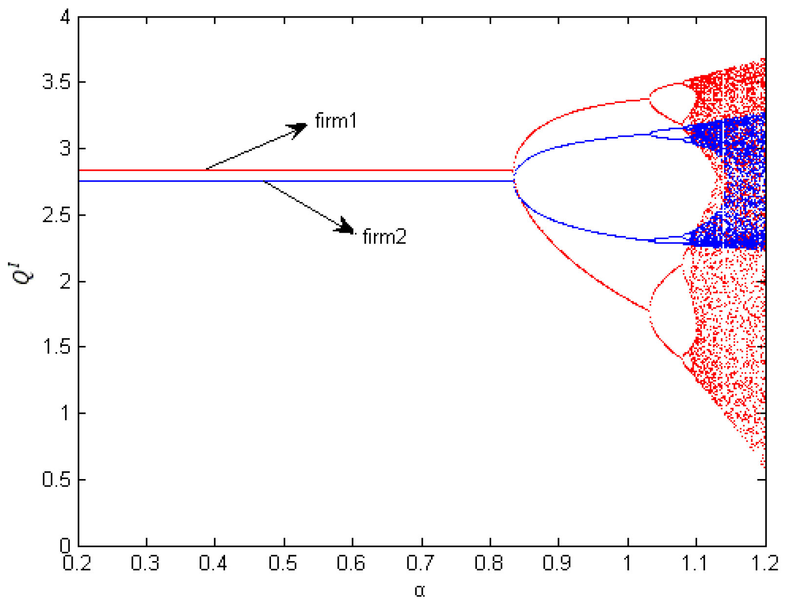
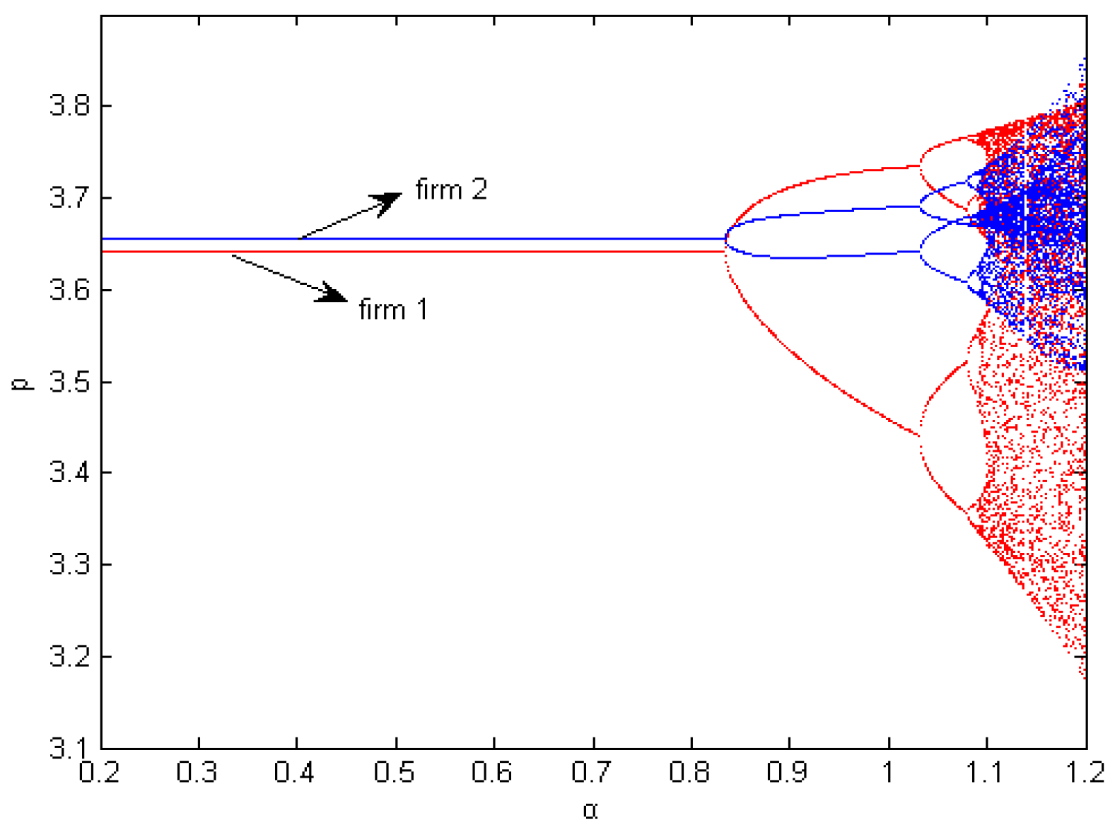
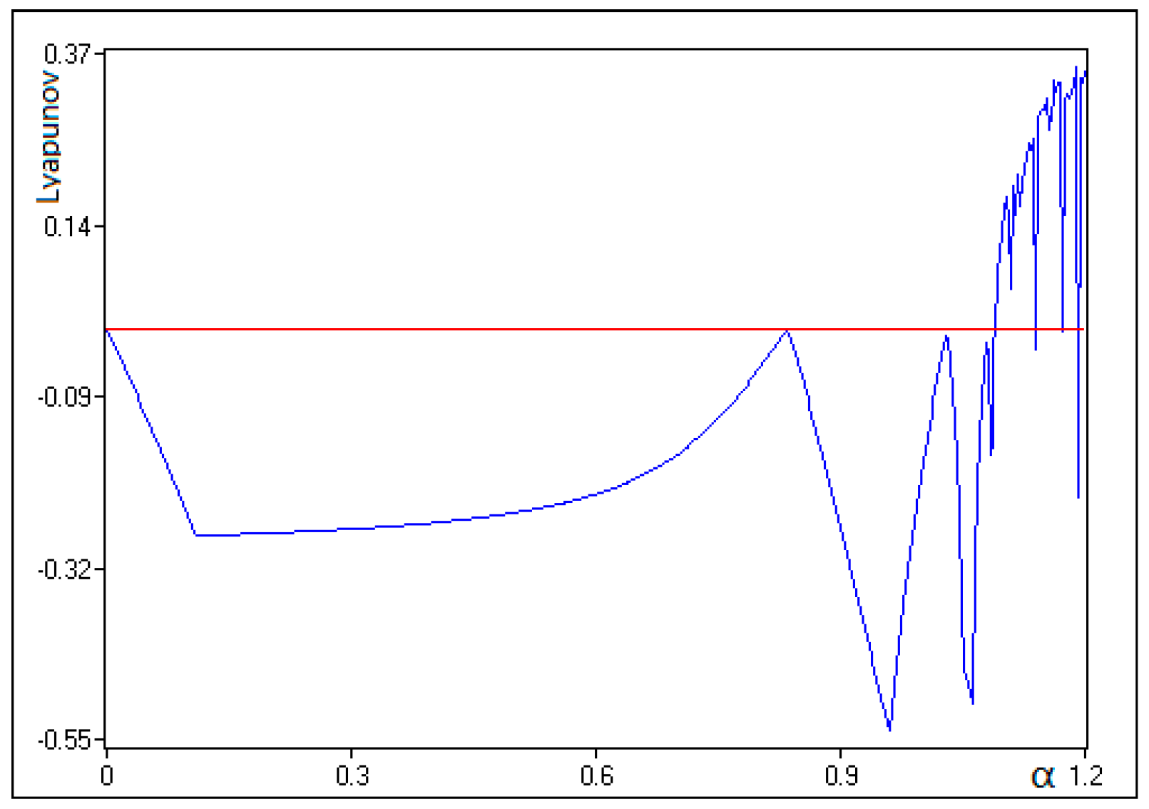
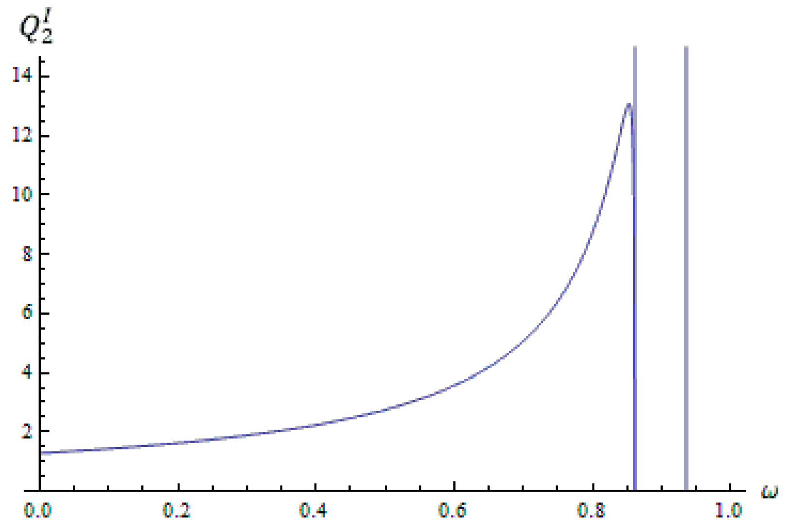
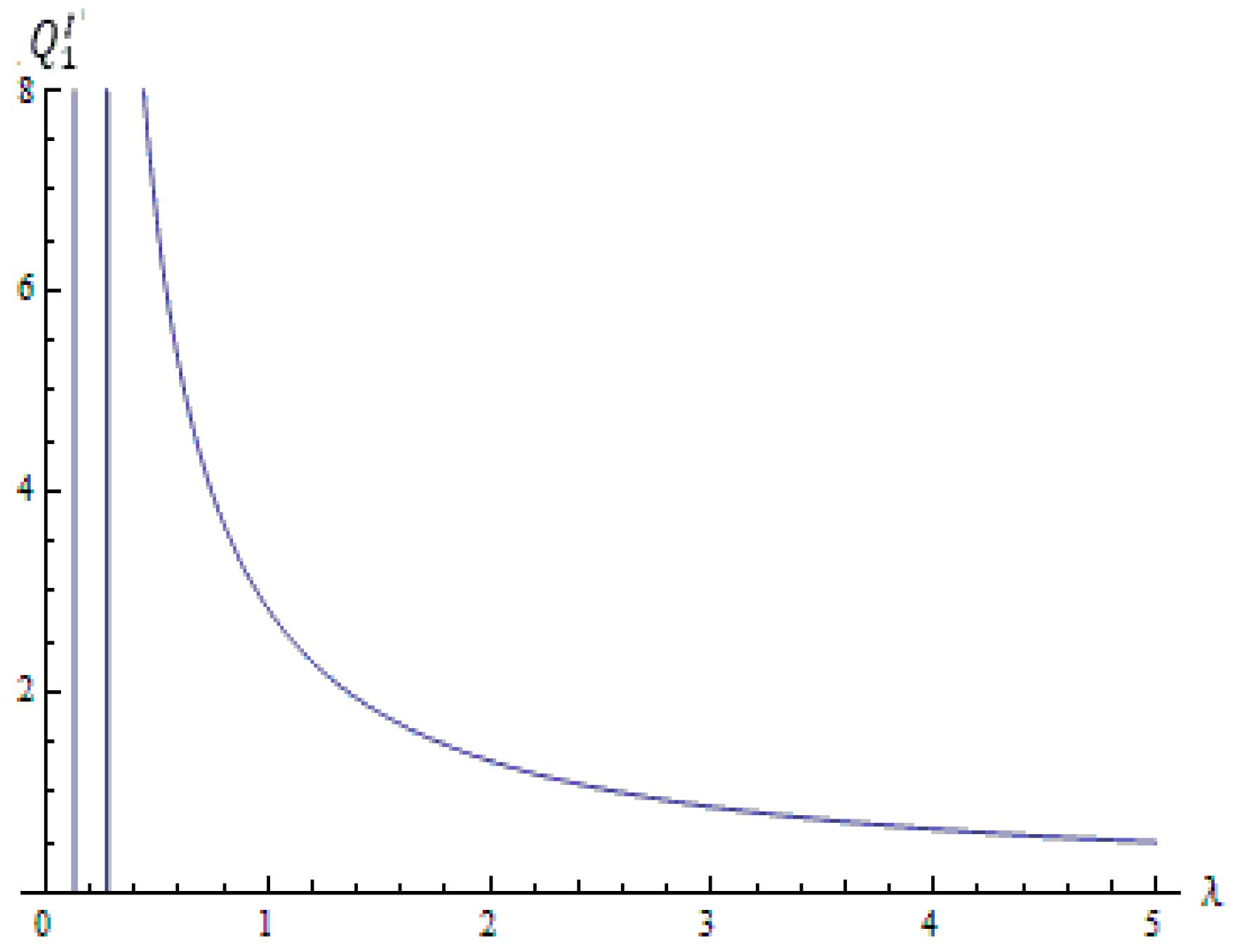
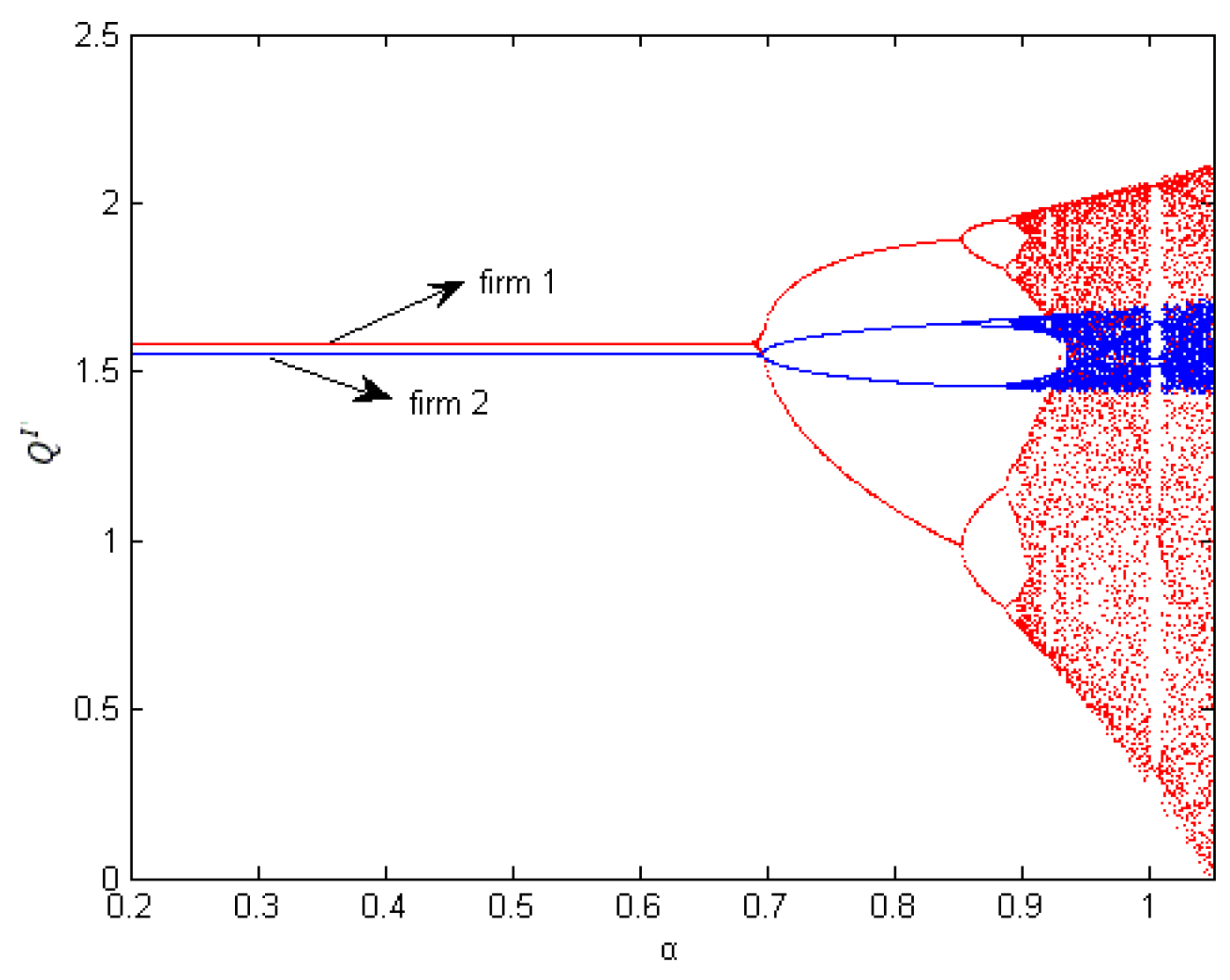
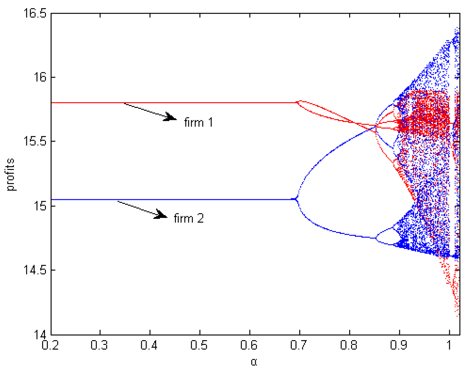
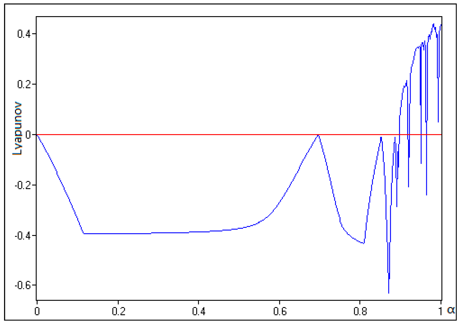
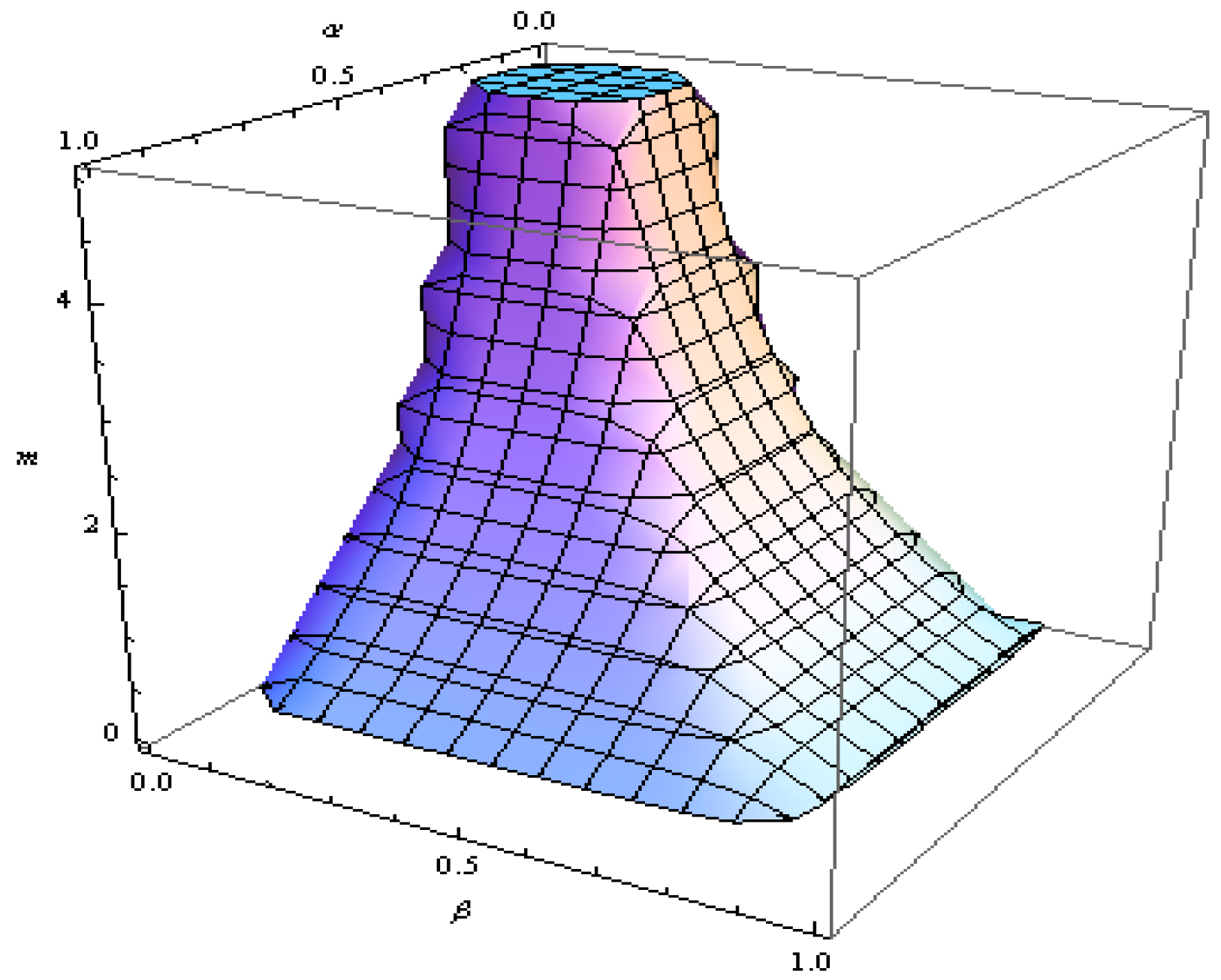
2.4.1. The Influence of the Decision Parameters on the Stability and the Entropy of the System

In order to study the impact of adjustment parameters on the system evolution, we set $\beta =0.8$, and we can describe the dynamic behavior and entropy of the system with varying $\alpha$. Figure 1, Figure 2 and Figure 3 show two firms’ innovation outputs, product prices and the profits as $\alpha$ changes. We can find that when $\alpha$ takes a small value, the equilibrium point is stable, but with $\alpha$ increasing, bifurcation occurs in the system and then the system even falls into chaos.

Figure 1. The innovation output bifurcation with change of α.

Figure 2. The product price bifurcation with change of α.

Figure 3. The profit bifurcation with change of α.

We know that entropy measures the chaotic degree of the system, so it is not difficult to find that the entropy of the system is increasing with $\alpha$. The entropy of the system shows the probability of some particular information, and it will increase with the increasing of the uncertainty of the information. When the entropy is high, the information is so uncertain that we will need more information to make it clear.

We can find in Figure 1 that when $\alpha$ is less than 0.85, the two firms’ innovation output ${Q^I}^{*}$ is a certain value, so the entropy is low. With $\alpha$ increasing, the value of the innovation output ${Q^I}^{*}$ goes from one certain value to two values. Finally when $\alpha$ is greater than 1.08, it has multiple values. With the increase of the uncertainty of the system, the entropy is increasing, so we can come to the conclusion that a too large decision parameter will lead to a large entropy to the system, and so that the companies will have to get more information to make an optimal decision.

Figure 4 shows the maximal Lyapunov exponent with α varying from 0 to 1.2. The maximal Lyapunov exponent reflects the state of the system. When it is equal to zero, it corresponds to the critical point of bifurcation in the system, and when it is larger than zero, it means the system falls into chaos with increased entropy. We can find in Figure 4 that when $\alpha$ takes a small value, the equilibrium point is stable, but with $\alpha$ increasing to a certain degree, the system falls into chaos, so the conclusion is the same as above. $\beta$ has a similar impact on the system as α has, as we have analyzed before.

Figure 4. The maximal Lyapunov exponent with change of α.

Figure 5 presents the parameter basin plots of the system with respect to parameters $\left(\alpha ,\beta \right)$, we use different colors to describe different states of the system, and that is, the stable state(red), cycles of periods 2 (yellow), 4 (green), 8 (pink), chaos (white) and divergence (black).

Figure 5. The parameter basin of the system.

Figure 6 shows the system’s sensitivity to the initial value. We set $\alpha =1.2,\beta =1.0$, in this condition the system falls into chaos. The firms’ initial innovation inputs are respectively taken as $Q_1^I=2.83,Q_2^I=2.75$ and ${Q_1^I}^{\text{'}}=2.831,{Q_2^I}^{\text{'}}=2.75$, then we get variation of the innovation output decisions from period 0 to 100. We can find that the system shows a significant difference after about 10 cycles of iteration, so when the system is in the state of chaos with high entropy, even a minor change in the initial value will cause a huge difference in later decisions.

Figure 6. The sensitivity to initial values of the system. (a) Comparison of the evolutions of the system taking two different initial values; (b) $\Delta Q_1^I$ in the period of 0–100 taking two different initial values.

By analyzing the influence of the decision parameters on the stability of the system, we can conclude that the firms should not take an overlarge adjustment parameter when making innovation output decisions, otherwise the system will fall into an unstable state with high entropy and have an adverse impact on the firms’ correctly making decisions and their profits.

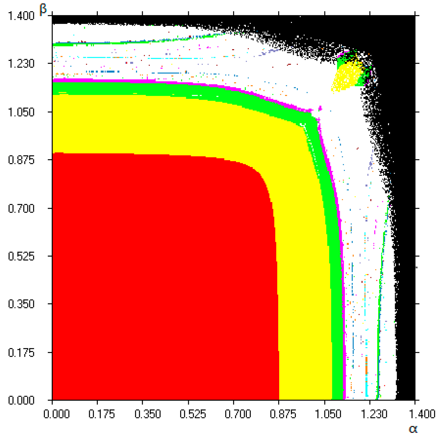
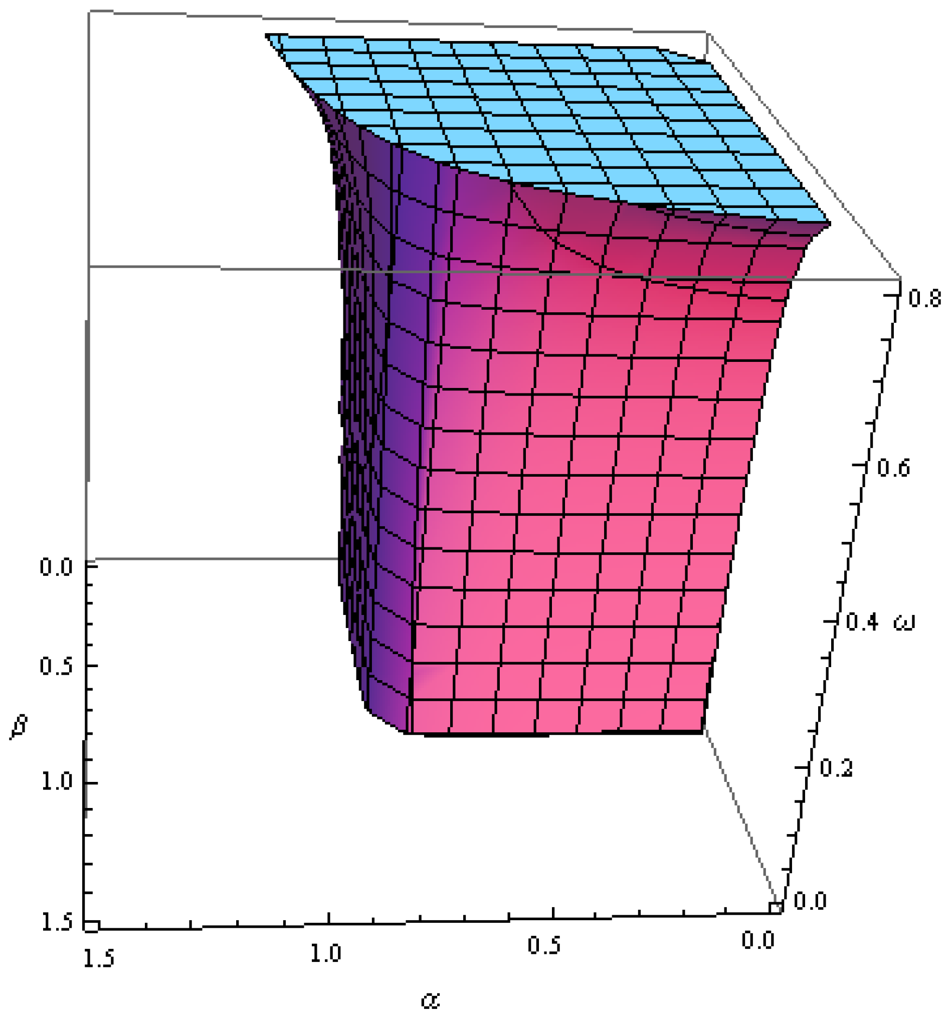
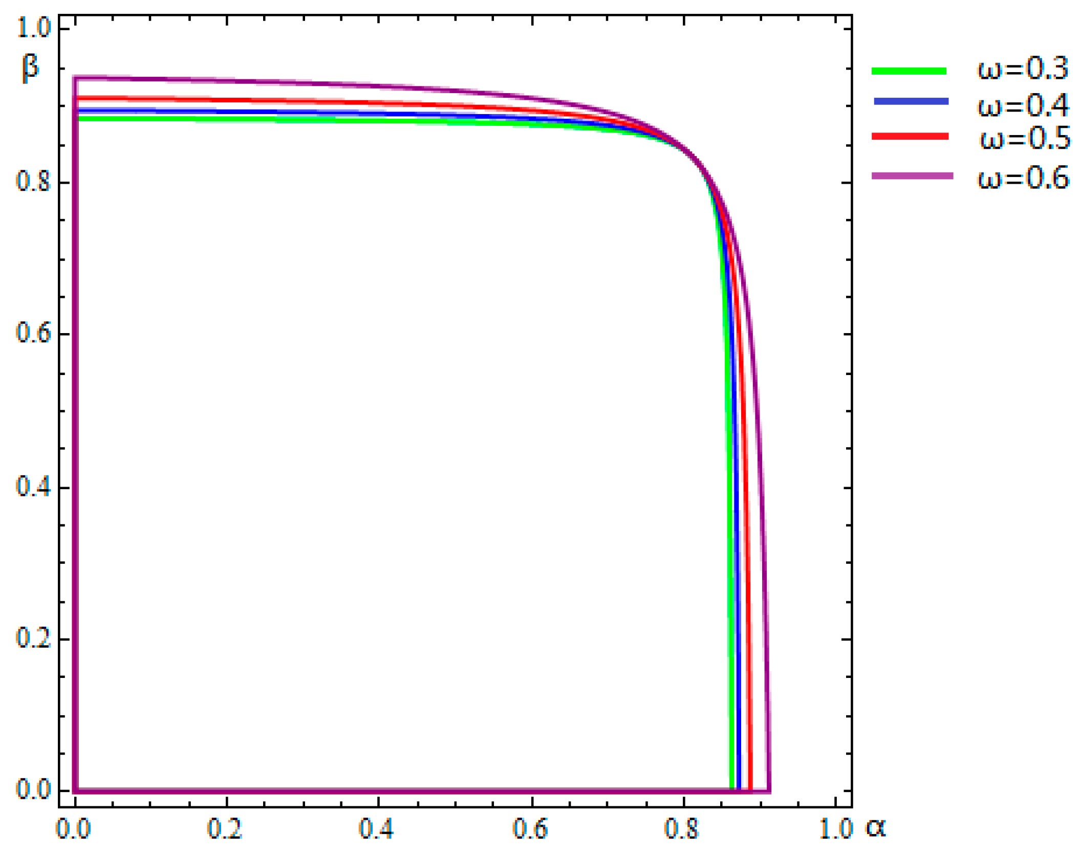
2.4.2. The Influence of Government Innovation Subsidy Rate on the Stability Region

We further set $a=8,b=2,c_1=0.5,c_2=0.6,\theta =0.6,\lambda =1$ and get the 3-D stability region of the system with change of $\alpha ,\beta ,\mathsf{\omega }$ in Figure 7 according to Jury stability criterion which is given in Equation (13). We can find that, as the government innovation subsidy rate $\omega$ increases, the stability region increases in the area of the $\alpha -\beta$ plane. So it can be concluded that an appropriate increase in the government subsidy rate of innovation can improve the stability of the system and decrease entropy. By drawing the stability region about $\alpha ,\beta$ with different government subsidy rates (Figure 8), we can draw the conclusion more clearly.

Figure 7. The 3-D stability region of the system with change of $\alpha ,\beta ,\omega$.

Figure 8. The stability regions of the system with changes in $\alpha , \beta$ (set different values of $\omega$).

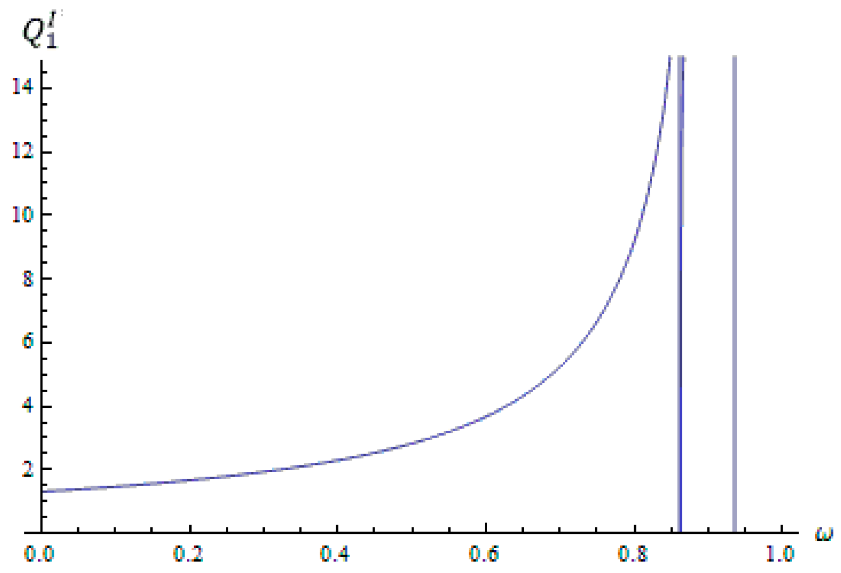
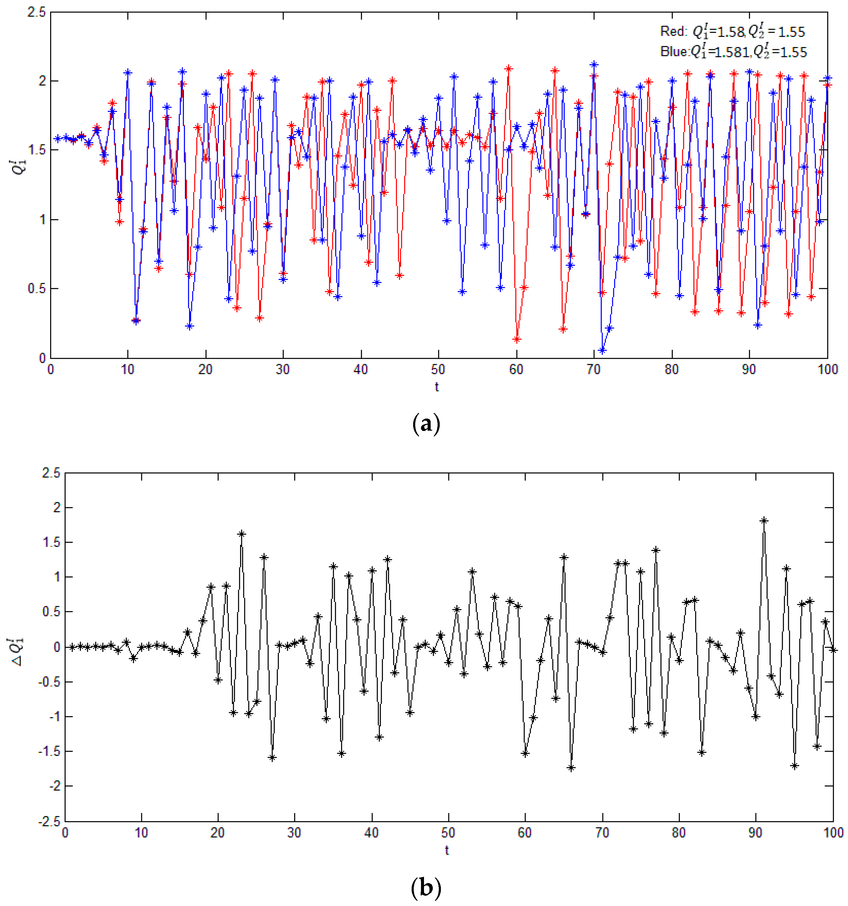
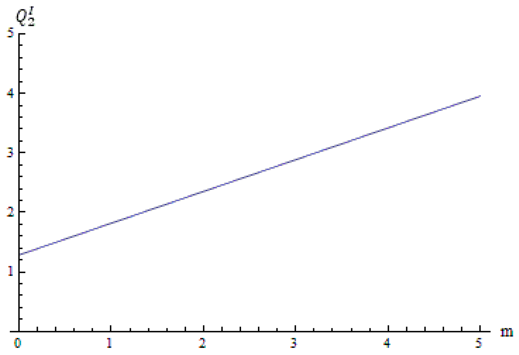
2.4.3. The Effect of the Government Innovation Subsidy Rate on Firms’ Innovation Activities

We also set $a=8;b=2;c_1=0.5;c_2=0.6;\theta =0.6;\lambda =1$, then we can get the equilibrium solution ${Q^I}^{*}=\left({Q_1^I}^{*},{Q_2^I}^{*}\right)$

$$\{\begin{array}{c}{Q_1^I}^{*}=\frac{1.06-1.23\omega }{0.81-1.80\omega +{\omega }^2}\\ {Q_2^I}^{*}=\frac{1.03-1.20\omega }{0.81-1.80\omega +{\omega }^2}\end{array}$$

(14)

Figure 9 and Figure 10 show how two firms’ innovation outputs vary with the changes in government innovation subsidy. We can conclude that the innovation outputs $Q_i^I$ increase along with the increase in the subsidy rate, and there’s a trend of increasing marginal. It indicates that the policy of government subsidies based on the innovation inputs plays a positive role in encouraging firms’ innovation activities, but we can see that when the subsidy rate is close to 1, the equilibrium solution is either too large or too small. In this condition the government pays almost all of the innovation activity funds, so firms may increase their innovation input infinitely, which will place too much fiscal burden to the government, so we should avoid the occurrence of this phenomenon in practice. Therefore, the government should synthetically determine a reasonable rate of subsidy to encourage firms’ innovation activities.

Figure 9. The relationship of $Q_1^I$ and $\omega .$

Figure 10. The relationship of $Q_2^I$ and $\omega$.

We have proved that the government’s innovation subsidy policies based on the innovation input had a positive effect on firms’ innovation activities, and the government should decide a reasonable subsidy rate $\omega$. Then we will analyze the optimal subsidy decision that the government should make.

The government’s goal is to maximaze the social welfare $W$, and the social welfare is the sum of the consumer surplus $CS$ and the producer surplus. According to the study of Lopez and Naylor [24], the consumer surplus $CS$ is defined as:

$$CS=U-p_1{Q}_1-p_2{Q}_2$$

(15)

in which $U$ is the consumer’s utility function.

We assume that consumer’s utility function $U$ has a quadratic relationship with the production [25], which means:

$$U=Q_1+Q_2-\frac{1}{2}\left({Q_1}^2+2\theta Q_1{Q}_2+{Q_2}^2\right)$$

(16)

Then we can get that the social welfare $W$ is:

$$W=CS+\left({\pi }_1+{\pi }_2\right)$$

(17)

Putting Equations (15) and (16) into (17), then we can get:

$$W=Q_1+Q_2-\frac{1}{2}\left({Q_1}^2+2\theta Q_1{Q}_2+{Q_2}^2\right)-p_1{Q}_1-p_2{Q}_2+\left({\pi }_1+{\pi }_2\right)$$

(18)

As we have analyzed above, we obtain ${p_1}^{*}$, ${p_2}^{*}$, ${Q_1^I}^{*},{Q_2^I}^{*}$, and putting them into Equation (3), then:

$$\{\begin{array}{c}{Q_1}^{*}=a-b\left({p_1}^{*}-\theta {p_2}^{*}\right)+ {Q_1^I}^{*}-\theta {Q_2^I}^{*}\\ {Q_2}^{*}=a-b\left({p_2}^{*}-\theta {p_1}^{*}\right)+ {Q_2^I}^{*}-\theta {Q_1^I}^{*}\end{array}$$

(19)

Putting Equations (4) and (19) into (18), we can get:

$$W={Q_1}^{*}+{Q_2}^{*}-\frac{1}{2}\left({Q_1}^{*2}+2\theta {Q_1}^{*}{Q_2}^{*}+{Q_2}^{*2}\right)-{p_1}^{*}{Q_1}^{*}-{p_1}^{*}{Q_2}^{*}+\left({{\pi }_1}^{*}+{{\pi }_2}^{*}\right)$$

(20)

Setting the same parameters as above, we have $a=8;b=2;c_1=0.5;c_2=0.6;\theta =0.6;\lambda =1$, then we can get:

$$W=\frac{-68.054+291.693\omega -467.735{\omega }^2+332.545{\omega }^3-88.45{\omega }^4}{{\left(0.806-1.797\omega +{\omega }^2\right)}^2}$$

(21)

In order to get the optimal subsidy rate $\omega$ that maximizes $W$, we let:

$$\frac{dW}{d\omega }=0\text{ and }\frac{d^{2}W}{d{\omega }^2}<0$$

(22)

Consider that $\omega$ ranges from 0 to 1, then we get ${\omega }^{*}=0.86$, so the government’s optimal subsidy rate $\omega$ is 0.86, which can bring the best benefits to society.

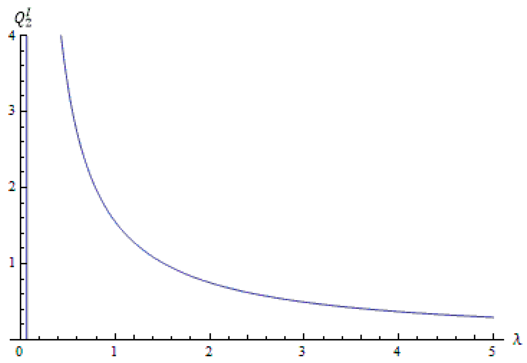
2.4.4. The Effect of the Innovation Input Parameter on Firms’ Innovation Activities

With the same parameters ($a=8;b=2;c_1=0.5;c_2=0.6;\theta =0.6;\omega =0.5$), we can get the equilibrium solution ${Q^I}^{*}=\left({Q_1^I}^{*},{Q_2^I}^{*}\right):$

$$\{\begin{array}{c}{Q_1^I}^{*}=\frac{2.46\lambda -0.68}{0.04-0.41\lambda +{\lambda }^2}\\ {Q_2^I}^{*}=\frac{2.41\lambda -0.68}{0.04-0.41\lambda +{\lambda }^2}\end{array}$$

(23)

Figure 11 and Figure 12 show how two firms’ innovation outputs vary with the innovation input parameter. We can find the innovation outputs $Q_i^I$ decrease along with the increase of parameter $\lambda$. We know that $\lambda$ measures the benefits brought by innovation acticities, and the smaller $\lambda$ is, the more benefits firms will obtain from the same capital spent on innovation. Therefore, firms are more willing to engage in innovation when $\lambda$ is smaller, so we advise that countries should support the cultivation of innovative talents and firms can improve their innovation ability by introducing talent, which will improve the earning of innovation and the innovation level of the whole society.

Figure 11. The relationship of $Q_1^I$ and $\lambda$.

Figure 12. The relationship of $Q_2^I$ and $\lambda .$

3. Government Financial Subsidies Based on Enterprises’ Innovation Outputs

3.1. The Model

In this section, we assume that the innovation subsidies given by the government are not based on the innovation inputs but on the innovation outputs, which means that government financial subsidies will be greater when there is higher innovation outputs of firms.

The elements in this model are the same as the last section except that the government’s innovation subsidy is $m(Q_i^I\left(t\right))$, in which m is the subsidy coefficient of innovation outputs, which represents the subsidies given for each increase of the market demand $Q^I$. So we can get the profit function of the two firms as:

$$\{\begin{array}{c}{\pi }_1\left(t\right)=\left(p_1\left(t\right)-c_1\right)\left(a-b\left(p_1\left(t\right)-\theta p_2\left(t\right)\right)+ Q_1^I\left(t\right)-\theta Q_2^I\left(t\right)\right)-\lambda {(Q_1^I\left(t\right))}^2+m(Q_1^I\left(t\right))\\ {\pi }_2\left(t\right)=\left(p_2\left(t\right)-c_2\right)\left(a-b\left(p_2\left(t\right)-\theta p_1\left(t\right)\right)+ Q_2^I\left(t\right)-\theta Q_1^I\left(t\right)\right)-\lambda \left(Q_2^I\left(t\right){)}^2+m(Q_2^I\left(t\right)\right)\end{array}$$

(24)

3.2. Model Solving

Same as illustrated above, we get two firms’ product prices in period t by maximizing their profits, then we get the equilibrium price as:

$$\{\begin{array}{c}{p}_1{\left(t\right)}^{*}=\frac{2a+2b{c}_1+a\theta +b{c}_2\theta +2Q_1^I\left(t\right)-{\theta }^2{Q}_1^I\left(t\right)-\theta Q_2^I\left(t\right)}{b\left(4-{\theta }^2\right)}\\ p_2{\left(t\right)}^{*}=\frac{2a+2b{c}_2+a\theta +b{c}_1\theta +2Q_2^I\left(t\right)-{\theta }^2{Q}_2^I\left(t\right)-\theta Q_1^I\left(t\right)}{b\left(4-{\theta }^2\right)}\end{array}$$

(25)

Putting (25) into (24), we get:

$$\{\begin{array}{c}{\mathsf{\pi }}_1\left(\mathrm{t}\right)=\left(p_1{\left(t\right)}^{*}-c_1\right)\left(a-b\left(p_1{\left(t\right)}^{*}-\theta p_2\left(t\right)\right)+Q_1^I\left(t\right)-\theta Q_2^I\left(t\right)\right)-\lambda {(Q_1^I\left(t\right))}^2+\mathrm{m}(Q_1^I\left(t\right))\\ {\mathsf{\pi }}_2\left(\mathrm{t}\right)=\left(p_2{\left(t\right)}^{*}-c_2\right)\left(a-b\left(p_2{\left(t\right)}^{*}-\theta p_1\left(t\right)\right)+Q_2^I\left(t\right)-\theta Q_1^I\left(t\right)\right)-\lambda {(Q_2^I\left(t\right))}^2+\mathrm{m}(Q_2^I\left(t\right))\end{array}$$

(26)

In the stage of innovation output decision, the firms make decisions based on the marginal profits, then:

$$\{\begin{array}{c}{Q}_1^I\left(t+1\right)=Q_1^I\left(t\right)+\alpha Q_1^I\left(t\right)\frac{\partial {\pi }_1\left(Q_1^I,Q_2^I\right)}{\partial Q_1^I\left(t\right)}\\ Q_2^I\left(t+1\right)=Q_2^I\left(t\right)+\beta Q_2^I\left(t\right)\frac{\partial {\pi }_2\left(Q_1^I,Q_2^I\right)}{\partial Q_2^I\left(t\right)}\end{array}$$

(27)

3.3. Analysis of the Equilibrium Point and the Stability of the System

Let $Q_i^I\left(t+1\right)=Q_i^I\left(t\right)$, we have assumed that both firms carry out innovation activities, so exclude $Q_i^I\left(t\right)=0$, then the unique equilibrium point of the system is:

$${Q^I}^{*}=\left({Q_1^I}^{*},{Q_2^I}^{*}\right)$$

(28)

In which

• ${Q_1^I}^{*}=(-2a\left(-2+{\theta }^2\right)\left(2-8b\lambda +\theta \left(2-4b\lambda \right)+{\theta }^3\left(-1+b\lambda \right)+{\theta }^2\left(-1+2b\lambda \right)\right)+b(-2c_1{\left(-2+{\theta }^2\right)}^2(1-4b\lambda +{\theta }^2\left(-1+b\lambda \right))+\left(-4+{\theta }^2\right)(-2b{c}_2\theta \left(-2+{\theta }^2\right)\lambda +m(-4-2\theta +{\theta }^3+16b\lambda +{\theta }^2(4-8b\lambda )+{\theta }^4\left(-1+b\lambda \right)))))/(2(-4{\left(1-4b\lambda \right)}^2+{\theta }^6{\left(-1+b\lambda \right)}^2+{\theta }^4\left(-5+16b\lambda -12b^2{\lambda }^2\right)+8{\theta }^2(1-5b\lambda +6b^2{\lambda }^2)))$
• ${Q_2^I}^{*}=(-2a\left(-2+{\theta }^2\right)\left(2-8b\lambda +\theta \left(2-4b\lambda \right)+{\theta }^3\left(-1+b\lambda \right)+{\theta }^2\left(-1+2b\lambda \right)\right)+b(-2c_2{\left(-2+{\theta }^2\right)}^2(1-4b\lambda +{\theta }^2\left(-1+b\lambda \right))+\left(-4+{\theta }^2\right)(-2b{c}_1\theta \left(-2+{\theta }^2\right)\lambda +m(-4-2\theta +{\theta }^3+16b\lambda +{\theta }^2(4-8b\lambda )+{\theta }^4\left(-1+b \lambda \right)))))/(2(-4{\left(1-4b\lambda \right)}^2+{\theta }^6{\left(-1+b\lambda \right)}^2+{\theta }^4\left(-5+16b\lambda -12b^2{\lambda }^2\right)+8{\theta }^2(1-5b\lambda +6b^2{\lambda }^2)))$

We analyze the equilibrium point and the stability of system by numerical simulation similar to that of Section 2.4, and we will show the parameter basin according to the Jury stability criterion in the next section.

3.4. Numerical Simulation

We set $m=0.5$ and keep other parameters the same as Section 2.4, they are $a=8;b=2;c_1=0.5;c_2=0.6;\theta =0.6;\lambda =1$. Then we can get the equilibrium point ${Q^I}^{*}=\left(1.58, 1.55\right)$.

3.4.1. The Influence of the Decision Parameters on the Stability and the Entropy of the System

Setting $\beta =0.6$, we can describe how the dynamic behavior of the system varies with $\alpha$ in Figure 13, Figure 14 and Figure 15. It is similar with Section 2.4, in that as $\alpha$ is increasing, bifurcation occurs in the system and then the system even falls into chaos.

Figure 13. The innovation output bifurcation with change of α.

Figure 14. The product price bifurcation with change of α.

Figure 15. The profit bifurcation with change of α.

We can also find that the entropy of the system is as $\alpha$ is increasing. We can find in Figure 13 that when $\alpha$ is less than 0.69, the two firms’ innovation output ${Q^I}^{*}$ has a certain value, so the entropy is low. Then with $\alpha$ increasing, the value of the innovation output ${Q^I}^{*}$ goes from one certain value to two values. Finally when $\alpha$ is greater than 0.89, it has multiple values.

The increase of uncertainty of the innovation output ${Q^I}^{*}$ will lead to the increase of the entropy of the system. Then we can come to the conclusion that a too large decision parameter will lead to a large entropy to the system, so companies will have to get more information to make an optimal decision.

Figure 16 shows the maximal Lyapunov exponent with α varying from 0 to 1.0. It can also reflect the transformation of the system from stability to bifurcation, then to chaos. The entropy of the system also increases in this process.

Figure 16. The maximal Lyapunov exponent with change of α.

Figure 17 shows the parameter basin plots of the system with respect to parameters $\left(\alpha ,\beta \right)$, where we can find that the system is stable when the decision parameters $\left(\alpha ,\beta \right)$ both take small values. We use different colors to describe different states of the system, and that is, the stable state (red), cycles of periods 2 (yellow), 4 (green), 8 (pink), chaos (white) and divergence (black).

Figure 17. The parameter basin of the system.

Figure 18 shows the system’s sensitivity to the initial value. We set $\alpha =1.0, \beta =0.9$, in this condition the system falls into chaos. The firms’ initial innovation inputs are respectively taken as $Q_1^I=1.58,Q_2^I=1.55$ and ${Q_1^I}^{\text{'}}=1.581,{Q_2^I}^{\text{'}}=1.55$, then we get variation of the innovation output decisions from period 0 to 100. We can find that the system shows a significant difference after about 18 cycles of iteration, so when the system is in the state of chaos with high entropy, even a minor change in the initial value will make a huge difference to later decisions.

Figure 18. The sensitivity to initial values of the system. (a) Comparison of the evolutions of the system taking two different initial values; (b) $\Delta Q_1^I$ in the period of 0–100 taking two different initial values.

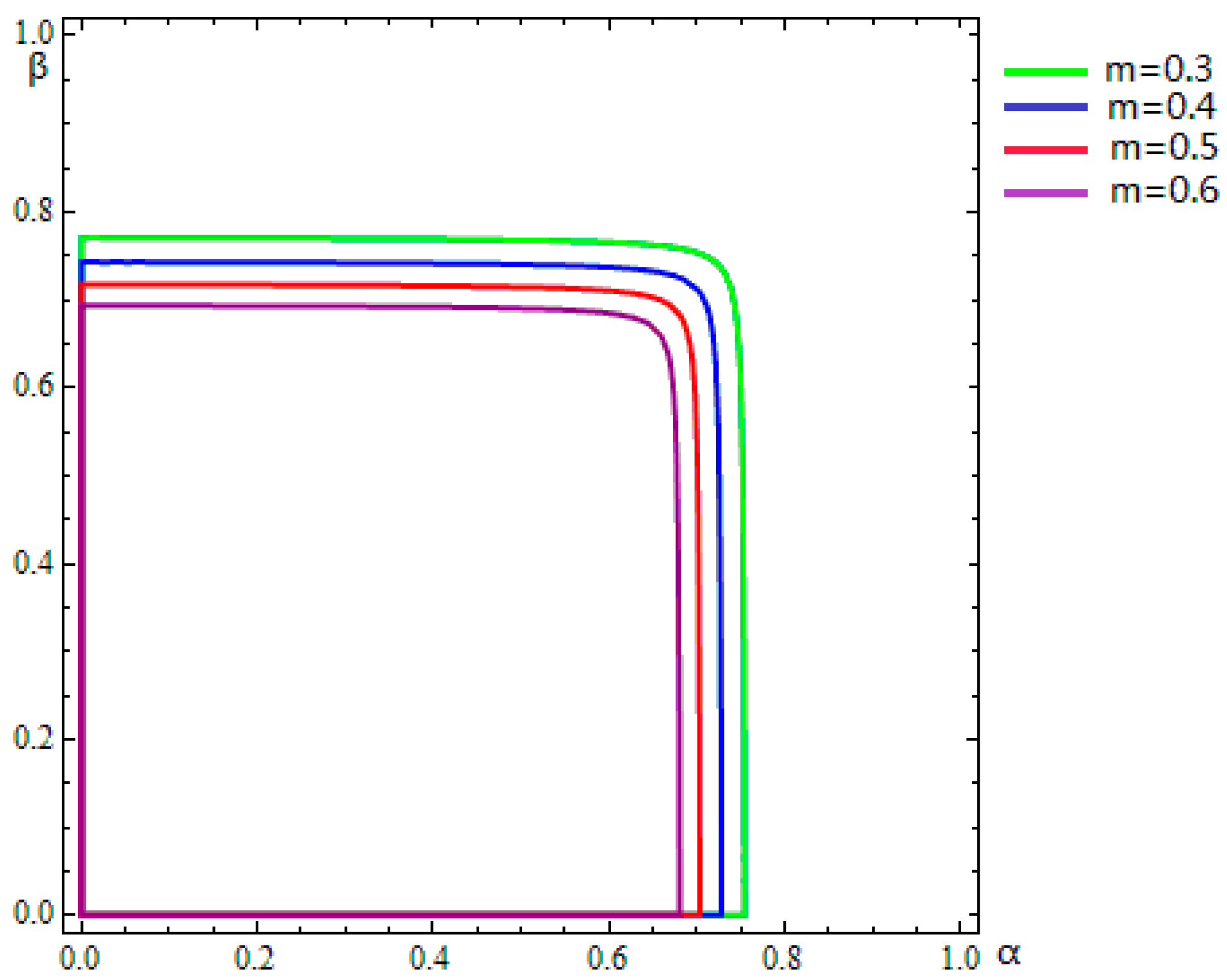
3.4.2. The Influence of the Subsidy Coefficient of Innovation Outputs to the Stability Region

We further set $a=8;b=2;c_1=0.5;c_2=0.6;\theta =0.6;\lambda =1$ and get the 3-D stability region of the system with change of $\left(\alpha ,\beta ,m\right)$ in Figure 19 according to the Jury stability criterion. We can find that as the subsidy coefficient of innovation outputs $m$ increases, the stability region decreases in the area of the $\alpha -\beta$ plane, so it can be concluded that the stability region can be affected by the value of $m$, but what is different from the last section is that the increase of the government’s subsidy coefficient will weaken the stability of the system and increase the entropy.

Figure 19. The 3-D stability region of the system with change of $\alpha ,\beta ,m$.

We can also draw the conclusion more clearly by drawing the stability region about $\alpha ,\beta$ with different government subsidy coefficients (Figure 20).

Figure 20. The stability regions of the system with changes in $\alpha ,\beta$ (set different values of $m$).

3.4.3. The Effect of the Subsidy Coefficient of Innovation Outputs on Firms’ Innovation Activities

With the parameter above ($a=8;b=2;c_1=0.5;c_2=0.6;\theta =0.6;\lambda =1$), we can get the equilibrium solution ${Q^I}^{*}=\left({Q_1^I}^{*},{Q_2^I}^{*}\right)$:

$$\{\begin{array}{c}{Q_1^I}^{*}=1.316+0.534m\\ {Q_2^I}^{*}=1.284+0.534m\end{array}$$

(29)

We can draw the conclusion from the expression of the equilibrium point and Figure 21 and Figure 22 that firms’ decisions on innovation outputs are proportional to the subsidy coefficient, which indicates that the policy of government subsidies based on the innovation outputs also plays a positive role in encouraging firms’ innovation activities, so governments should determine an appropriate subsidy coefficient $m$ by comprehensively considering the cost and price of the product and the effect on social welfare.

Figure 21. The relationship of $Q_1^I$ and $m$.

Figure 22. The relationship of $Q_2^I$ and $m$.

3.4.4. The Effect of the Innovation Input Parameter on Firms’ Innovation Activities

Set $a=8;b=2;c_1=0.5;c_2=0.6;\theta =0.6;m=0.5$, we get the equilibrium solution ${Q^I}^{*}=\left({Q_1^I}^{*},{Q_2^I}^{*}\right)$

$$\{\begin{array}{c}{Q_1^I}^{*}=\frac{1.48\lambda -0.20}{0.0089-0.2030\lambda +{\lambda }^2}\\ {Q_2^I}^{*}=\frac{1.45\lambda -0.20}{0.0089-0.2030\lambda +{\lambda }^2}\end{array}$$

(30)

We can draw the same conclusion from Figure 23 and Figure 24 that the innovation output $Q_i^I$ decreases with the increasing of parameter $\lambda$.

Figure 23. The relationship of $Q_1^I$ and $\lambda$.

Figure 24. The relationship of $Q_2^I$ and $\lambda$.

We have proved that the government’s innovation subsidy policies based on the innovation output have a positive effect on firms’ innovation activities, and the government should determine an appropriate subsidy coefficient $m$. Just as the study in Section 2.4.3, we can get the optimal subsidy coefficient of innovation output $m$.

We also set $a=8;b=2;c_1=0.5;c_2=0.6;\theta =0.6;\lambda =1$ as above, then we can get that:

$$W=-104.78-5.68m+0.42m^2$$

(31)

Let $\frac{dW}{dm}=0$, then we get that $m=6.71$. When $0\le m<6.71$, $\frac{d^{2}W}{d{m}^2}<0$. When $m>6.71$, $\frac{d^{2}W}{d{m}^2}>0$, so when $0\le m<6.71$, we will get the biggest social utility when $m=0$, but in this condition, there is no promoting effect on enterprises’ innovation activities. When $m>6.71$, the increase of $m$ will not only promote enterprises’ innovation activities, but also improve the social welfare, so the government should set the subsidy coefficient $m$ larger than 6.71.

4. Comparison of the Effects of the Two Kinds of Subsidy Policies on Innovation

In Section 2 and Section 3, we have analyzed the stability and the equilibrium solution of the system under two kinds of government subsidies, one is based on the innovation inputs and the other is based on the innovation outputs. We can conclude that:

(1)

In the aspect of stimulating firms’ innovation activities, the two kinds of subsidy policies both play a positive role, so the government can encourage firms’ innovation activities by increasing the subsidy rate $\omega$ or increasing the subsidy coefficient of innovation outputs $m$. What is different is that under the first policy, the relationship of the innovation output decision and the subsidy rate has a marginal increasing character, while under the second policy, firms’ innovation outputs decision is proportional to the subsidy coefficient. This means that the first policy, which is based on the innovation inputs, has a more significant incentive effect on innovation activities than the second policy, which is based on the innovation outputs.

(2)

In the aspect of stability of the system, the system will bifurcate and even fall into chaos with increasing entropy when taking large decision parameters $\left(\alpha ,\beta \right)$ in both models. Besides, the subsidy rate $\mathsf{\omega }$ and subsidy coefficient $m$ can both affect the stability region of the system. What is different is that the increase of the subsidy rate $\mathsf{\omega }$ can enhance the stability of the system while the increase of the subsidy coefficient $m$ will weaken the stability of the system and increase entropy.

5. Conclusions

In this paper, we propose two different forms of government subsidies based on innovation input and innovation output, respectively, and we establish a dynamic game model between two bounded rational enterprises. In the process, we analyze the complexity of the model, and we discuss the effect of two different forms of government subsidies on stimulating the innovation activities. At the same time, we analyze how the innovation decision’s adjusting speed, the degree of government subsidies and the beneficial coefficient of innovation influence the equilibrium, entropy and stability of the system. We draw the following conclusions:

(1)

Both kinds of innovation subsidy policies proposed in this paper have positive effects on firms’ innovation activities. Therefore, the government can increase firms’ enthusiasm for innovation by giving an appropriate government subsidy, which is beneficial to build a good innovative economic environment.

(2)

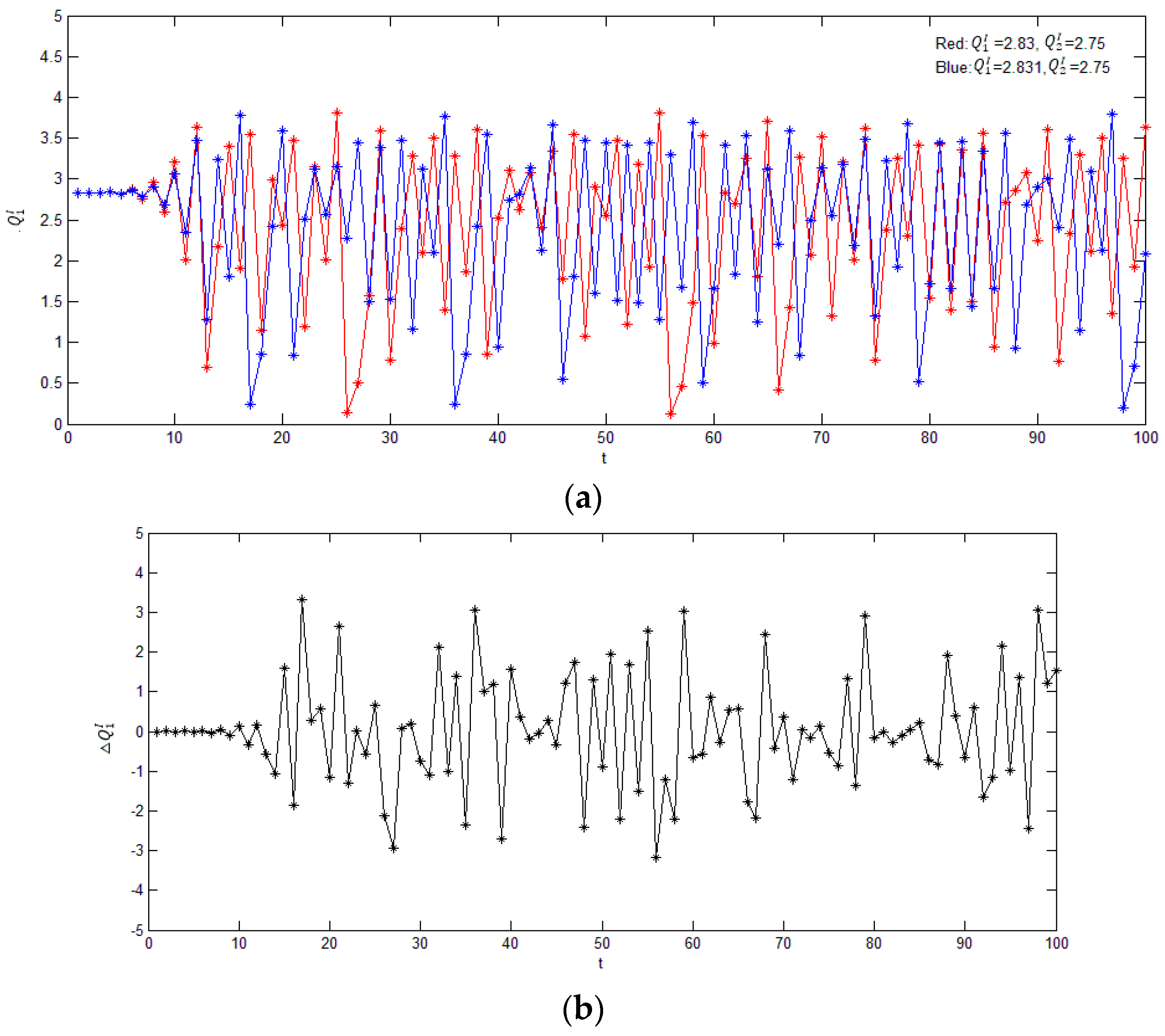
Assumed to be bounded rationally, the two firms make decisions of innovation outputs according to the marginal profit effect, but in the decision making process, the decision parameters $\alpha , \beta$ should not be too large, or the system will fall into the unstable state where decisions fluctuate disorderly and the entropy of the system will increase which means the companies will need more information to make an optimal decision.

(3)

The degree of the government innovation subsidies will impact the stability of the system. Under the subsidy policy based on the innovation inputs, the increase in subsidy rate $\omega$ can decrease the entropy and enhance the stability of the system, but under the subsidy policy based on the innovation outputs, the increase in the subsidy coefficient $m$ will increase the entropy and weaken the stability of the system, so the government should synthetically consider the effect of the innovation subsidy on innovation incentives, the stability of the system, the budget of fiscal expenditure and the social benefits, and then decide a rational subsidy rate $\omega$ or subsidy coefficient $m$.

(4)

The innovation input parameter $\lambda$ measures the benefits brought by innovation acticities, and the smaller is $\lambda$, the more benefits firms will obtain from the same investment in innovation, which means a higher level of inovation. The results derived from both models in this paper indicate that firms are more willing to engage in innovation when $\lambda$ is small, so we advise that countries should support the cultivation of innovative talents and firms can improve their innovation ability by introducing talents, which will improve the earning of innovation and the innovation level of the whole society.

There are two limitations in this paper that should be noticed, and these point to possible future research directions. Firstly, we followed the classic linear demand function when establishing the game model, but because of the randomness of the market, there may be some distinction between the real demands and the ideal demands, so in future research we will improve the demand function, for example, by adding a probability distribution function in the demand function to adapt to stochastic demand in the real market. Secondly, we assume that the players in the game are both bounded rationally. Either of them is the rival for the other, so neither of the two players can learn about the exact innovation output decision that its rival makes. This assumption is a good fit for a tit-for-tat game, but there are some other types of game where there exists information sharing between the players, which may bring a win-win result. We leave this for future research.

References

- González, X.; Pazó, C. Firms’ R&D dilemma: To undertake or not to undertake R&D. Appl. Econ. Lett. 2004, 11, 55–59. [Google Scholar]
- Hasnas, I.; Lambertini, L.; Palestini, A. Open Innovation in a dynamic Cournot duopoly. Econ. Model. 2014, 36, 79–87. [Google Scholar] [CrossRef]
- Toivanen, O.; Stoneman, P.; Bosworth, D. Innovation and the market value of UK firms. 1989–1995. Oxf. Bull. Econ. Stat. 2002, 64, 39–61. [Google Scholar] [CrossRef]
- Li, T.; Ma, J. The complex dynamics of R&D competition models of three oligarchs with heterogeneous players. Nonlinear Dyn. 2013, 74, 45–54. [Google Scholar]
- Fontana, R.; Nesta, L. Product innovation and survival in a high-tech industry. Rev. Ind. Organ. 2009, 34, 287–306. [Google Scholar] [CrossRef]
- Lambertini, L.; Mantovani, A. Process and product innovation: A differential game approach to product life cycle. Int. J. Econ. Theory 2010, 6, 227–252. [Google Scholar] [CrossRef]
- Park, S. Evaluating the efficiency and productivity change within government subsidy recipients of a national technology innovation research and development program. R&D Manag. 2015, 45, 549–568. [Google Scholar]
- Catozzella, A.; Vivarelli, M. Beyond Additionality: Are Innovation Subsidies Counterproductive; Social Science Electronic Publishing: Rochester, NY, USA, 2011. [Google Scholar]
- Huang, Q.; Jiang, M.S.; Miao, J. Effect of government subsidization on Chinese industrial firms’ technological innovation efficiency: A stochastic frontier analysis. J. Bus. Econ. Manag. 2016, 17, 187–200. [Google Scholar] [CrossRef]
- Fölster, S. Do subsidies to cooperative R&D actually stimulate R&D investment and cooperation? Res. Policy 1995, 24, 403–417. [Google Scholar]
- Un, C.A.; Montoro-Sanchez, A. Public funding for product, process and organisational innovation in service industries. Serv. Ind. J. 2010, 30, 133–147. [Google Scholar] [CrossRef]
- Kang, K.N.; Park, H. Influence of government R&D support and inter-firm collaborations on innovation in Korean biotechnology SMEs. Technovation 2012, 32, 68–78. [Google Scholar]
- Guo, D.; Guo, Y.; Jiang, K. Government-subsidized R&D and firm innovation: Evidence from China. Res. Policy 2016, 45, 1129–1144. [Google Scholar]
- Hinloopen, J. Subsidizing cooperative and noncooperative R&D in duopoly with spillovers. J. Econ. 1997, 66, 151–175. [Google Scholar]
- Hinloopen, J. More on subsidizing cooperative and noncooperative R&D in duopoly with spillovers. J. Econ. 2000, 72, 295–308. [Google Scholar]
- Kleer, R. Government R&D subsidies as a signal for private investors. Res. Policy 2010, 39, 1361–1374. [Google Scholar]
- Lerner, J. The government as venture capitalist: The long-run impact of the SBIR program. J. Priv. Equity 2000, 3, 55–78. [Google Scholar] [CrossRef]
- Meuleman, M.; de Maeseneire, W. Do R&D subsidies affect SMEs’ access to external financing? Res. Policy 2012, 41, 580–591. [Google Scholar]
- Takalo, T.; Tanayama, T. Adverse selection and financing of innovation: Is there a need for R&D subsidies? J. Technol. Transf. 2010, 35, 16–41. [Google Scholar]
- Zapart, C.A. On entropy, financial markets and minority games. Phys. A Stat. Mech. Appl. 2009, 388, 1157–1172. [Google Scholar] [CrossRef]
- Han, Z.; Ma, J.; Si, F.; Ren, W. Entropy complexity and stability of a nonlinear dynamic game model with two delays. Entropy 2016, 18, 317. [Google Scholar] [CrossRef]
- D’Aspremont, C.; Jacquemin, A. Cooperative and noncooperative R&D in duopoly with spillovers. Am. Econ. Rev. 1988, 78, 1133–1137. [Google Scholar]
- Bischi, G.I.; Lamantia, F. A competition game with knowledge accumulation and spillovers. Int. Game Theory Rev. 2004, 6, 323–341. [Google Scholar] [CrossRef]
- López, M.C.; Naylor, R.A. The Cournot–Bertrand profit differential: A reversal result in a differentiated duopoly with wage bargaining. Eur. Econ. Rev. 2004, 48, 681–696. [Google Scholar] [CrossRef]
- Symeonidis, G. Downstream merger and welfare in a bilateral oligopoly. Int. J. Ind. Organ. 2010, 28, 230–243. [Google Scholar] [CrossRef]
© 2016 by the authors; licensee MDPI, Basel, Switzerland. This article is an open access article distributed under the terms and conditions of the Creative Commons Attribution (CC-BY) license (http://creativecommons.org/licenses/by/4.0/).