Optimization of Two-Stage Peltier Modules: Structure and Exergetic Efficiency

Abstract

In this paper we undertake the theoretical analysis of a two-stage semiconductor thermoelectric module (TEM) which contains an arbitrary and different number of thermocouples, $n_1$ and $n_2$, in each stage (pyramid-styled TEM). The analysis is based on a dimensionless entropy balance set of equations. We study the effects of $n_1$ and $n_2$, the flowing electric currents through each stage, the applied temperatures and the thermoelectric properties of the semiconductor materials on the exergetic efficiency. Our main result implies that the electric currents flowing in each stage must necessarily be different with a ratio about 4.3 if the best thermal performance and the highest temperature difference possible between the cold and hot side of the device are pursued. This fact had not been pointed out before for pyramid-styled two stage TEM. The ratio $n_1/n_2$ should be about 8.

1. Introduction

Thermoelectric cooling systems (TEC) usually consist of a thermoelectric module (TEM) with one or more stages and heat exchangers at the cold side and the hot side of the module. These kind of devices are widely used to control the temperature of electronic components which have important applications in many fields such as thermoelectric refrigeration, aerospace applications, small instruments cooling, dehumidification, food conservation, etc. [1]. There are several factors affecting the performance of TECs, such as the properties of the semiconductor materials [2], the size of thermocouples, the junction temperature, the electrical current [3], etc. The methods used to study this problem include optimal control theory [4], nonequilibrium thermodynamics [5], finite time thermodynamics [6], among others. An interesting series of applications of two stage thermoelectric modules has been reported in [7,8,9,10,11,12,13]. The optimization of the devices yields an improved performance. Yamanashi [3] used heat balance equations to analyze the coefficient of performance (COP) of a thermoelectric cooler including heat exchangers at the cold and hot side of the device. The balance equations follow from non-equilibrium thermodynamics and a deduction can be seen in [14]. In [15] the optimization of two-stage thermoelectric coolers in two configurations was presented. Two arrangements were considered, the so-called pyramid-styled by the authors and the cuboid-styled coolers. The study was carried out by using the COP as the optimization criterion. In the case of the pyramid-styled cooler, it was found that the ratio of the number of thermocouples between the stages must be 2.5–3. The same conclusion was obtained for the ratio of the flowing electric currents in the stages for the cuboid-styled one but a similar study is lacking in the case of pyramid-styled coolers. In [2] the authors considered a two-stage thermoelectric cooler and studied the influence of the number of thermocouples and the area of each one and the electric current in the first stage on the performance of the system measured through the COP. The conclusion was that for a fixed current in the first stage, the increase of the area of every thermocouple and the decrease of the number of them in the stage improved the COP. In the present work an irreversible thermodynamic analysis is done about the performance of a two-stage TEM (no exchangers included) by using dimensionless entropy balance equations [3] when the thermoelectric properties of the p and n arms of thermocouples are independent of temperature. The performance depends not only on the mentioned physical properties, but also on the configuration of the cooler, i.e., the number of thermocouples in each stage, and the flowing electric current through each one. All the above mentioned aspects of the thermodynamics of TECs will be considered here focusing on the determination of the optimal configuration of the TEM measured by the exergetic efficiency. Special emphasis will be put on the influence of the configuration of the TEM and the ratio of working electric currents on the exergetic efficiency in the case of pyramid-styled TEMs. Multi-stage semiconductor thermoelectric modules are often used for extending operating difference temperature range of the semiconductor thermoelectric cooling by keeping a reasonable thermal efficiency. This has motivated the theoretical and experimental research on improving the performance of two-stage semiconductor thermoelectric coolers, which is why we choose the exergetic efficiency to measure the performance of the system.

Section 2 is devoted to obtain the dimensionless heat rate balance equations for a two-stage TEM which constitute the theoretical basis of our study. In Section 3 we examine the influence of the physical parameters on the exergetic efficiency $\left(\varphi \right).$ This section contains our main results on the optimization of the configuration of the TEM. We close the paper with Section 4 where some discussion and conclusions can be found.

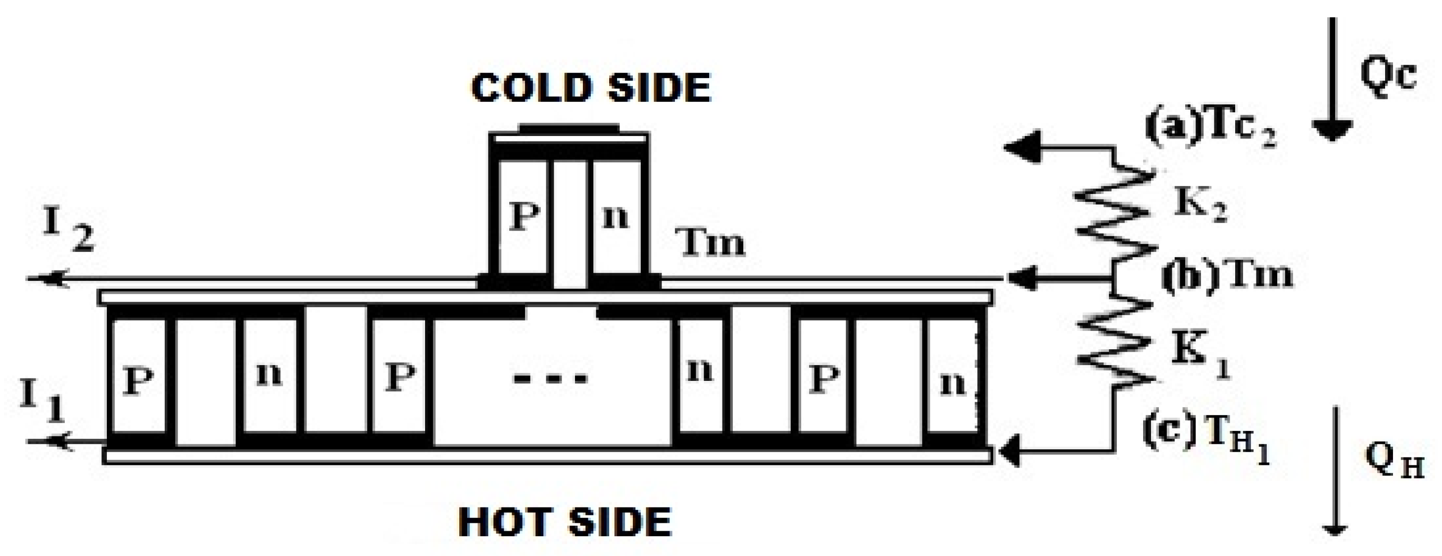
2. Heat Balance Equations

The TEM which is going to be analyzed here [2] consists of two stages denoted as 1 (which has $n_1$ thermocouples) and 2 with $n_2$ thermocouples (Figure 1). The thermocouples in each stage are electrically connected in series and thermally in parallel. The two stages are thermally connected in series. Each stage has its own working electric current I since a better performance can be achieved in this way as it will be shown in Section 4.

Figure 1. Schematic diagram of a thermoelectric cooler system with two stages.

The performance of a stage is determined by the electrical resistivity ρ, the Seebeck coefficient α, and the thermal conductivity κ of p and n arms. Though these three parameters depend in principle on the temperature, for the sake of simplicity it is assumed here that they have constant values. Before deriving the heat balance equations of the TEM system, the electrical resistance R, Seebeck coefficient A, and thermal conductance K of a stage must be given as follows [2]

$$R=n({\rho }_p+{\rho }_n)\frac{l}{S}$$

(1)

$$A=n({\alpha }_p+{\alpha }_n)$$

(2)

$$K=n({\kappa }_p+{\kappa }_n)\frac{S}{l}$$

(3)

where l is the length of p and n semiconductor arms, S is the cross-sectional area of p and n arms, n is the number of thermocouples in the stage, and subscripts p and n in Equations (1)–(3) designate p and n-type semiconductor, respectively. Unless otherwise noted, the parameters R, A and K have different values for each stage. Heat balance at each position from (a) to (c) in Figure 1 leads to [2]

$$Q_{C_2}=\left(A_2{I}_2{T}_{C_2}-\frac{1}{2}{I}_2^2{R}_2-K_2(T_m-T_{C_2})\right)n_2$$

(4)

$$Q_{H_2}=\left(A_2{I}_2{T}_{H_2}+\frac{1}{2}{I}_2^2{R}_2-K_2(T_m-T_{C_2})\right)n_2$$

(5)

$$Q_{C_1}=\left(A_1{I}_1{T}_{C_1}-\frac{1}{2}{I}_1^2{R}_1-K_1(T_{H_1}-T_m)\right)n_1$$

(6)

$$Q_{H_1}=\left(A_1{I}_1{T}_{H_1}+\frac{1}{2}{I}_1^2{R}_1-K_1(T_{H_1}-T_m)\right)n_1$$

(7)

where $Q_C$ is the heat rate that enters the thermoelectric module of each stage from the cold side and $Q_H$ the heat rate that goes out at the hot side. $T_C$ is the temperature of the cold side of the module, $T_H$ is the temperature of the hot side, $T_m$ is the contact temperature between the two stages of the TEM (note that $T_{H_2}=T_{C_1}=T_m)$ and I is the electrical current that flows through each one. The equations representing the total heat which enters the system and the final heat rate going out are Equations (4) and (7) where $n_2=N_T/(r+1)$ and $n_1=r{N}_T/(r+1)$, being $N_T$ the total number of thermocouples in the TEM, $N_T=$$n_1+n_2,$ and r the ratio $n_1/n_2.$ To make this paper self-contained and clarify their physical content, Equations (4) and (7) have been obtained in the Appendix at the end.

We now rewrite Equations (4) and (7) in dimensionless form in order to have a valid set of equations for any TEM. Following [3], we define the dimensionless variables

$$j_1=\frac{A_1{I}_1}{K_1},j_2=\frac{A_2{I}_2}{K_2}$$

(8)

$$q_{C_1}=\frac{Q_{C_1}}{N_T{K}_1{T}_{C_1}},q_{C_2}=\frac{Q_{C_2}}{N_T{K}_2{T}_{C_2}}$$

(9)

$$q_{H_1}=\frac{Q_{H_1}}{N_T{K}_1{T}_{H_1}},q_{H_2}=\frac{Q_{H_2}}{N_T{K}_2{T}_{H_2}}$$

(10)

$${\theta }_{H_1}=\frac{T_{H_1}}{T_m}$$

(11)

$${\theta }_{C_2}=\frac{T_{C_2}}{T_m}$$

(12)

$${\theta }_T=\frac{T_{H_1}}{T_{C_2}}=\frac{{\theta }_{H_1}}{{\theta }_{C_2}}$$

(13)

$$Z{T}_{C_2}=\frac{A_2^2{T}_{C_2}}{R_2{K}_2}$$

(14)

$$Z{T}_{m_1}=\frac{A_1^2{T}_m}{R_1{K}_1},Z{T}_{m_2}=\frac{A_2^2{T}_m}{R_2{K}_2}$$

(15)

$$Z{T}_{H_1}=\frac{A_1^2{T}_{H_1}}{R_1{K}_1}$$

(16)

In this way, $j_1$ and $j_2$ are dimensionless electric currents flowing through each stage of the TEM. $q_{C_2}$ and $q_{H_1}$ can be considered as the nondimensional entropy rate due to the presence of respective temperatures in the denominator of their definitions. Nevertheless, we will continue naming them as heat rates in the remaining of the paper. ${\theta }_T$ are the ratio of the hot side and cold side temperatures, respectively. $Z{T}_C$, $Z{T}_H$ and $Z{T}_m$ are dimensionless figures of merit associated with the temperatures $T_C$, $T_H$ and $T_m$, respectively. These temperatures would determine the values of the coefficients A, R and K in the case that they were dependent quantities on the temperature. Equations (4)–(7) can now be rewritten in terms of the dimensionless quantities defined by Equations (8)–(16). The result is

$$q_{C_2}=\left(j_2-{\theta }_{C_2}^{-1}+1-\frac{1}{2}{j}_2^2\frac{1}{Z{T}_{C_2}}\right)\frac{1}{r+1}$$

(17)

$$q_{H_2}=\left(j_2+{\theta }_{C_2}-1+\frac{1}{2}{j}_2^2\frac{1}{Z{T}_{m_2}}\right)\frac{1}{r+1}$$

(18)

$$q_{C_1}=\left(j_1-{\theta }_{H_1}+1-\frac{1}{2}{j}_1^2\frac{1}{Z{T}_{m_1}}\right)\frac{r}{r+1}$$

(19)

$$q_{H_1}=\left(j_1+{\theta }_{H_1}^{-1}-1+\frac{1}{2}{j}_1^2\frac{1}{Z{T}_{H_1}}\right)\frac{r}{r+1}$$

(20)

We mention that these equations also allow us to evaluate the effects of the thermoelectric properties of the material semiconductors represented by the figures of merit $Z{T}_C$, $Z{T}_H$ and $Z{T}_m$ on the performance of the TEM. Note that given the two electric currents $j_1$ and $j_2$, the contact temperature $T_m$ between the two stages of the TEM can be calculated from the condition $q_{H_2}=q_{C_1}$ in the following way

$$T_m=\frac{T_{C_2}+T_{H_1}r+\frac{1}{2}\left(R_1{K}_1{j}_1^{2}r/A_1^2+R_2{K}_2{j}_2^2/A_2^2\right)}{1-j_2+r(j_1+1)}$$

(21)

We define the dimensionless power p and the dimensionless voltage v as

$$p=\frac{Q_{H_1}-Q_{C_2}}{K_2{T}_{C_2}{N}_T}={\theta }_T{q}_{H_1}-q_{C_2}$$

(22)

and

$$v=\frac{p}{j}$$

(23)

Another expression of v is

$$v=\frac{V}{A{T}_{C_2}{N}_T}$$

(24)

where V is the voltage of the thermoelectric cooler.

3. Exergy Flow and Exergetic Efficiency

In this section we obtain the exergetic efficiency which will be used as the optimization variable. We begin by defining the exergy flow at the cold side of the TEM (a in Figure 1) as the work produced by the Carnot’s cycle between the temperatures $T_{H_1}$ and $T_{C_2}$. The flow of exergy is then given by

$$E_t=Q_{H_1}-Q_{C_2}$$

(25)

where $Q_{H_1}$ is the heat rate going from a reservoir at temperature $T_{H_1}$ to the Carnot’s cycle and $Q_{C_2}$ is the heat rate going from the Carnot’s cycle to environment at temperature $T_{C_2}$. Since in a Carnot’s cycle there is no entropy generation we have

$$\frac{Q_{H_1}}{T_{H_1}}-\frac{Q_{C_2}}{T_{C_2}}=0$$

(26)

Eliminating $Q_{H_1}$ in Equations (25) and (26), the exergy flow equation at the cold side is given by

$$E_t=(T_{H_1}-T_{C_2})\frac{Q_{C_2}}{T_{C_2}}$$

(27)

The exergetic efficiency [16] Φ of the TEM is defined as

$$\Phi =\frac{E_t}{P}$$

(28)

where P is the electrical power supplied to the system. Another expression for the efficiency reads

$$\varphi =\frac{{\epsilon }_t}{p}$$

(29)

being the dimensionless exergy flow ${\epsilon }_t$ defined as

$${\epsilon }_t=\frac{E_t}{N_T{K}_2{T}_{C_2}}=\left({\theta }_T-1\right)q_{C_2}$$

(30)

and p given by Equation (22).

We finally obtain the following expression for the exergetic efficiency ϕ by using Equation (17)

$$\varphi =\frac{({\theta }_T-1)(j_2-{\theta }_{C_2}^{-1}+1-\frac{1}{2}{j}_2^2\frac{1}{Z{T}_{C_2}})}{\Delta }$$

(31)

where

$$\begin{array}{cc}\hfill \Delta & ={\theta }_{T}r(j_1-1+{\theta }_{H_1}^{-1}+\frac{1}{2}{j}_1^2\frac{1}{Z{T}_{H_1}})-j_2+{\theta }_{C_2}^{-1}-1\hfill \\ & +\frac{1}{2}{j}_2^2\frac{1}{Z{T}_{C_2}}\hfill \end{array}$$

(32)

It has been discussed in the literature the usefulness of the exergetic efficiency given by Equation (31) to analyze the performance of thermoelectric devices. In order to clarify the reason why we adopt it as the performance criterion, it is first necessary to introduce the performance coefficient COP of the TEM, which is given by

$$COP=\frac{Q_{C_2}}{Q_{H_1}-Q_{C_2}}=\frac{q_{C_2}}{{\theta }_T{q}_{H_1}-q_{C_2}}$$

(33)

Substitution of Equations (13), (17) and (20) in Equation (33) yields:

$$COP=\frac{j_2-{\theta }_{C_2}^{-1}+1-\frac{1}{2}{j}_2^2\frac{1}{Z{T}_{C_2}}}{\Delta }$$

(34)

In this way, the efficiency Φ can be also considered as the ratio of the TEM’s COP ($Q_{C_2}/P,$ see Equation (33)) and that of the Carnot’s cycle ($Q_{C_2}/E_t$) [3]. It can be shown that the performance coefficient increases when the difference temperature $T_{H_1}-T_{C_1}$ decreases. This means that seeking a larger value of the COP implies a reduction in the TEM’s ability to generate temperature difference. The exergetic efficiency, on the other hand, has a maximum for certain values of $T_{H_1}$ and $T_{C_1}$. It represents a sort of compromise between a good performance and a significant temperature difference between the cold and the hot side of the system. 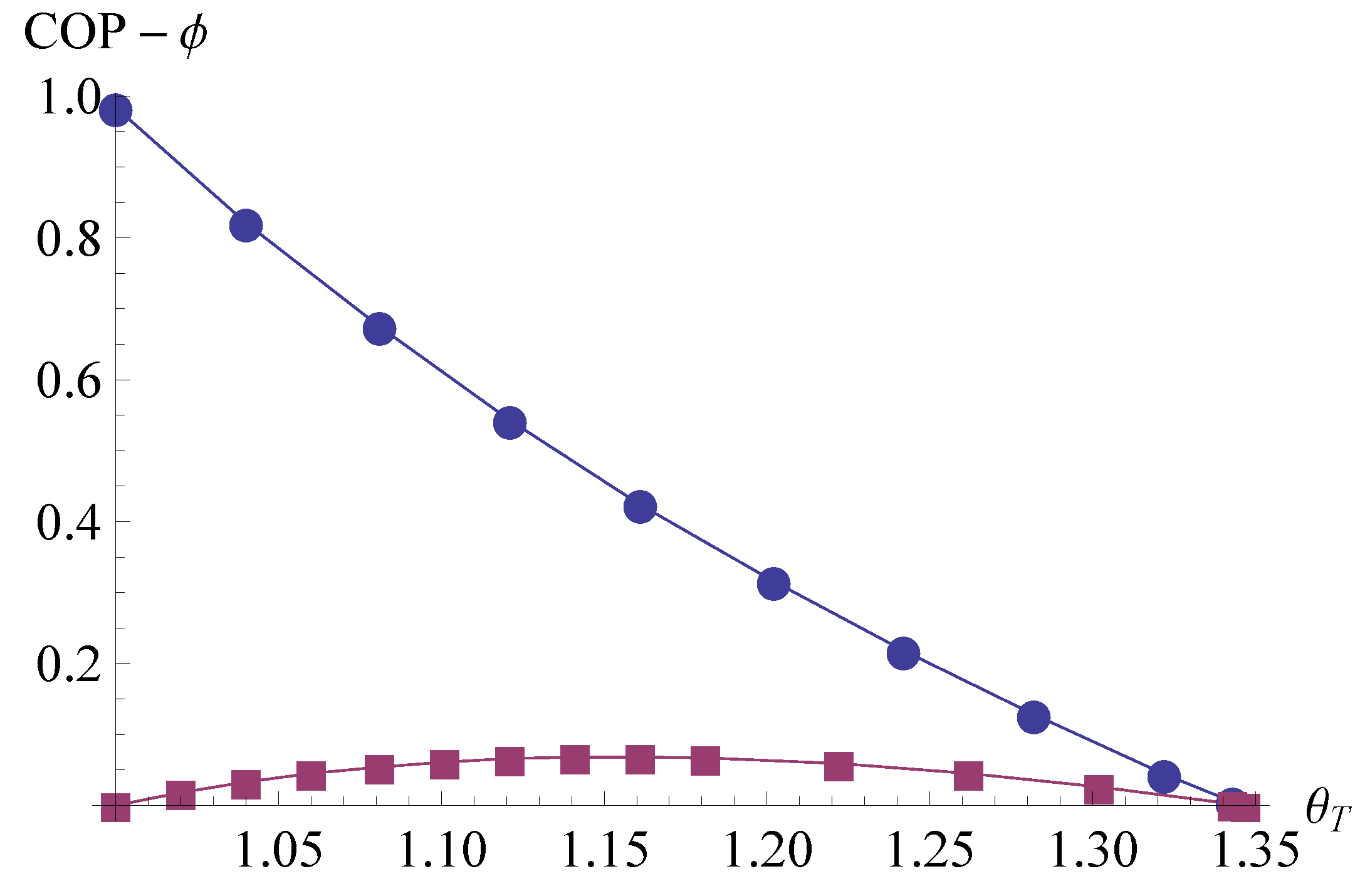Figure 2 shows clearly the above mentioned. There we have plotted the exergetic efficiency and the performance coefficient, Equations (31) and (34) respectively, against ${\theta }_T$ which is considered a measure of the temperature difference between the cold and the hot side of the TEM. Small blue circles correspond to the COP and small red squares to ϕ. It is seen in Figure 2 that the maximum of ϕ occurs at about ${\theta }_T=1.18$.

Figure 2. COP (Equation (34)) and ϕ (Equation (31)) vs.${\theta }_T=T_{H_1}/T_{C_2}$. Blue circles correspond to COP and red squares to ϕ. The difference $T_{H_1}-T_{C_1}$ increases as ${\theta }_T$ increases. $j_1=0.095$ and $j_2=0.4141$. COP-ϕ means COP or ϕ.

Before analyzing expression (31) for the exergetic efficiency, we firstly specify the values of the parameters involved in the calculations and secondly we define the ideal value of current for stage 2 (see Figure 1). The Seebeck coefficients of the p and n-type semiconductor are taken as ${\alpha }_p={\alpha }_n=1.8\times {10}^{-4}\frac{V}{K}$ , the thermal conductivities as ${\kappa }_p={\kappa }_n=1.4\times {10}^{-2}\frac{W}{Kcm}$ and the electrical resistivity as ${\rho }_p={\rho }_n=7.7\times {10}^{-4}\Omega cm$. The temperature of the cold side of the TEM is taken as $T_{C_2}$ = 248 K. The resulting hot side temperature from the maximum condition for the exergetic efficiency is $T_{H_1}$ = 308 K. Since the parameters R and K always appear as a product in Equations (14)–(16) and (21), it is needless to assign values to the cross section S and the length of the arm l (see Equations (1) and (3)).

Now we define the ideal current $j_{2max}$ as the value of $j_2$ which corresponds to the maximum exergetic efficiency. We derive Equation (31) with respect to $j_2$ and by equating it to zero we get for $j_2$ the simple expression

$$j_{2max}=Z{T}_{C_2}$$

(35)

This means that the maximum ϕ with respect the current flowing in the upper stage depends only on the thermoelectric properties of its semiconductor material and the temperature $T_{C_2}$ of the cold side of the TEM. The value of $j_{2max}$ is $0.4141$ when the thermoelectric data above mentioned is used in Equation (14). This value will be introduced in the further calculations.

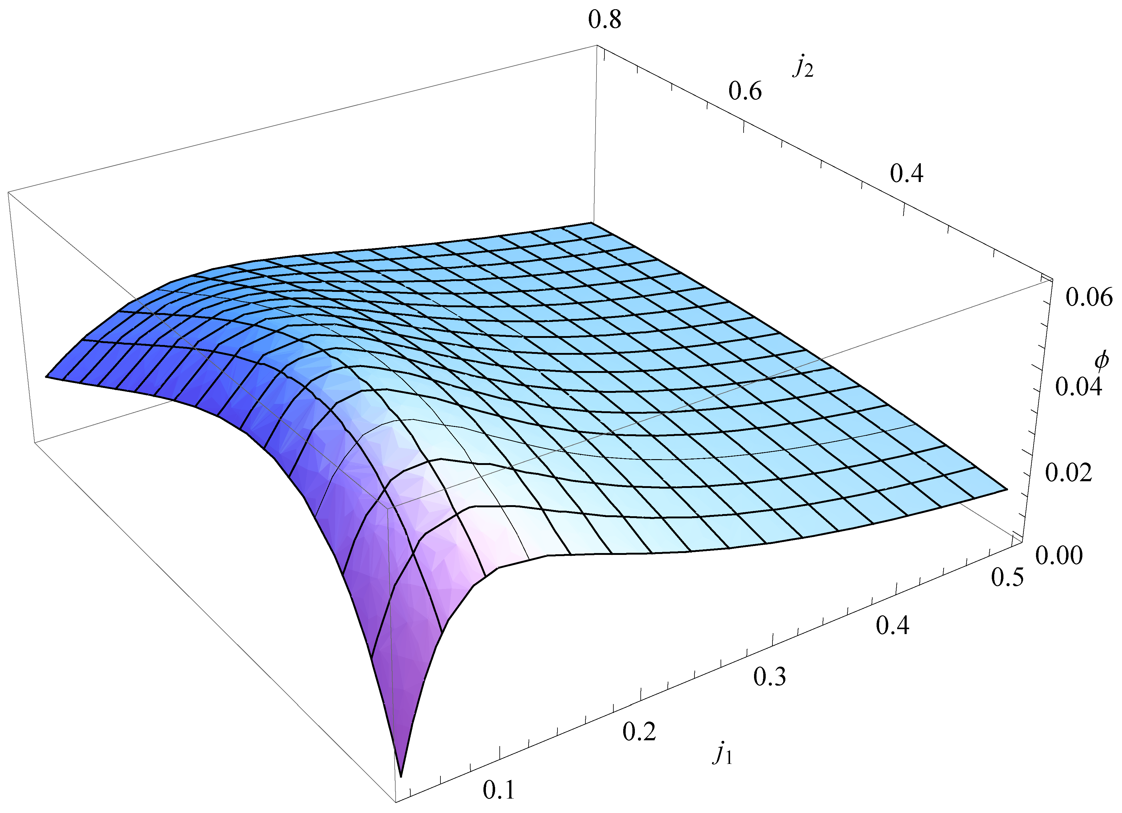
In a 3D plot, Figure 3 shows the behavior of the ϕ as a function of the dimensionless currents $j_1$ and $j_2$. Observe the maximum occurring at the ideal value $0.4141$ of $j_2$ and at $j_{1max}$ determined through the condition $d\varphi /d{j}_1=0,$ then solved for $j_1$. The solution is a cumbersome function of $j_2$ and the set of thermoelectric parameters of the system and the temperatures $T_{C_2}$ and $T_{H_1}$ obtained with the aid of Mathematica. It is not going to be shown here. When the value of $j_{2max}$ is substituted together with the above data in the solution we get $j_{1max}=0.095$ when $n_1=10$ and $n_2=1,$ i.e., when $r=10.$

Figure 3. ϕ (Equation (31)) vs.$j_1$ and $j_2,$ the currents flowing through stages 1 and 2, respectively. $T_{C_2}=248K,$$T_{H_1}=308K$. The maximum of ϕ is at $j_1=0.095$ and $j_2=0.4141$, $r=10$.

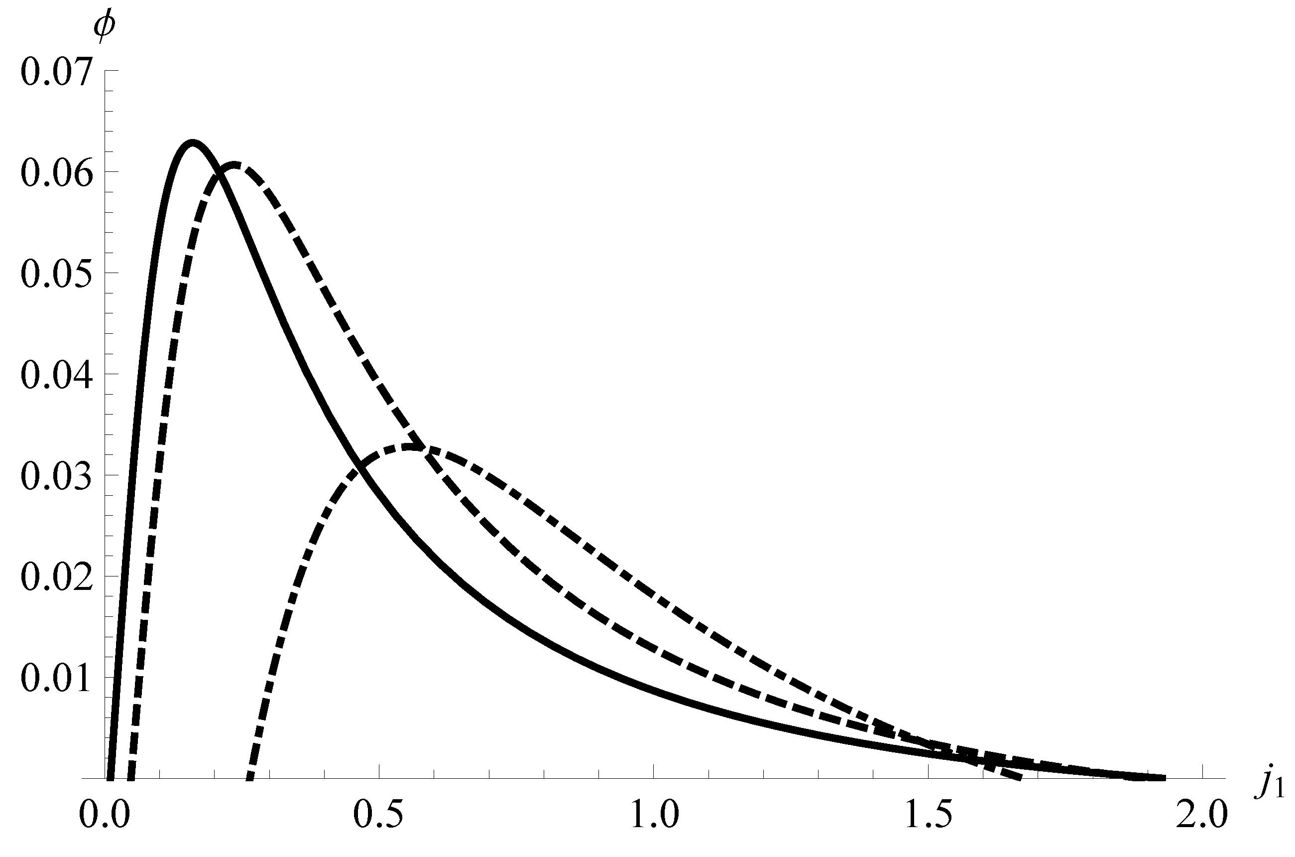
In Figure 4 we display the dependence of the ϕ on the current $j_1$ for three different numbers $n_1$ of thermocouples in the stage 1, always with $n_2=1$. We take the ideal value for $j_{2max}=0.4141$. We remark the following facts. First, it is seen that the maxima of the ϕ with respect to $j_1$ are shifted to the left as the value of $n_1$ increases. Second, the ϕ decays faster with the current $j_1$ when the value of $n_1$ increases. Third, the maximum value of the ϕ increases as $n_1$ increases and soon reaches a kind of saturation value. 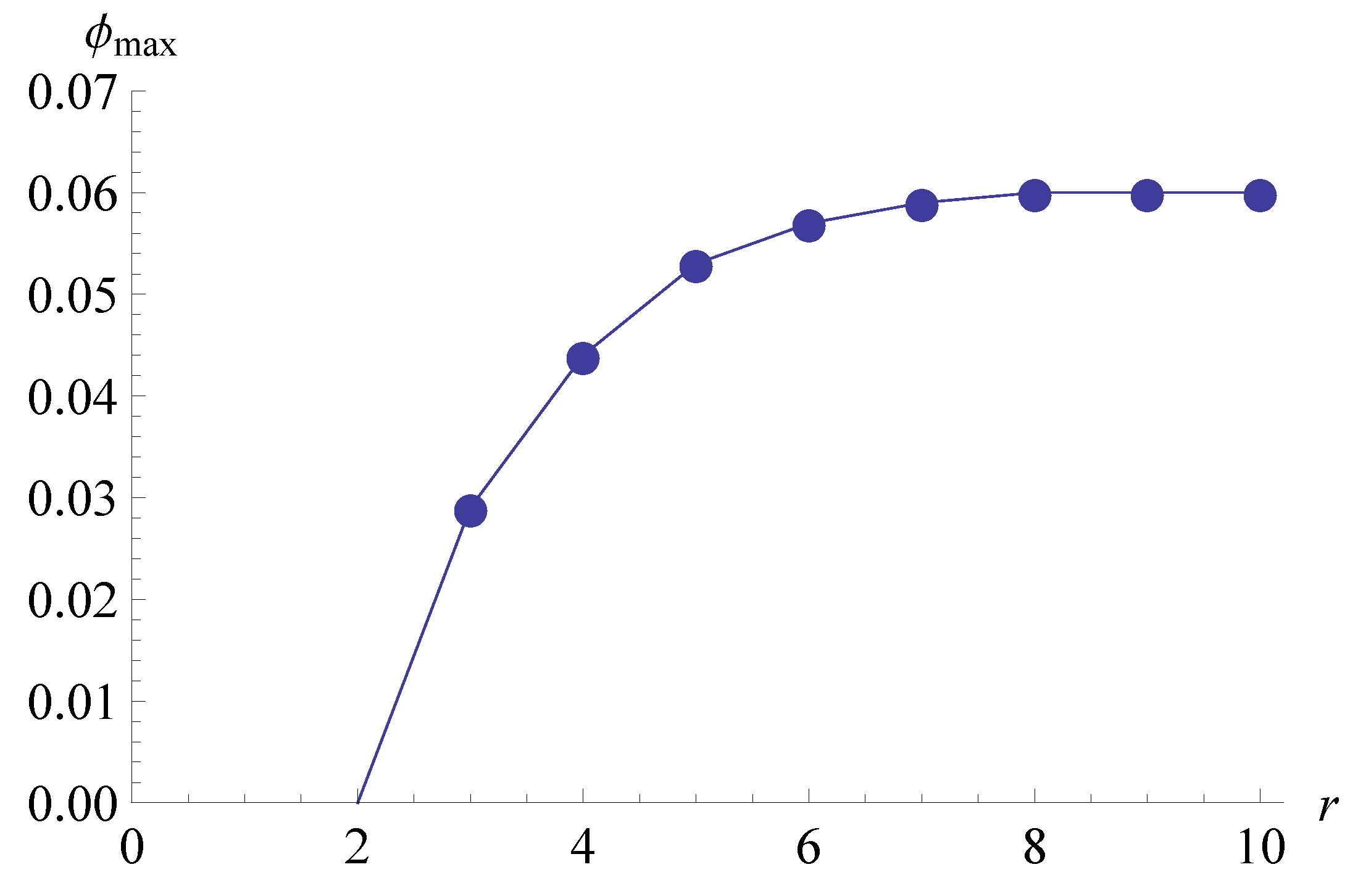This last fact can not be seen in Figure 4 but we show it in Figure 5 where we plot the behavior of the maximum ϕ as a function of the ratio r. For $r<1$, Figure 5 was obtained with $n_1=1$ and $n_2=5,4,3,2$. For $r\ge 1$ we took $n_2=1$ and $n_1=1,2,3,4,5,...,10$. The value of saturation is $0.06$ which is reached for $r=8$. It is worth noting the fact that for $n_1=8$ and $n_2=1$, not only the bigger value of ϕ is obtained for $j_1=j_{1max}$ and $j_2=j_{2max}$ among the possible combinations $(n_1,n_2)$, but it also shows positive values throughout the range of values considered for $j_1$. The effects of r on $j_{1max}$ are not shown here but it must be mentioned that $j_{1max}$ decreases as r increases. Clearly, it is preferable to design the TEM with the prescription that $n_1>n_2$ but the ratio $n_1/n_2$ does not need to be bigger than 8. Another interesting result is obtained by graphing the ϕ vs. the Seebeck coefficient of semiconductor material in stage 1.

Figure 4. ϕ (Equation (31)) vs.$j_1$ for different structures of the TEM. Solid line: $n_1=5$, $n_2=1$; dashed: $n_1=3$, $n_2=1$; dot-dashed: $n_1=1$, $n_2=1$. $j_2=j_{2max}=0.4141,$$T_{C_2}=248K,$$T_{H_1}=308K$. The maximum of ϕ moves to the left when the number of thermocouples in stage 1 increases.

Figure 5. ${\varphi }_{max}$ vs.r. $j_2=j_{2max}=0.4141$, $T_{C_2}=248K,$$T_{H_1}=308K$. The figure shows the saturation value of ${\varphi }_{max}$ when the number of thermocouples in stage 1 increases.

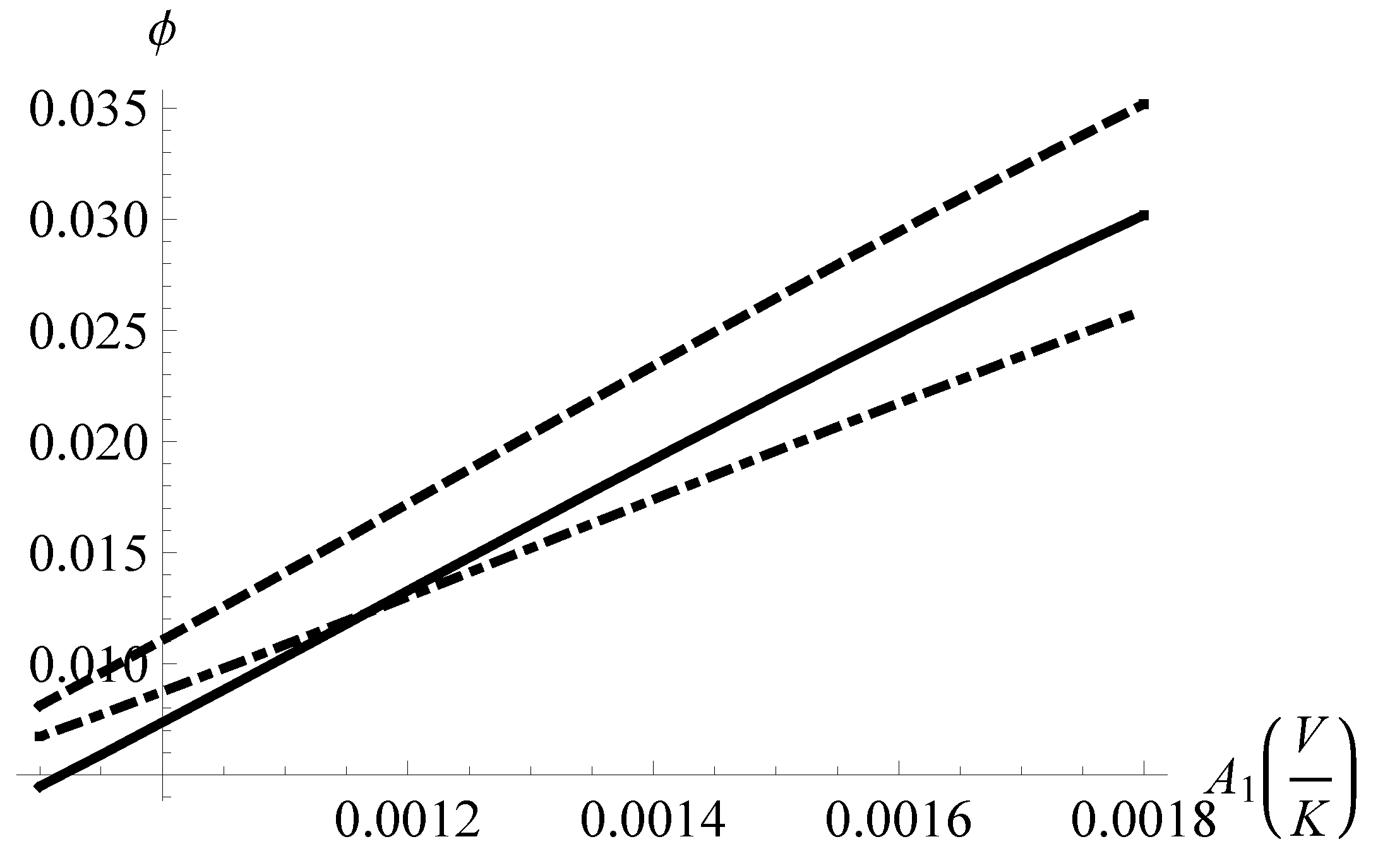
In Figure 6 the dependence of ϕ with respect to the Seebeck coefficient A of stage 1, Equation (2), is shown for several temperature differences $\Delta T$ ($=T_{H_1}-T_{C_2}$) between the cold and hot sides of the TEM (see the details in the caption of Figure 6). Besides remarking that by increasing the Seebeck coefficient we get better performances, we mention that the position of each curve can be understood in terms of Figure 2. Solid line corresponds to ${\theta }_T=1.24$, i.e., to the right of the maximum of ϕ in Figure 2 and dot-dashed line corresponds to ${\theta }_T=1.08$, i.e., to the left of the maximum. Finally, the electric resistance R (Equation (1)) and the heat conductivity K (Equation (3)) should be decreased in order to get better performances. We end this section by comparing the exergetic efficiency considered in this paper with that obtained when the two flowing electric currents, $j_1$ and $j_2$ in stages 1 and 2 respectively, have the same value [15]. We have plotted in Figure 7 the maximum value of ϕ from our results (blue circles) and the case when $j_1=j_2$ (red circles). All the remaining parameters have been kept without change. We remark that the efficiency in the first case is up to a factor of 2 bigger than the second one. In the following section we make a discussion and get some conclusions.

Figure 6. ϕ(Equation (31)) vs.$A_1$, the Seebeck coefficient of thermocouples in stage 1, for different temperature differences. Solid line: $\Delta T=60K,$ dashed: $\Delta T=40K,$ dot-dashed: $\Delta T=20K.$$j_1=0.095$, $j_2=0.4141$.

Figure 7. ${\varphi }_{max}$ vs.${\theta }_T$, for two cases. Red circles: $j_1$ equal to $j_2$ and blue circles: $j_1$ and $j_2$ have different values. All the remaining parameters are kept the same in the two cases. The exergetic efficiency has higher values when the flowing currents have different values.

4. Discussion and Conclusions

We have analyzed the exergetic efficiency of a two stage thermoelectric cooler. Four factors determine the performance of the TEM measured by ϕ: (1) the structure defined by the ratio r which was defined as the ratio of the number of thermocouples in stage 1 and stage 2; (2) the flowing electric currents in stages 1 and 2; (3) the thermoelectric properties of the thermocouples of each stage A, R and K; and (4) the difference of temperatures $\Delta T$ between the cold side and the hot side of the TEM. The existence of an optimum ϕ as a function of the electric currents flowing in stages 1 and 2 was confirmed as may be verified in Figure 3 for given structure and thermoelectric properties of the semiconductor materials. The optimal value of $j_2$ does not depend on the structure nor the operating temperatures. It only depends on the merit figure $Z{T}_{C_2}$ through the simple relation given by Equation (35); i.e., it depends only on the thermoelectric properties of stage 2. It follows that $j_1$ is a function of r (structure) and ${\theta }_T$ (operating temperatures), if the thermoelectric properties of stage 2 are taken as fixed by the industrial available TEM’s. This argument yields the important conclusion that all the maxima of the exergetic efficiency are found in the $j_2=j_{2max}$ plane (see Figure 3). The behavior of ϕ with respect to $j_1$ shown in Figure 4 and the fact (not shown here) that it does not have any extremum in the $(r,{\theta }_T)$ space allowed us to analyze the optimal functioning conditions of the two stage TE cooler in terms of the flowing electric currents in each stage only. Our results made evident that once $j_{2max}$ and $j_{1max}$ have been determined, it is recommended that the ratio be about 8 since no additional significant increment of ϕ can be obtained for $r>8$. In these conditions, the value $j_1=j_{1max}$ of the current flowing through the stage 1 is the smallest value at which the module works at maximum performance (mention must be made that a minimum in the temperature difference between the stages of the TEM is also reached for $r\ge 8$). This support our statement in the introduction in the sense that by allowing each stage to have its own working electric current, a better performance can be achieved (see also Figure 7). The optimal ratio $j_{2max}/j_{1max}$ is about 4.3. Finally, the geometric parameters of the thermocouples, namely, the cross area S and the length l of the p and n arms, do not influence the performance of the TEM.