Abstract
Aggregated sales forecasting is an important research topic in the highly competitive retail industry. With the availability of different data sources, various techniques and models have been proposed for aggregated sales forecasting. However, existing methods often overlook the spatial correlation in sales between neighboring retailers. In this paper, we propose a new framework for aggregated sales forecasting based on the deep learning technique ConvLSTM with an attention mechanism to solve this challenge. In the new framework, ConvLSTM is utilized to fully leverage spatially relevant information from adjacent retailers, while the attention mechanism is employed to capture spatial dependencies and select the most pertinent data from spatial inputs. Furthermore, a spatial sliding window technique is designed to augment the sample size. To validate the efficacy of our proposed framework, we conducted experiments using real-world retail sales data and compared our model with established benchmarks. Additionally, we conducted an ablation study to assess the contributions of key components, including the attention mechanism and spatial data augmentation. The experimental results demonstrate that our proposed model effectively improves the prediction performance, offering a novel approach to aggregate sales forecasting for both industry and academia.
1. Introduction
Aggregate sales forecasting is a crucial issue in retail research in the era of e-commerce. It involves constructing models to predict future sales aggregated over product units, locations, or time buckets []. Accurate forecasts of aggregate sales can help companies make sound marketing decisions. For example, it can support dynamic promotional strategies, such as live ops campaigns, ensuring sufficient stock availability during rapid online sales surges. Conversely, poor forecasting can lead to stockouts or excess inventory across both digital and physical channels, resulting in substantial operational and financial inefficiencies. Therefore, academics and industry professionals have increasingly recognized the significance of aggregate sales forecasting. Retail companies are now more dedicated to extracting valuable insights from vast data to improve their forecasting accuracy, and researchers have conducted extensive research to enhance the effectiveness of prediction models from different dimensions.
There are two primary methods to execute aggregate sales forecasting. One approach focuses on predicting a single time series representing the aggregated sales. The other approach is bottom-up, which first predicts individually and then aggregates the predictions. Nowadays, forecasting at the lower level is becoming increasingly feasible due to the availability of rich data at lower levels. Therefore, bottom-up methods are attracting considerable interest in current forecasting research for higher accuracy. However, sales from different segments are often interrelated. For example, nearby stores may have overlapping customer demands, resulting in spatial correlations between sales from neighboring subregions. However, existing aggregated sales forecasting research has rarely considered these spatial correlations. How to take the spatial correlation into consideration and improve the accuracy of aggregate sales requires further research efforts.
In this paper, we focus on aggregated sales forecasting over regions and a new forecasting framework called ASFC (Aggregated Sales Forecasting based on ConvLSTM) to fully exploit the spatial correlation information. Deep learning techniques have demonstrated their superior capability in time series forecasting tasks such as sales forecasting. Among the deep learning techniques, ConvLSTM proposed by Shi et al. [] has emerged as an excellent approach in many fields since its ability to deal with complex spatio-temporal dependencies. Therefore, we integrate ConvLSTM with an attention mechanism to design a framework that adopts a bottom-up methodology for aggregate forecasting. Specifically, the target area is divided into grids. Then, an enhanced SA-ConvLSTM structure is built to train the data sequence. ConvLSTM employs convolutional operations instead of Hadamard products in LSTM to facilitate the extraction of spatial patterns. An attention mechanism captures the dependency relationships between different parts of the input sequence []. A novel spatial sliding window technique is designed to augment and smooth the data to avoid data scarcity due to empty sales in certain grids. Finally, sales forecasts from each grid are aggregated to produce the overall prediction. To evaluate the performance of ASFC, we conducted extensive experiments on real-world data from a retail company and benchmarked our framework against several established methods. The results showed that ASFC outperformed all baseline approaches. Furthermore, we performed an ablation study to isolate and assess the contributions of key components, including the attention mechanism, and the spatial sliding window. This analysis demonstrates that integrating these components significantly improves spatial and temporal modeling capabilities, ultimately leading to superior forecasting performance.
The main contributions of this paper are as follows:
- A new way is explored to improve the accuracy of aggregate sale forecasting in retail by capturing spatial correlations. To the best of our knowledge, little research has considered the spatial correlations in aggregate forecasting, not to mention aggregate sales forecasting.
- A new deep learning-based framework is designed for sales forecasting. The framework integrates ConvLSTM network and attention mechanism in an encoder-decoder structure to fully exploit the information of spatial correlation. Meanwhile, a spatial data augmentation technique is introduced to address the issue of data scarcity.
2. Literature Review
2.1. Sales Forecasting in Retail
In recent years, numerous methods have emerged for sales forecasting. All the methods can be broadly classified into two categories: statistical-based approaches and machine-learning approaches.
2.1.1. Statistical-Based
Historical approaches to sales forecasting frequently relied on statistical techniques. Based on historical sales data, time series analysis and its optimization models are widely used in sales forecasting. These models include but are not limited to, single exponential smoothing (SES) [] and auto-regressive integrated moving average (ARIMA) []. Several innovations focus on modeling trends and seasonal patterns in single-variable time series data. For example, Van Calster et al. defined a flexible profit function and proposed a seasonal ARIMA model to forecast sales volume []. Choi et al. fused the classical SARIMA method with the wavelet transform for a novel hybrid approach []. Moreover, Ding and Li developed an optimized grey model to predict electric vehicles (EVs) sales and stock []. Wu et al. proposed a Bayesian model based on a non-homogeneous Poisson process with a Gaussian process prior to accurately forecast online product sales by capturing complex multi-trend patterns and addressing distribution shifts [].
2.1.2. Machine Learning
Machine learning techniques have significantly contributed to advancements in sales forecasting. For example, Castillo et al. used several machine learning algorithms such as Decision Trees, K-nearest Neighbors (KNN), Support Vector Machines (SVM), and Linear Regressions to predict the sales of new books []. Karmy and Maldonado also exploited Support Vector Regressions in a hierarchical manner to forecast European travel retail sales []. Furthermore, Chen and Lu employed the segmentation of training data through clustering, followed by the application of various machine learning techniques to create group-specific predictive models for computer retailing []. Li et al. proposed an exponential decomposition machine for sales forecasting, integrating novel product attributes with pairwise interactions []. Shao et al. proposed a hybrid machine learning approach for forecasting Chinese new energy vehicle (NEV) sales by integrating sentiment analysis, data decomposition, and machine learning models []. Wellens et al. proposed a simplified yet effective tree-based machine learning framework for retail forecasting that outperforms traditional statistical methods while maintaining computational efficiency []. These machine learning strategies have significantly increased the accuracy of sales forecasts.
2.1.3. Deep Learning
Recently, deep learning methods have demonstrated numerous successful applications in sales forecasting, driven by the continuous increase in the volume and complexity of data. The strength of deep learning lies in its immense computational capacity and ability to capture complex interrelationships among various factors. For instance, Ma and Fildes introduced a meta-learning framework based on deep convolutional neural networks in forecasting retail sales []. He et al. proposed a novel approach based on long short-term memory with particle splinter optimization (LSTM-PSO) for sales forecasting in E-Commerce companies []. Pan and Zhou utilized CNNs for online sales forecasting based on data from Alibaba, and their method yielded better results than ARIMA models []. Li et al. proposed a combined method using GRU, Prophet and attention mechanisms to predict clothing sales []. Efat et al. proposed a hybrid sales forecasting model that combines adaptive trend estimated series (ATES) with a deep neural network based on a GRU-CNN-LSTM architecture to capture dynamic and nonlinear sales patterns at the product-specific store level []. Liu et al. proposed a hybrid electric vehicle sales forecasting method combining BERT-BiLSTM-based sentiment analysis and secondary decomposition []. Wu et al. proposed a two-stage deep learning approach that is based on the online channel consumer preference heterogram and multi-head attention mechanism to enhance multi-channel retail sales forecasting []. Zhang et al. proposed a temporal fusion transformer (TFT)-based multimodal framework to enhance sales forecasting in the live-streaming e-commerce market []. de Castro Moraes et al. proposed stacked (S-CNN-LSTM) and parallel (P-CNN-LSTM) hybrid architectures to model complex time series data in retail selling forecasting [].
2.2. Aggregated Forecasting
Over the past few years, aggregated forecasting has garnered considerable attention and has been successfully investigated in various domains, including load forecasting and retail forecasting. Currently, the methods of aggregated forecasting can be categorized into two groups: fully aggregated and fully disaggregated methods.
The traditional aggregate forecasting approach directly uses historical data at the aggregation level. One may first aggregate the data at the individual level to produce an aggregated time series and then run a forecasting model to compute the aggregate prediction. For example, Aye et al. used twenty-six single and combined forecasting models to forecast South Africa’s aggregate seasonal retail sales []. Sreekumar et al. proposed a novel probabilistic aggregated Net-Load forecasting model based on Markov Chain Monte Carlo Regression []. Bouktif et al. have developed an LSTM-RNN-based univariate model to forecast the aggregated demand of France metropolitans in short- and medium-term time horizons []. Muñoz et al. evaluated the Dynamic Mode Decomposition (DMD) algorithm for short-, medium-, and long-term aggregated energy demand forecasting [].
With the prevalence of low-level data, one may compute individual forecasts and then aggregate them. For example, Stepen et al. predicted aggregated residual load by aggregating the forecasts from all constituent premise loads on the network in a bottom-up manner []. Terui and Li applied the topic model to aggregated data to decompose a product’s daily aggregated sales volume into sub-sales for several topics []. Next, the market response regression model for each topic is estimated and aggregated.
Besides these two categories of methods. Some have also explored other innovative methods to enhance the performance of aggregate forecasting. One way is to include disaggregate information in the aggregate methods. For instance, Hendry and Hubrich forecasted the United States aggregate inflation by including the aggregate and disaggregate sectoral component data in the VAR model []. Carson et al. analyzed the aggregate demand for commercial air travel in the United States, where disaggregated information in airport-specific data is considered []. Another rising trend is the usage of clustering-based methods, where individual entities are grouped according to their patterns, and the different groups are predicted upon separately and eventually aggregated into a final forecast. For instance, Cini et al. proposed a novel approach for predicting the aggregated load of a set of meters, taking cluster-level aggregates of load profiles as inputs []. Han et al. proposed a day-ahead load forecasting method that aggregates residential smart meter data, where residential consumers are clustered into several groups using the K-means algorithm based on their consumption characteristics []. Eandi et al. presented spatio-temporal graph neural network models that use cluster-level smart meter data and their spatial relationships to improve electricity demand forecasting [].
Fully aggregated methods overlook fine-grained low-level information. Fully disaggregated methods or adding disaggregated information to aggregated methods utilize such fine-grained information, but they fail to consider the correlation of individual time series. Clustering-based methods partly alleviate these issues by exploiting similarities in individual patterns, but they still mainly focus on temporal dependencies rather than modeling spatial interactions. In contrast, our work explicitly incorporates spatial correlation into the forecasting process. We propose a framework that captures both temporal dependencies and spatial interactions between neighboring retail regions. Compared with existing aggregate and disaggregate forecasting methods, our approach provides a novel perspective for improving aggregated sales forecasting in retail.
3. Methodology
3.1. Framework
Aggregated sales forecasting involves predicting the consolidated sales of these aggregated entities, grouped by unit, location, or region. This paper focuses primarily on aggregated sales forecasting for retailers across various regions. More specifically, we forecast the total sales of all retailers selling a specific type of product in the target region as follows:
where represents the total sales, and represents the sales of the i-th sub-region. The sales of adjacent subregions and are usually highly correlated because the adjacent retail stores often share customer demand.
In this paper, we focus on the research question: How to make full use of spatial correlation to improve the accuracy in aggregate sales forecasting. Existing methods commonly treat subregions in isolation, neglecting the interdependence. We propose a bottom-up framework named ASFC, which aims to address the overlooked spatial correlation between neighboring retail areas in aggregate sales forecasting. ASFC explicitly models these spatial dependencies by integrating the strengths of ConvLSTM and attention mechanisms, capturing both spatial relationships and temporal dynamics in the forecasting process, which provides a new structure design for the sales forecasting.
The ASFC framework consists of three main components as illustrated in Figure 1: spatial feature extraction, SA-ConvLSTM-based process modeling, and forecast combination. The target area is first divided into grid cells, with retail sales data from each cell forming a temporal feature sequence. During spatial feature extraction, a spatial sliding window is employed for data augmentation, helping to alleviate sparsity and enhance spatial continuity. These sequences are then fed into the SA-ConvLSTM network, which jointly models spatial and temporal patterns. Finally, in the forecast combination stage, predictions from all grid cells are aggregated to produce the overall sales forecast.
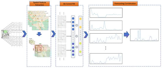
Figure 1.
Overview of the ASFC framework.
By incorporating both fine-grained grid-level modeling and spatial context across neighboring regions, the ASFC framework provides a more accurate and robust solution for regional aggregate sales forecasting. The following two subsections describe in detail the spatial feature extraction process and the architecture of the SA-ConvLSTM network.
3.2. Spatial Feature Extraction
During the spatial feature extraction stage, the target area is divided into a grid of cells of equal size. By computing the sales within each cell, we obtain a feature map represented by a matrix . Repeating this process for T time steps, we derive a 3D tensor with dimensions . Instead of feeding the initial feature map into the SA-ConvLSTM based network, we employ a sliding window across the spatial dimension to augment the data as shown in Figure 2. Specifically, we use a sliding step size along the latitude and longitude directions to generate new samples. For example, we can slide the top-left corner of an original sample by one unit along the latitude and one unit along the longitude to produce a new sample. During this process, samples that consistently showed zero sales are removed. The spatial sliding window will enrich and smooth the training data.
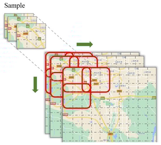
Figure 2.
Spatial sliding window.
3.3. SA-ConvLSTM Based Modeling
During modeling, we construct a deep neural network structure based on the ConvLSTM network and the attention mechanism. Figure 3 shows the overall architecture of the proposed SA-ConvLSTM-based model, which adopts an encoder–decoder structure with a central SA-ConvLSTM module to capture spatiotemporal dependencies. The encoder consists of stacked convolutional and transposed convolutional layers followed by a group normalization layer, aiming to extract high-level spatial features from the input. The core SA-ConvLSTM module alternately stacks ConvLSTM and self-attention layers, enabling the model to jointly learn temporal dynamics and focus on important spatial regions. The decoder mirrors the encoder, using convolutional and transposed convolutional layers to reconstruct the output sequence, and generates the final predictions through a readout layer.
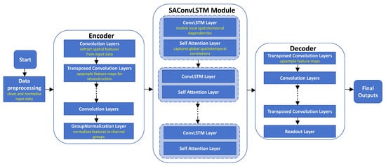
Figure 3.
Network architecture of the SA-ConvLSTM based modeling. The network architecture follows an encoder–decoder design with a central SA-ConvLSTM block. The encoder extracts spatial features, the SA-ConvLSTM learns temporal patterns while highlighting key regions, and the decoder reconstructs the final forecast.
The SA-ConvLSTM module ensures extracting vital regional information and then assimilates this into the data aggregated from prior steps. Combining the ConvLSTM model with the attention mechanism enhances the capture of spatial correlations within the input feature map to make it focus on essential parts among the heterogeneous correlations. Figure 4 presents the internal structure of the SA-ConvLSTM module, which combines a standard ConvLSTM unit with a spatial attention mechanism to enhance spatiotemporal representation learning. The ConvLSTM component first processes the input , previous hidden state , and cell state through gated convolutions to capture local temporal dynamics and generate an intermediate hidden state . This intermediate state is then fed into the attention module, where it is projected into query, key, and value representations to compute attention weights that emphasize important spatial regions. The refined output is obtained by applying these weights to the value features and integrating the result with the ConvLSTM output, enabling the model to focus on salient spatial features while maintaining temporal continuity.
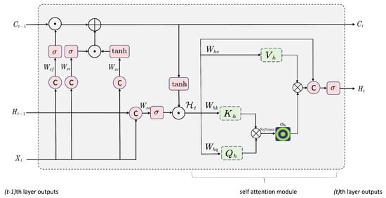
Figure 4.
Internal structure of the SA-ConvLSTM module. The ConvLSTM is responsible for modeling the temporal dynamics, while the spatial attention mechanism highlights the most informative regions. Their integration yields enhanced spatiotemporal representations that improve forecasting performance.
ConvLSTM utilizes convolutional operations for the state-to-state and input-to-state transmission instead of Hadamard products to enhance the capture of spatial correlations within the input feature map while preserving the merits of LSTM to capture long-term temporal dependencies. The main computation of ConvLSTM involves the inputs , hidden states , cell states , the input gate , output gate and forget gate . All of them can be represented as 3D tensors and computed in the following equations:
where “∗” represents the convolution operation, “·” represents the Hadamard product and W denotes a 2D convolution kernel.
The spatial attention module filters relevant information and selects the most pertinent spatial inputs. Spatial attention module first allocates weights for every spatial location within the input sequence of feature maps by analyzing patterns across space, emphasizing crucial features that significantly affect the prediction process. The spatial attention weight for every location is determined utilizing the following formula:
where denotes the attention weight for the position of the i-th spatial location, denotes the hidden state of the spatial location, and score(,) assesses the significance of each spatial location. The soft-max function will be used to compute this score. Spatial attention emphasizes recognizing the most significant spatial correlation. These attention weights are pivotal in enhancing model accuracy, allowing processes to enhance output estimates by prioritizing key information. The spatial attention module then generates a context vector by calculating the weighted average of the given spatial input variables. The context vector is intended as a weighted aggregation of the input data as follows:
The context vector can maintain crucial context by processing the entire spatial input. Finally, the obtained context vector is fed into the decoder layers to yield the final result.
4. Experimental Framework
To validate our model, we performed extensive experiments using real-world datasets. In this section, we outline the data preprocessing steps, the experimental settings, and the evaluation metrics.
4.1. Datasets
In this study, real-world data obtained from the retail industry were used for the experiments. The dataset was obtained from a fast-moving consumer goods retail network in the area , located in the eastern part of China. The original dataset contains 822,543 transaction records from 6,302 retail stores. For each transaction, the main variables include customer/store codes, geographic coordinates, store attributes, transaction amounts, and timestamps. These transaction records span the period from June to December 2019, covering 184 days. After aggregation, we obtain the sales data for each store and the total aggregated sales amount for the entire area. At the aggregate level, the daily sales have a mean of approximately 5.42 million, a median of 5.45 million, and a standard deviation of about 1.13 million. For the geographic coordinate, the longitude and latitude of each store were standardized as in Equations (9) and (10).
where and represent the standard deviation of and respectively. and represent the mean of and .
4.2. Experimental Settings
We divided the dataset into three subsets: a training set, a validation set, and a test set. The validation and test sets were both set to approximately 15% of the total dataset, while the training set comprised the remaining 70% samples. This partitioning ensures that sufficient data is available for model training, hyperparameter tuning, and performance evaluation. A moving (or rolling) window technique with 10 days was used for one-step-ahead forecasting, where the sales amounts of the previous ten periods (i.e., ) were used to forecast the sales one day ahead t. To form a feature map, we established grids with a length of 0.2. We used a sliding step size of 0.1 for longitude and latitude. More experimental results with different grid size and step size can been found in the Table A1 and Table A2 in Appendix A.
A benchmark comparison and ablation study were conducted to evaluate the ASFC model. In the benchmark comparison, fully aggregated, disaggregated methods and graph-based methods were considered. We selected SARIMA, Prophet, LightGBM, an RNN, and LSTM as our baseline, which have been extensively employed in previous studies. SARIMA is a seasonal extension of ARIMA that models both non-seasonal and seasonal patterns using autoregression, differencing, and moving averages. Prophet is a time series forecasting model that decomposes data into trend, seasonality, and holiday components, offering robust performance and interpretability for business-related forecasts. LightGBM is a gradient-boosting framework known for its speed and efficiency in handling large datasets. RNN and LSTM are neural networks specifically designed for processing sequential data. We divided the benchmark methods into two groups. In the fully aggregated group, all five methods were used to forecast sales using the aggregated data. For the disaggregated methods group, grid division approaches were exploited, which divided the whole area into grids. We obtained the final forecast by combining the individual forecasts in each grid, without considering spatial correlation. LSTM, LightGBM, and RNN were included in this group. For the graph-based methods, spatial-temporal graph convolutional networks (ST-GCN) proposed by Yan et al. were considered [], where each store was considered as a node. In the ablation study, three variants of ASFC are considered. They either ignore the sliding window, attention mechanism, or encoder-decoder structure.
In our experiments, the main hyperparameters for the proposed ASFC model included (the number of hidden units), (the number of hidden layers), (the batch size), and (the number of attention units). These parameters were evaluated with the following values: ; ; ; and . A grid search strategy was employed to systematically explore the parameter space. Based on this tuning process, the optimal configuration was determined as follows: the number of hidden units was set to 64, the number of hidden layers to 8, the batch size for training to 256 (with validation and test batch sizes of 128), and the number of attention units to 32. In addition, the convolution kernel size was fixed at (3, 3), the model was trained using the Adam optimizer with a learning rate of 0.001, and training proceeded for up to 100 epochs with EarlyStopping applied.
Additionally, we developed a series of benchmark models with tailored configurations to ensure their optimal performance under comparable conditions. Specific configurations of benchmark models are listed below. All experiments were conducted using Python with the PyTorch, Prophet, Statsmodels, LightGBM, Scikit-learn and mmskeleton packages. The experiments were run on a workstation equipped with an NVIDIA GeForce RTX 4090D GPU.
- SARIMA: Number of non-seasonal autoregressive terms, differences, and moving average terms, , seasonal order = 7;
- PROPHET: Daily frequency and seasonality with periods ;
- RNN: Number of layers = 5; Hidden units = 300;
- LSTM: Number of layers = 5; Hidden units = 300;
- LightGBM: Number of leaves = 10; Number of estimators = 500; Max depth = 8;
- ST-GCN: Number of layers = 10; batch size = 64; learning rate = 0.01; Optimizer = Adam.
4.3. Evaluation Metrics
To assess the ASFC model’s performance, we utilized the root mean square error (RMSE), mean absolute error (MAE), and mean absolute percentage error (MAPE) as evaluation metrics. These metrics gauge the disparity between forecast and actual sales in the test dataset. A lower RMSE, MAE, or MAPE indicates a more accurate forecast. The equations for calculating RMSE, MAE, and MAPE are presented below:
where is the actual sales data and is the predicted value.
5. Experimental Results
In this section, we report the experimental results and perform a comprehensive benchmark study and ablation analysis to demonstrate the effectiveness of the ASFC model for aggregated forecasting.
5.1. Benchmarking Study
Figure 5 illustrates the prediction results of our model on the TA dataset. The vertical axis represents the aggregated sales amounts, while the horizontal axis denotes all time points within the dataset. The green curve depicts the actual values, and the red curve shows the predicted values of our model. As shown in Figure 5, despite some deviations, the proposed model can effectively fit the general trend of the actual sales and gives an accurate prediction, which provides guidance for sales forecasting and offers auxiliary decision-making support for retail sales. It is also worth noting that since the missing annual cycles, our prediction is smoother, some local peaks are not predicted very accurately.
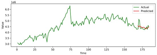
Figure 5.
Comparison between forecasting values and actual values.
Table 1, Table 2 and Table 3 present the RMSE, MAE, and MAPE values in the test sets for all the benchmark methods. The optimal value in each column is highlighted in bold. Figure 6 and Figure 7 further vividly illustrate the RMSE, MAE, and MAPE values. From the presented tables and figures, the experimental results yield several crucial insights.

Table 1.
Experimental performance of benchmark methods (Fully aggregated methods).
Table 2.
Experimental performance of benchmark methods (Fully disaggregated methods).
Table 3.
Experimental performance of benchmark methods (Graph-based methods).
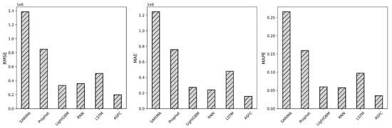
Figure 6.
Comparison between ASFC and fully aggregated benchmark methods.
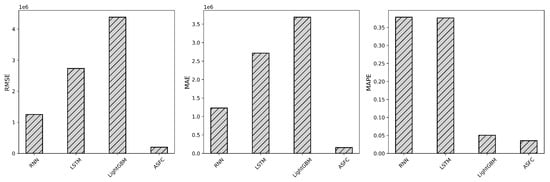
Figure 7.
Comparison between ASFC and fully disaggregated benchmark methods.
- First, we compare ASFC with fully aggregated benchmark methods. As shown in Table 1, our proposed ASFC approach achieves the highest prediction accuracy across all evaluation metrics, demonstrating its excellent performance in terms of prediction accuracy and generalization ability for ASF tasks. Applying the spatial feature extraction and the SA-ConvLSTM modelling process can capture the spatio-temporal relationship in the sequence data. Thus, the prediction error of the ASFC model is low. LightGBM and RNN yield similar results, but they perform slightly worse than ASFC. LightGBM performs slightly better than RNN. Notably, compared with LightGBM, the RMSE, MAE, and MAPE of the ASFC model improved over 40.48%, 42.19%, and 40.89%, respectively. LSTM produces slightly poorer prediction results. We believe this outcome is due to the lack of effective structures in both LSTM and RNN models to fully utilize spatial information. The Prophet performs slightly better than SARIMA but still exhibits poor overall performance, as it focuses solely on temporal patterns and fails to account for spatial correlations. In contrast, our ASFC model utilizes SA-ConvLSTM to effectively capture and strengthen the spatial and temporal dependencies in time series data. The results validate that the ASFC model achieves outstanding performance for aggregate sales forecasting.
- Secondly, we compare ASFC with fully disaggregated benchmark methods. As shown in Table 2, the highest prediction accuracy across RMSE and MAE is still achieved by our ASFC. Regarding the MAPE value, ASFC is slightly superior to LightGBM, but it significantly outperforms the other two models. With regard to RMSE and MAE, RNN and LSTM come second and third. LightGBM results in the worst performance. Interestingly, although LightGBM performs relatively well on MAPE, its RMSE and MAE are noticeably worse. This can be explained by the fact that LightGBM tends to fit low-sales grids more accurately, leading to lower percentage errors and thus a better MAPE. However, for high-sales grids or periods with sharp demand peaks, LightGBM produces larger absolute errors. Since RMSE and MAE are more sensitive to such large deviations, particularly in high-volume observations, these metrics highlight the model’s limitations in capturing fluctuations. Overall, the results confirm that our ASFC model offers a more balanced and accurate prediction across multiple evaluation metrics. Our model outperforms the other models for grid-based disaggregated methods, demonstrating its superior ability to capture spatial features.
- Next, we compare ASFC with the graph-based method. As shown in Table 3, for all three measures, ASFC has better performance than ST-GCN. When we further compare SG-GCN with fully disaggregated benchmark methods, we can see that ST-GCN does not necessarily perform better than the fully disaggregated benchmarks. For RMSE and MAE, it only beats LightGBM and is worse than RNN or LSTM. With regard to MAE, ST-GCN underperforms two of the three disaggregated benchmarks but slightly outperforms the other one.
- Finally, we compare the benchmark methods in the fully disaggregated group with thecounterpartsnce in the fully aggregated group. Interestingly, forecasting aggregated sales by combining individual forecasts at the lower level does not necessarily ensure improved performance. Sometimes, it may lead to performance deterioration. Take LSTM and RNN for example, all three measures become worse when using disaggregated rather than aggregated information. LightGBM only has slightly better performance in terms of MAPE (from 0.0597 in the fully aggregated group to 0.0504 in the fully disaggregated group), where its accuracy decreases for RSME and MAE. All this evidence shows that it is reasonable to consider the spatial correlation properly.
In summary, the consistently lower RMSE, MAE, and MAPE values of the ASFC framework compared to other methods underscore its superiority in prediction accuracy, attesting to its efficacy in improving forecast precision.
5.2. Ablation Study
The attention mechanism, spatial sliding windows, and the encoder-decoder are three important components of the ASFC. Table 4 and Figure 8 compare the performance of ASFC with its three variants, and each ignores one crucial part. We can draw several interesting conclusions from Table 4 and Figure 8.
Table 4.
Experimental performance of ablation methods.
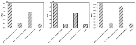
Figure 8.
Comparison between ASFC and its variants.
- First of all, the ASFC outperforms the others on all three metrics, demonstrating that the spatial sliding window, attention mechanism, and encoder-decoder module are indispensable for the model’s prediction capability.
- The encoder-decoder module achieves the most significant improvements. ASFC shows improvements of 83.08%, 86.31%, and 82.81% in RMSE, MAE, and MAPE, compared to the simple SA-ConvLSTM network structure without encoder-decoder. These results indicate that the encoder-decoder of ASFC integrates temporal and spatial information into effective embeddings for the SA-ConvLSTM architecture, enhancing the performance of the ASFC approach.
- The second most significant increase is due to the attention mechanism. ASFC shows improvements of 73.33%, 77.51%, and 81.08% in RMSE, MAE, and MAPE, respectively. These results underline the significance of the attention mechanism in enhancing the model’s ability to capture crucial spatial-temporal correlations. By focusing on the most relevant features within the data, the attention mechanism enables the ASFC model to achieve superior accuracy and robustness in its predictions.
- For the sliding window, ASFC shows improvements of 19.28%, 12.41%, and 13.7% in the three evaluation metrics. These results indicate that including sufficient and appropriately structured input data further improves the predictive performance of the ASFC model, highlighting the importance of leveraging well-prepared data for training and inference.
6. Conclusions
In today’s competitive marketplace, retail and e-commerce companies place increasing emphasis on accurately forecasting and analyzing product sales to remain competitive. For retailers, precise aggregated sales forecasts provide insights into the broader demand landscape across regions and fulfillment zones. Such forecasts not only support the formulation of effective sales and promotion strategies but also optimize inventory allocation, enhance regionalized delivery capacity planning, and improve overall profitability. Although a wide range of forecasting techniques have been proposed in academia, most overlook the spatial correlations that naturally exist among neighboring retail and e-commerce regions.
To address this gap, we employ a bottom-up forecast strategy for aggregated sales across entire regional retail landscapes, incorporating spatial correlations. We introduce the ASFC framework, a ConvLSTM network enhanced with an attention mechanism. This design emphasizes capturing vital spatial correlation data during the forecasting process. This approach is particularly beneficial for applications such as regional demand pooling, live-ops promotion planning, and fulfillment zone optimization. Extensive experiments conducted on real-world retail sales data demonstrate that the ASFC framework consistently outperforms benchmark models, achieving the lowest RMSE, MAE, and MAPE values. These results underscore the model’s superior predictive accuracy and confirm the significant spatial interdependence between sales from neighboring retailers, e-commerce platforms, and fulfillment regions.
From a theoretical perspective, our study offers a new perspective to enhance aggregated sales forecasting by emphasizing the value of incorporating spatial correlation. In addition, we present a new deep learning based architecture that integrates a ConvLSTM network and an attention mechanism in an encoder-decoder structure, tailored to the aggregated sales forecasting task. From a practical perspective, ASFC provides a data-driven decision-support tool that enhances forecasting accuracy for regional and operations managers, enabling more efficient inventory planning, delivery capacity coordination, and alignment of online and offline channels. Moreover, although the current evaluation is based on a single dataset due to data unavailability, the framework is designed for a general scenario, where aggregated sales/demand forecasting is performed over regions with spatial correlations. No other constraint is considered. The new framework jointly models temporal dependencies and spatial interaction. Therefore, it can be readily generalized to other geographic regions, retail formats, and industries.
The current ASFC framework has certain limitations: First, the overall model complexity is high, which may pose challenges in terms of training efficiency and real-time deployment in resource-constrained environments. Although all the computation can be handled on standard workstations, distributed computing resources or advanced hardware such as NVIDIA GPU may be needed to reduce the computation time. Second, the presented ASFC operates as a black box, limiting its interpretability—an aspect that is increasingly important in business contexts.
Future work could explore strategies to reduce model complexity, such as lightweight network designs or model compression techniques. Enhancing model interpretability is another promising direction—for example, by integrating explainable AI methods (e.g., Shapley-based explanations) to identify which spatial regions or time steps most influence the forecast. In addition, conducting extensive experiments on more datasets can further verify the generalizability of our method to other datasets or domains. Incorporating exogenous variables (e.g., weather, promotions, demographics) could also validate its generalizability and practical relevance.
Author Contributions
Conceptualization, K.L. and D.X.; methodology, B.Z.; software, Z.S.; validation, B.Z. and S.v.B.; formal analysis, Z.S.; investigation, K.L.; resources, B.Z.; data curation, B.Z.; writing—original draft preparation, B.Z.; writing—review and editing, B.Z., Z.S. and S.v.B.; visualization, Z.S.; project administration, B.Z.; funding acquisition, B.Z. and S.v.B. All authors have read and agreed to the published version of the manuscript.
Funding
This work is supported by the Fundamental Research Funds for the Central Universities (Grant No. SXYPY202337).
Institutional Review Board Statement
Not applicable.
Informed Consent Statement
Not applicable.
Data Availability Statement
The dataset presented in this article is not readily available due to commercial confidentiality agreements.
Conflicts of Interest
The authors declare no conflicts of interest.
Appendix A. Sensitive Analysis of Grid and Step Size
Table A1.
Sensitive analysis of grid size.
Table A1.
Sensitive analysis of grid size.
| Grid Size | RMSE | MAE | MAPE |
|---|---|---|---|
| (16, 16) | 2.562 | 2.098 | 0.0404 |
| (20, 20) | 1.975 | 1.576 | 0.0353 |
| (24, 24) | 1.887 | 1.589 | 0.0413 |
Table A2.
Sensitive analysis of step size.
Table A2.
Sensitive analysis of step size.
| Step Size | RMSE | MAE | MAPE |
|---|---|---|---|
| (0.05, 0.05) | 1.890 | 1.532 | 0.0389 |
| (0.1, 0.1) | 1.975 | 1.576 | 0.0353 |
| (0.2, 0.2) | 3.348 | 3.012 | 0.1013 |
References
- Fildes, R.; Ma, S.; Kolassa, S. Retail forecasting: Research and practice. Int. J. Forecast. 2019, 38, 1283–1318. [Google Scholar] [CrossRef]
- Shi, X.; Chen, Z.; Wang, H.; Yeung, D.Y.; Wong, W.K.; Woo, W.c. Convolutional LSTM network: A machine learning approach for precipitation nowcasting. In Proceedings of the Advances in Neural Information Processing Systems, Montreal, QC, Canada, 7–12 December 2015; pp. 802–810. [Google Scholar]
- Vaswani, A.; Shazeer, N.; Parmar, N.; Uszkoreit, J.; Jones, L.; Gomez, A.N.; Kaiser, Ł.; Polosukhin, I. Attention is all you need. In Proceedings of the Advances in Neural Information Processing Systems, Long Beach, CA, USA, 4–9 December 2017; Volume 30. [Google Scholar]
- Li, C.; Lim, A. A greedy aggregation–decomposition method for intermittent demand forecasting in fashion retailing. Eur. J. Oper. Res. 2018, 269, 860–869. [Google Scholar] [CrossRef]
- Ramos, P.; Santos, N.; Rebelo, R. Performance of state space and ARIMA models for consumer retail sales forecasting. Robot.-Comput.-Integr. Manuf. 2015, 34, 151–163. [Google Scholar] [CrossRef]
- Van Calster, T.; Baesens, B.; Lemahieu, W. ProfARIMA: A profit-driven order identification algorithm for ARIMA models in sales forecasting. Appl. Soft Comput. 2017, 60, 775–785. [Google Scholar] [CrossRef]
- Choi, T.M.; Yu, Y.; Au, K.F. A hybrid SARIMA wavelet transform method for sales forecasting. Decis. Support Syst. 2011, 51, 130–140. [Google Scholar] [CrossRef]
- Ding, S.; Li, R. Forecasting the sales and stock of electric vehicles using a novel self-adaptive optimized grey model. Eng. Appl. Artif. Intell. 2021, 100, 104148. [Google Scholar] [CrossRef]
- Wu, Z.; Chen, X.; Gao, Z. Bayesian non-parametric method for decision support: Forecasting online product sales. Decis. Support Syst. 2023, 174, 114019. [Google Scholar] [CrossRef]
- Castillo, P.A.; Mora, A.M.; Faris, H.; Merelo, J.; García-Sánchez, P.; Fernández-Ares, A.J.; De las Cuevas, P.; García-Arenas, M.I. Applying computational intelligence methods for predicting the sales of newly published books in a real editorial business management environment. Knowl.-Based Syst. 2017, 115, 133–151. [Google Scholar] [CrossRef]
- Karmy, J.P.; Maldonado, S. Hierarchical time series forecasting via support vector regression in the European travel retail industry. Expert Syst. Appl. 2019, 137, 59–73. [Google Scholar] [CrossRef]
- Chen, I.F.; Lu, C.J. Sales forecasting by combining clustering and machine-learning techniques for computer retailing. Neural Comput. Appl. 2017, 28, 2633–2647. [Google Scholar]
- Li, C.; Cheang, B.; Luo, Z.; Lim, A. An exponential factorization machine with percentage error minimization to retail sales forecasting. ACM Trans. Knowl. Discov. Data (TKDD) 2021, 15, 1–32. [Google Scholar] [CrossRef]
- Shao, J.; Hong, J.; Wang, M.; Wang, X. New energy vehicles sales forecasting using machine learning: The role of media sentiment. Comput. Ind. Eng. 2025, 201, 110928. [Google Scholar] [CrossRef]
- Wellens, A.P.; Boute, R.N.; Udenio, M. Simplifying tree-based methods for retail sales forecasting with explanatory variables. Eur. J. Oper. Res. 2024, 314, 523–539. [Google Scholar] [CrossRef]
- Ma, S.; Fildes, R. Retail sales forecasting with meta-learning. Eur. J. Oper. Res. 2020, 288, 111–128. [Google Scholar]
- He, Q.Q.; Wu, C.; Si, Y.W. LSTM with particle Swam optimization for sales forecasting. Electron. Commer. Res. Appl. 2022, 51, 101118. [Google Scholar] [CrossRef]
- Pan, H.; Zhou, H. Study on convolutional neural network and its application in data mining and sales forecasting for E-Commerce. Electron. Commer. Res. 2020, 20, 297–320. [Google Scholar] [CrossRef]
- Li, Y.; Yang, Y.; Zhu, K.; Zhang, J. Clothing sale forecasting by a composite GRU–Prophet model with an attention mechanism. IEEE Trans. Ind. Inform. 2021, 17, 8335–8344. [Google Scholar] [CrossRef]
- Efat, M.I.A.; Hajek, P.; Abedin, M.Z.; Azad, R.U.; Jaber, M.A.; Aditya, S.; Hassan, M.K. Deep-learning model using hybrid adaptive trend estimated series for modelling and forecasting sales. Ann. Oper. Res. 2024, 339, 297–328. [Google Scholar]
- Liu, J.; Pan, H.; Luo, R.; Chen, H.; Tao, Z.; Wu, Z. An electric vehicle sales hybrid forecasting method based on improved sentiment analysis model and secondary decomposition. Eng. Appl. Artif. Intell. 2025, 150, 110561. [Google Scholar] [CrossRef]
- Wu, J.; Liu, H.; Yao, X.; Zhang, L. Unveiling consumer preferences: A two-stage deep learning approach to enhance accuracy in multi-channel retail sales forecasting. Expert Syst. Appl. 2024, 257, 125066. [Google Scholar] [CrossRef]
- Zhang, Q.; Li, X.; Gao, P. Forecasting Sales in Live-Streaming Cross-Border E-Commerce in the UK Using the Temporal Fusion Transformer Model. J. Theor. Appl. Electron. Commer. Res. 2025, 20, 92. [Google Scholar] [CrossRef]
- de Castro Moraes, T.; Yuan, X.M.; Chew, E.P. Hybrid convolutional long short-term memory models for sales forecasting in retail. J. Forecast. 2024, 43, 1278–1293. [Google Scholar] [CrossRef]
- Aye, G.C.; Balcilar, M.; Gupta, R.; Majumdar, A. Forecasting aggregate retail sales: The case of South Africa. Int. J. Prod. Econ. 2015, 160, 66–79. [Google Scholar] [CrossRef]
- Sreekumar, S.; Khan, N.; Rana, A.; Sajjadi, M.; Kothari, D. Aggregated net-load forecasting using markov-chain monte-carlo regression and C-vine copula. Appl. Energy 2022, 328, 120171. [Google Scholar] [CrossRef]
- Bouktif, S.; Fiaz, A.; Ouni, A.; Serhani, M.A. Optimal deep learning LSTM model for electric load forecasting using feature selection and genetic algorithm: Comparison with machine learning approaches. Energies 2018, 11, 1636. [Google Scholar] [CrossRef]
- Muñoz, M.C.; Peñalba, M.A.; González, A.E.S. Analysis of aggregated load consumption forecasting in short, medium and long term horizons using dynamic mode decomposition. Energy Rep. 2024, 12, 1000–1013. [Google Scholar] [CrossRef]
- Stephen, B.; Tang, X.; Harvey, P.R.; Galloway, S.; Jennett, K.I. Incorporating practice theory in sub-profile models for short term aggregated residential load forecasting. IEEE Trans. Smart Grid 2015, 8, 1591–1598. [Google Scholar] [CrossRef]
- Terui, N.; Li, Y. Measuring large-scale market responses and forecasting aggregated sales: Regression for sparse high-dimensional data. J. Forecast. 2019, 38, 440–458. [Google Scholar] [CrossRef]
- Hendry, D.F.; Hubrich, K. Combining disaggregate forecasts or combining disaggregate information to forecast an aggregate. J. Bus. Econ. Stat. 2011, 29, 216–227. [Google Scholar] [CrossRef]
- Carson, R.T.; Cenesizoglu, T.; Parker, R. Forecasting (aggregate) demand for US commercial air travel. Int. J. Forecast. 2011, 27, 923–941. [Google Scholar] [CrossRef]
- Cini, A.; Lukovic, S.; Alippi, C. Cluster-based aggregate load forecasting with deep neural networks. In Proceedings of the 2020 International Joint Conference on Neural Networks (IJCNN), Glasgow, UK, 19–24 July 2020; IEEE: New York, NY, USA, 2020; pp. 1–8. [Google Scholar]
- Han, D.; Bai, H.; Wang, Y.; Bu, F.; Zhang, J. Day-ahead aggregated load forecasting based on household smart meter data. Energy Rep. 2023, 9, 149–158. [Google Scholar] [CrossRef]
- Eandi, S.; Cini, A.; Lukovic, S.; Alippi, C. Spatio-temporal graph neural networks for aggregate load forecasting. In Proceedings of the 2022 International Joint Conference on Neural Networks (IJCNN), Padua, Italy, 18–23 July 2022; IEEE: New York, NY, USA, 2022; pp. 1–8. [Google Scholar]
- Yan, S.; Xiong, Y.; Lin, D. Spatial temporal graph convolutional networks for skeleton-based action recognition. In Proceedings of the AAAI Conference on Artificial Intelligence, New Orleans, LA, USA, 2–7 February 2018; Volume 32. [Google Scholar]
Disclaimer/Publisher’s Note: The statements, opinions and data contained in all publications are solely those of the individual author(s) and contributor(s) and not of MDPI and/or the editor(s). MDPI and/or the editor(s) disclaim responsibility for any injury to people or property resulting from any ideas, methods, instructions or products referred to in the content. |
© 2025 by the authors. Licensee MDPI, Basel, Switzerland. This article is an open access article distributed under the terms and conditions of the Creative Commons Attribution (CC BY) license (https://creativecommons.org/licenses/by/4.0/).