Determining Driving Risk Factors from Near-Miss Events in Telematics Data Using Histogram-Based Gradient Boosting Regressors

Abstract

This study introduces a novel method for driving risk assessment based on the analysis of near-miss events captured in telematics data. Near-miss events, which are highly correlated with accidents, are employed as proxies for accident prediction. This research employs histogram-based gradient boosting regressors (HGBRs) for the analysis of telematics data, with comparisons made across datasets from China and Spain. The results presented in this paper demonstrate that HGBR outperforms conventional generalized linear models, such as Poisson regression and negative binomial regression, in predicting driving risks. Furthermore, the findings suggest that near-miss events could serve as a substitute for traditional claims in calculating insurance premiums. It can be seen that the machine learning algorithm offers the prospect of more accurate risk assessments and insurance pricing.

1. Introduction

A “near miss” is considered to cause no property damage or personal injury, but is prone to damage or injury when there is a slight movement in time or location. In the field of traffic safety, near miss, also known as near accident, near collision, and so on, refers to an operation without personal or property loss but with high risk. It does not turn into an accident but from a probabilistic point of view the more near-miss events there are, the more likely it is that an accident occurs [1]. Therefore, near-miss events, which are responsible for traffic safety, are a subject of increasing interest [2]. Although near-miss events can be collected through telematics, modeling near-miss events allows us to evaluate the risk dynamically and predict potential accidents before they occur, thus enhancing preemptive safety measures. For example, a driver with a more aggressive driving style may not have a near-miss for a period of time, but the regression results of his driving data show that he does have near-miss events. In other words, regression analysis of telematics data can dig out risks hidden deep inside. In this study, a new driving risk assessment method is proposed, which uses the results of the near-miss event estimation model to calculate the driving risk of each driver. This method has been verified on datasets from China and Spain.

Vehicles and drivers are the main participants in traffic accidents, and their daily travel is inseparable from auto insurance, which provides security. Motor insurance is compulsory in most countries to protect those who should be compensated for losses caused by vehicles in motion. The premium calculation of auto insurance, which is based on the determination of claim risks and leads to insurance pricing, has always been the most concerned issue for both the policyholders and insurers. Historically, insurers have relied on the number of accidents during the insured period, in fact, insurers only consider the number of claims because policyholders may not report accidents when claiming implies that a penalization on the next term price is enforced. The reality is that, if a minor accident occurs, most of the drivers will avoid paying more premiums by not claiming [3]. Policies with no claims for several years tend to be the majority in most portfolios, making it difficult to obtain useful information that truly reflects the risks of driving [4]. With the development of telematics, usage-based insurance (UBI), a new type of vehicle insurance, can use more potential data attributes to complete the driving risk assessment and then complete the auto insurance premium determination [5]. The method of scoring driving risk based on expected near-miss events proposed in this study is a new attempt in the field of UBI. It is crucial to develop UBI systems that can provide personalized insurance premiums based on real-time driving behavior.

Research on UBI has been ongoing for years. Initially, researchers included driving mileage alongside traditional auto insurance factors to assess driving risks and set premiums. This early mileage-based approach was known as pay-as-you-drive (PAYD) [6,7,8]. Later, as data from the Internet of Vehicles became available, factors related to driving behavior and driving conditions were introduced into the rate-making model, which was called pay-how-you-drive (PHYD) [9,10,11]. In the future, if 5G communication technology and in-car processors become widely used, UBI schemes will be called manage-how-you-drive (MHYD), which will enable drivers to analyze their competence at the wheel and allow for calculating insurance premiums in real-time [12]. The driving risk assessment in this study is based on the near-miss event prediction model supported by telematics data. Still, the utilization rate of vehicles is also considered, so it should be regarded as a combination of PAYD and PHYD.

Driving risk scores are used in numerous contexts, primarily for pricing and risk analysis. This latter function can inform drivers about their performance or help insurance companies classify customers, though it is typically used internally or for marketing purposes. There are various methods for assessing driving risk. Many researchers advocate for methods based on the traditional generalized linear model (GLM), which is the most widely used in the insurance field. Linear regression [12], logistic regression [7,13], quantile regression [14], Poisson regression [15,16], zero-inflated Poisson regression [3,17], negative binomial regression [18,19], zero-inflated negative binomial regression [18,19], panel data regression [19], generalized additive model [20,21], etc., are widely used in driving risk assessment due to their good interpretability. On the other hand, black-box algorithms in machine learning have also been used in UBI research, such as cluster analysis [22,23], decision tree [7], support vector machine [24], neural network [25], gradient boosting method [26], and other relevant models [5,27]. In recent years, scholars have combined the boosted generalized linear model with machine learning to study UBI by taking advantage of both [28,29,30]. Nevertheless, the advent of these novel methodologies may encounter obstacles due to regulatory constraints in certain jurisdictions where the application of black-box predictive analysis is prohibited [31].

The role of near-miss events in driving risk assessment and premium pricing is quite flexible and can be approached from multiple perspectives. Guillen et al. [18] analyzed three types of near-miss events, i.e., cornering, braking, and accelerating, as independent variables and proved that both traditional and telematics variables are relevant to risk factors. Sun et al. [19] employed Poisson regression and negative binomial regression to analyze four types of near-miss events as dependent variables in summary datasets and panel datasets, respectively. This not only confirmed the significant influence of certain driving risk variables but also identified specific driving risk factors for each driver. Guillen et al. [4] proposed a new method for determining auto insurance rates, using historical claims as the dependent variable and near-miss events as the independent variable. They calculated influence coefficients via the log-link function and incorporated these into the pricing model to complete rate-making. Guillen et al. [32] utilized telematics data from 19,214 drivers over 55 weeks to develop predictive models for weekly accident frequency. They demonstrated that incorporating behavioral and contextual factors significantly enhances risk assessment. This approach also highlights potential usage-based insurance schemes through Poisson regression-derived driving scores and personalized safety alerts. This paper builds on previous studies but uses data that lacks information on accidents or claims. Here, the frequency of each near-miss event is treated as a dependent variable to evaluate driving risk.

The rest of this paper is organized as follows. The data structure, data description, and variable availability of the datasets from China and Spain are presented in Section 2. Section 3 presents the generalized linear model and machine learning algorithm used in this research. Section 4 presents the results of the two types of models on the two datasets. The similarities and differences are compared and discussed. Section 5 summarizes the findings and shortcomings of this study.

2. Data Description

Different telematics datasets from China and Spain are included in this study. Although the sources of the two datasets are different, their data attributes have many similarities and differences (see details in Table 1). $Harshacceleration$ ($nearmiss\_accel$) and $Harshdeceleration$ ($nearmiss\_brake$), as common attributes of the two datasets, are selected as the dependent variables of this study. It is worth noting that there are no common attributes in the driving behavior category, but they are all taken into account because they have important information about driving risk. Similarly, in the driving duration category, while $TripsinDay$ and $TripsinNight$ in the dataset from China and $nweekdays$ and $nweekenddays$ in the dataset from Spain do not appear in the other dataset, they should not be ignored because they contain key information. By the same token, in the driving distance category, $Fuel$ in the dataset from China and $distance\_max\_per\_day$, $distance\_under\_50$ kmh and $distance\_above\_120$ kmh in the dataset from Spain are retained.

Table 1. Types, names, and definitions of the data attributes from the China telematics dataset and the Spain telematics dataset.

Type	Dataset from China	Dataset from Spain	Definition
identity	ID	telematics ID	Telematics-box unique identification number
nearmiss event	Harshacceleration	nearmiss_accel	Frequency of cases when acceleration is greater than 6 m/s2
	Harshdeceleration	nearmiss_brake	Frequency of cases when acceleration is less than −6 m/s2
		nearmiss_accel_under_50 kmh	Frequency of cases when acceleration is greater than 6 m/s2 and speed is under 50 km/h
		nearmiss_brake_above_120 kmh	Frequency of cases when acceleration is less than −6 m/s2 and speed is above 120 km/h
	Overspeed		Frequency of driving speed greater than 100 km/h
	Highspeedbrake		Frequency of braking when the driving speed is greater than 90 km/h
driving behavior	Speed	speed_mean	Mean of speed (km/h)
		speed_max	Maximum of speed (km/h)
		accel_mean	Mean of acceleration (m/s2)
	Brakes		Total number of brakes
	Range		Range of driving (geographical units)
	RPM		Mean of revolutions per minute (r/min)
	Accelerator pedal position		Mean of acceleration pedal position (%)
	Engine fuel rate		Mean of engine fuel rate (%)
		headig_mean	Average distance to the vehicle in front (m)
driving duration	Days	ndays	Total number of driving days
	Trips	ntrips	Total number of driving trips that count if the vehicle remains stationary for more than five minutes
	TripperDay	ntrips_per_day_media	Number of driving trips per day
	TripsinDay		Total number of driving trips during the day
	TripsinNight		Total number of driving trips at night
	Weekdays	nweekdays	Total number of driving days in weekdays
	Weekends	nweekenddays	Total number of driving days in weekends
	TripsinWeekdays	ntrips_in_weekdays	Total number of driving trips on weekdays
	TripsinWeekends	ntrips_in_weekenddays	Total number of driving trips on weekends
	Trips ≤ 15 m	ntrips_under_15 min	Total number of trips with a driving time under 15 min
	15 m < Trips ≤ 30 m	ntrips_between_15 min_30 min	Total number of trips with a driving time of more than 15 min or less than 30 min
	30 m < Trips ≤ 1 h	ntrips_between_30 min_1 h	Total number of trips with a driving time of more than 30 min and less than 1 h
	1 h < Trips ≤ 2 h	ntrips_between_1 h_2 h	Total number of trips with driving time between 1 h and 2 h
	Trips > 2 h	ntrips_longer_2 h	Total number of trips with a driving time of more than 2 h
driving distance	Distance	distance	Total driving distance (km)
	Fuel		Total fuel consumption (L)
	DistanceperTrip	distance_per_trip_media	Driving distance per trip (km)
	DistanceinWeekdays	distance_week_media	Driving distance on weekdays (km)
	DistanceinWeekends	distance_weekend_media	Driving distance on weekends (km)
	DistanceinDay	distance_during_day	Driving distance during the day (km)
	DistanceinNight	distance_during_night	Driving distance at night (km)
		distance_max_per_day	Maximum driving distance per day (km)
		distance_under_50 kmh	Driving distance when driving speed is less than 50 km/h (km)
		distance_above_120 kmh	Driving distance when driving speed is greater than 120 km/h (km)

The two datasets have their own data structures. The main feature is that neither dataset contains accidents or claims, while frequent near-miss events can serve as valuable indicators of driving risk. Unlike accidents and claims, which occur only a few times a year, near-miss events tend to occur more frequently and are easily captured by telematics sensors. The dataset from China contains telematics data from 261 vehicles over six days, as shown in Table 2. Notice that the means of $Harshacceleration$ and $Harshdeceleration$ are both non-negative integers, which suggests that Poisson regression models could be used. In contrast, the dataset from Spain consists of 285 connected vehicles with a period ranging from 1 to 194 days, see Table 3. Notice that $nearmiss\_accel$ and $nearmiss\_brake$ are also non-negative integers but their variances are much higher than the mean, which suggests that Poisson regression may not be as good as negative binomial regression in modeling the frequency of near misses. In general, negative binomial regression would be more appropriate when there is excessive dispersion in the count data, but if this dispersion is mainly caused by a few outliers, the Poisson regression model may be more robust. In other words, the negative binomial regression model may be affected by outliers, leading to biased parameter estimates and, thus, affecting predictive performance. Note that the median, 75% quantile, and maximum value of the $speed\_max$ variable are equal, which might indicate repeated values caused by sensor errors. Consequently, this variable has been ignored in this study.

Table 2. The data description for the dataset from China includes the count, mean, standard deviation, and quartiles.

Variable	Mean	Standard Deviation	Minimum	25%	50%	75%	Maximum
Harshacceleration	139.613	162.567	0	33	80	200	1062
Harshdeceleration	198.893	199.638	1	71	133	248	1694
Brakes	1446.854	1288.607	0	621	1027	1947	9243
Speed	37.745	16.084	1.164	25.596	38.805	49.858	70.493
Range	4.511	4.533	0.0188	1.162	2.521	6.838	26.781
RPM	847.308	192.205	123.863	765.633	869.082	951.701	1375.211
Accelerator pedal position	16.981	6.825	0.187	12.551	17.392	21.326	34.127
Engine fuel rate	9.359	4.300	0.731	6.347	8.804	12.231	19.211
Days	5.494	1.047	1	5	6	6	6
Trips	39.345	17.491	3	28	38	49	102
TripperDay	7.102	2.834	1.4	5	6.667	8.667	20.400
TripsinDay	23.333	14.856	1	13	20	31	96
TripsinNight	16.011	11.125	0	7	15	23	56
TripsinWeekdays	26.556	12.205	0	19	25	33	79
TripsinWeekends	12.789	7.493	0	8	12	17	39
Trips ≤ 15 m	19.398	11.654	0	12	18	25	64
15 m < Trips ≤ 30 m	4.548	3.553	0	2	4	6	27
30 m < Trips ≤ 1 h	3.900	3.759	0	1	3	6	19
1 h < Trips ≤ 2 h	3.985	3.946	0	1	3	6	21
Trips > 2 h	7.513	4.863	0	3	7	11	23
Distance	2176.589	1561.173	18.334	882.527	1935.629	3056.883	7401.503
Fuel	559.446	430.039	10.248	258.162	420.131	843.811	2018.369
DistanceperTrip	61.266	45.742	0.796	25.931	50.391	82.575	216.569
DistanceinWeekdays	1409.925	1042.584	0	610.642	1173.935	1976.121	4941.579
DistanceinWeekends	766.664	606.723	0	266.412	748.427	1094.106	2786.403
DistanceinDay	858.247	944.155	0	105.312	545	1297.322	5082.737
DistanceinNight	1318.342	1051.073	0	484.326	1108.903	1952.406	5195.649

Table 3. The data description for the dataset from Spain includes the count, mean, standard deviation, and quartiles.

Variable	Mean	Stdandard Deviation	Minimum	25%	50%	75%	Maximum
nearmiss_accel	118.477	182.752	0	3	15	172	968
nearmiss_brake	30.782	78.487	0	0	3	24	658
speed_mean	14.293	5.324	1.614	11.059	14.168	17.729	32.617
speed_max	36.952	6.780	13.112	33.404	41.330	41.700	41.700
accel_mean	0.00527	0.0191	0	0.000602	0.00137	0.00314	0.258
headig_mean	171.628	29.237	45.033	159.537	173.564	186.139	279.689
ndays	40.888	53.767	1	2	7	70	194
ntrips	132.102	186.887	1	5	17	216	819
ntrips_per_day_media	2.703	1.141	1	2	2.739	3.308	8
nweekdays	31.179	40.785	0	1	5	55	145
nweekenddays	9.709	13.750	0	0	2	16	56
ntrips_in_weekdays	103.218	145.023	0	3	13	171	645
ntrips_in_weekenddays	29.460	46.616	0	0	5	46	228
ntrips_under_15 min	63.348	95.346	0	2	8	100	511
ntrips_between_15 min_30 min	41.018	62.884	0	1	6	58	369
ntrips_between_30 min_1 h	19.709	33.485	0	0	3	23	225
ntrips_between_1 h_2 h	5.509	10.263	0	0	1	7	68
ntrips_longer_2 h	2.519	6.416	0	0	0	2	59
distance	2,598,486	3,924,461	2202.191	60,812.701	369,717.903	4,025,068	21,416,301
distance_per_trip_media	20,254.511	16,384.724	2202.191	10,371.821	16,436.243	24,441.733	142,954.600
distance_week_media	54,322.604	62,479.617	0	19,942.939	40,155.481	66,025.783	571,818.303
distance_weekend_media	47,438.224	55,849.631	0	0	35,019.364	70,342.073	386,267.301
distance_during_night	648,796.203	1,042,995	0	10,269.070	77,628.823	909,464.704	5,305,998
distance_during_day	1,949,690	2,984,507	0	45,305.752	322,924.604	2,948,788	17,182,576

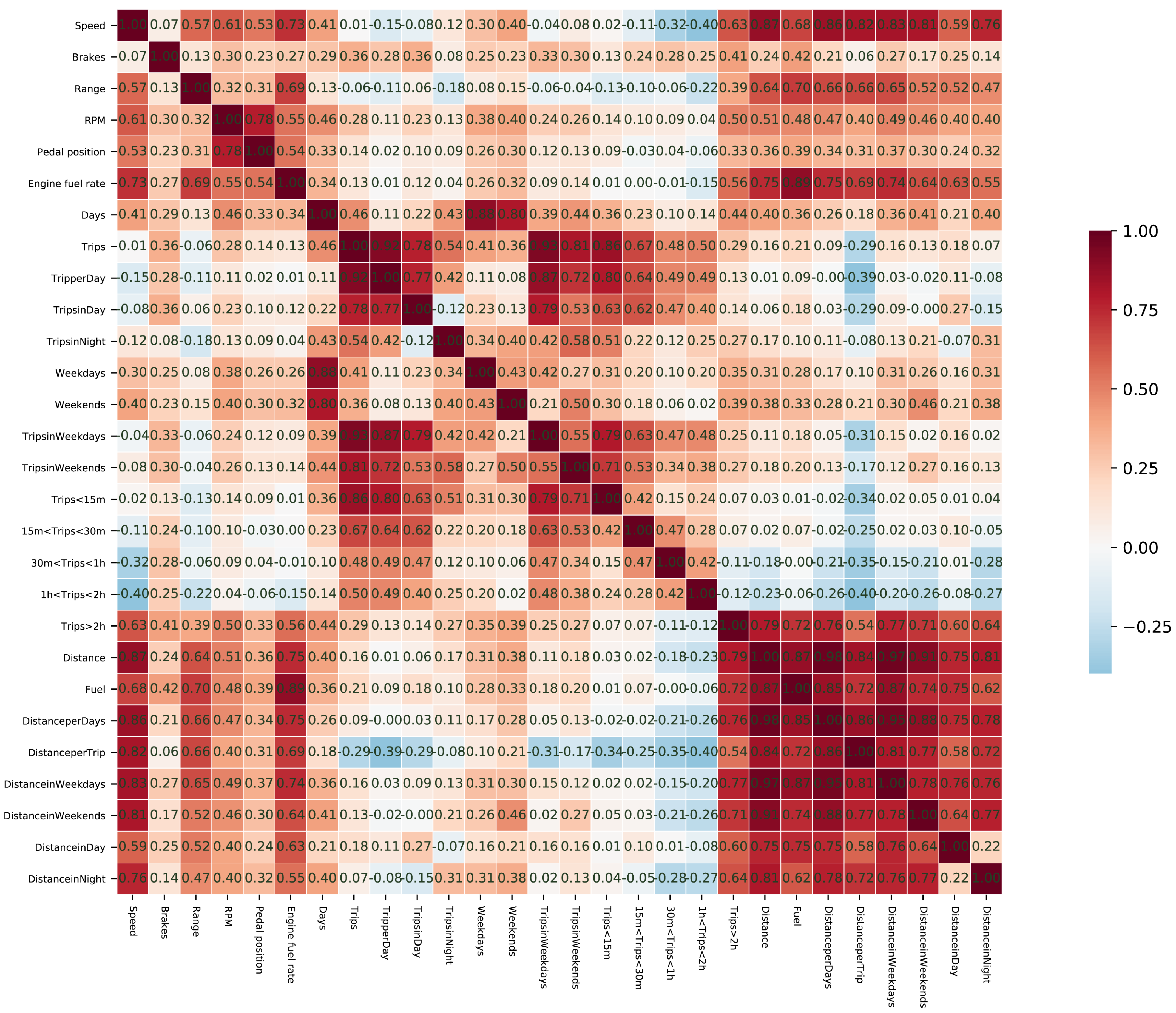
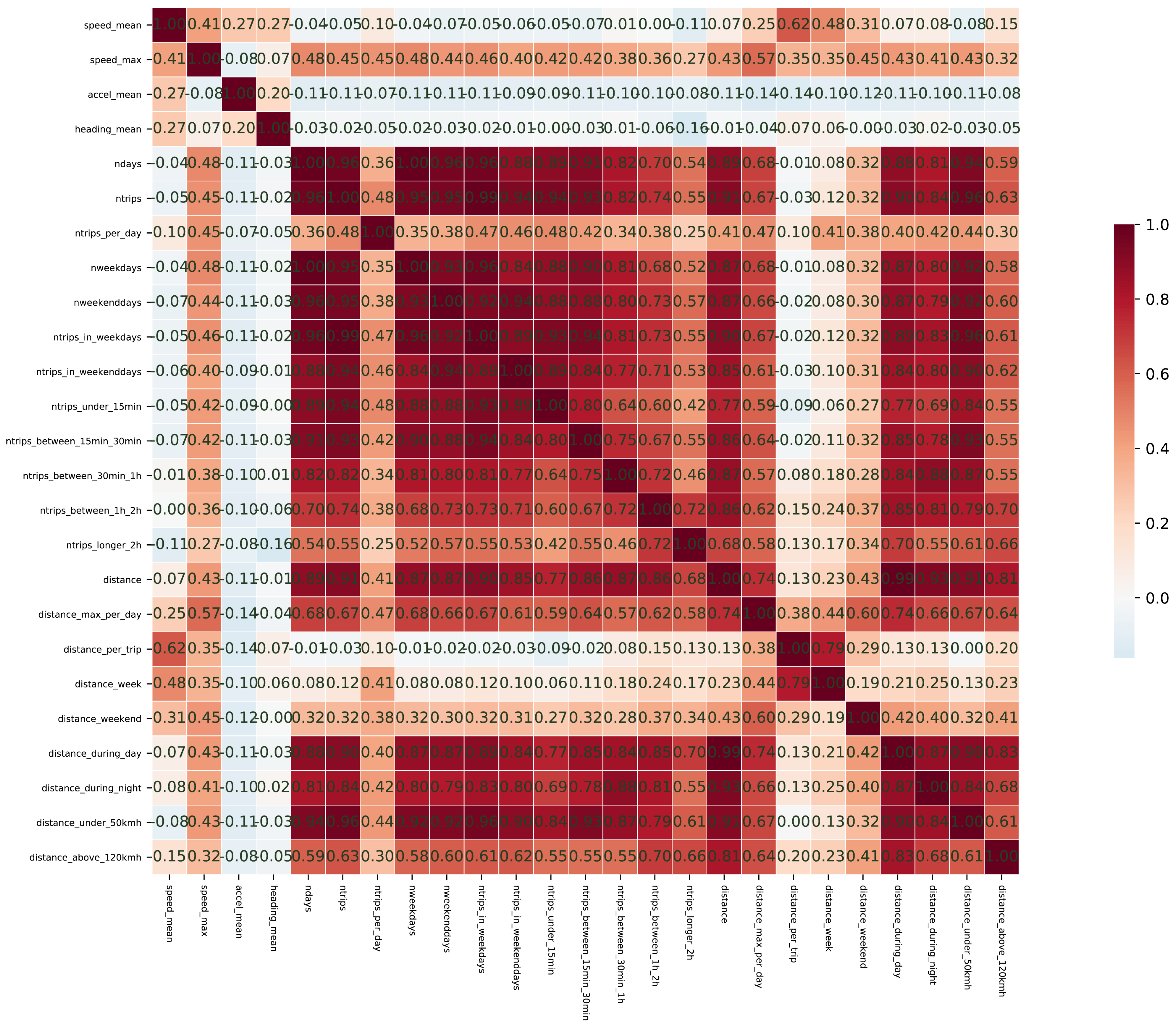
Given the large number of data attributes, a correlation analysis of the variables was also conducted prior to modeling and before examining the regression results. In the dataset from China, as shown in Figure 1, each type of variable exhibits a certain degree of internal correlation. Notably, the driving distance variables demonstrate the strongest correlation. There is a positive correlation between driving behavior variables and driving distance variables, whereas the correlation between driving duration variables and the other two types of variables is weak or even negative. In the dataset from Spain (see Figure 2), driving distance variables and driving duration variables show an obvious positive correlation, while driving behavior variables have no obvious correlation with other variables. Interestingly, the linear correlation between dependent variables and independent variables in the dataset from China is not strong, but the correlation between dependent variables and independent variables in the dataset from Spain is strong. Since the correlation between independent variables can affect model parameter identification and the assessment of causality, it is necessary to conduct multicollinearity tests and make trade-offs before modeling. Alternatively, regularization terms can be added to eliminate the bad effects of multicollinearity during modeling. As shown in Table 4 and Table 5, after eliminating variables with the excessive variance inflation factor (VIF), the remaining variables passed the multicollinearity test. Although, this work is not limited to generalized linear models, the number of variables involved in this study can be easily handled by a machine learning algorithm, which is good at processing multidimensional data.

Figure 1. Correlation of variables from the dataset from China. Red represents linear positive correlation and blue represents linear negative correlation; the darker the color, the stronger the linear correlation.

Figure 2. Correlation of variables from the dataset from Spain. Red represents linear positive correlation and blue represents linear negative correlation; the darker the color, the stronger the linear correlation.

Table 4. Variance inflation factor and inverse variance inflation factor for the dataset from China.

Variable	VIF	1/VIF
TripperDay	8.17	0.12
Speed	7.55	0.13
Trips ≤ 15 m	6.18	0.16
DistanceinWeekends	5.06	0.20
RPM	4.17	0.24
TripsinWeekends	3.77	0.27
Engine fuel rate	3.65	0.27
Trips > 2 h	3.58	0.28
Accelerator pedal position	3.27	0.31
DistanceinDay	2.62	0.38
30 m < Trips ≤ 1 h	2.40	0.42
Range	2.28	0.44
TripsinNight	2.26	0.44
1 h < Trips ≤ 2 h	2.19	0.46
15 m < Trips ≤ 30 m	2.07	0.48
Brakes	1.60	0.62
Mean VIF	3.80

Table 5. Variance inflation factor and inverse variance inflation factor for the dataset from Spain.

Variable	VIF	1/VIF
ntripsinweekenddays	8.76	0.11
distance_during_night	8.10	0.12
ntrips_under_15 min	6.32	0.16
ntrips_between_15 min_30 min	5.58	0.18
distance_per_trip	5.22	0.19
distance_week	4.82	0.21
ntrips_between_30 min_1 h	4.73	0.21
ntrips_between_1 h_2 h	4.36	0.23
distance_max_per_day	3.85	0.26
ntrips_longer_2 h	3.09	0.32
distance_above_120 kmh	2.87	0.35
speed_mean	2.72	0.37
ntrips_per_day	2.26	0.44
distance_weekend	2.15	0.47
accel_mean	1.40	0.71
headig_mean	1.15	0.87
Mean VIF	4.21

3. Methods

3.1. Modeling

Conventional GLMs are preferred and assignable in the UBI scenario [31]. In the context of a Poisson regression model, the conditional expectation function is a non-negative function of a vector of explanatory variables. This is analogous to the negative binomial regression model, where the conditional expectation function is also defined by a log-link function, as follows:

$$E(y_i\mid x_i)={\lambda }_i=T_i\times exp({\beta }_0+{\beta }_1{x}_{1i}+\cdots +{\beta }_k{x}_{ki})$$

(1)

where ${\lambda }_i$ denotes the expectation of $y_i$, i denotes the number of the observation, $T_i$ denotes the risk exposure variables, $x_{1i}$...$x_{ki}$ represent the independent variables that have passed the VIF multicollinearity test, and constant ${\beta }_0$ and ${\beta }_1$...${\beta }_k$ are unknown parameters that need to be estimated.It should be noted that to facilitate comparative analysis of the results, the exposure variables for both datasets in this study are measured in days. But, in practice, the value of the exposure variable can vary depending on the actual situation [4].

In contrast to the preceding studies, a gradient boost method is introduced to deal with the potentially large data volume in the practical work of UBI. The HGBR algorithm is an improved gradient boosting regression tree (GBRT) algorithm based on histograms [33]. The basic idea of HGBR is to discretize continuous floating-point eigenvalues into integer-valued bins and construct a histogram with the width of k. When traversing the data, the histogram accumulates statistics according to the discretized values as indices. After traversing the data once, the histogram accumulates the required statistics and then traverses according to the discrete values of the histogram to find the optimal segmentation point and build the gradient boosting tree, which tremendously reduces the number of splitting points to consider instead of relying on sorted continuous values. Hence, the HGBR algorithm offers advantages such as low memory consumption, reduced computational costs, high cache utilization rate, and a clear construction process. This is why similar iterative processes are found in algorithms like XGBoost and LightGBM [34]. It is well-known that the auto insurance industry is characterized by high-dimensional and large-volume data, and the future expansion of telematics is expected to lead to even more explosive growth in data volume and complexity. Such data characteristics meet the scope of application of the HGBR algorithm.

It is important to note that the HGBR loss function $L_t$ adds an L2 regularization term based on the traditional GBRT loss function:

$$L_t=\sum _{i=1}^{n}L[(y_i,f_{t-1}\left(x_i\right)+h_t\left(x_i\right)]+{\displaystyle \frac{\lambda }{2}}\sum _{j=1}^m{w}_{tj}^2$$

(2)

where n represents the sample size, $h_t\left(x_i\right)$ represents the output value of the tth decision tree; m represents the number of leaf nodes of the tth decision tree; $w_{tj}$ denotes the optimal value of the jth leaf node; and $\lambda$ represents the regularization coefficient. Since the output requirement of this study is non-negative, a 1/2 Poisson deviation is selected as the base loss function; see Equation (3).

$$L\left[y_i,f_{t-1}\left(x_i\right)\right]=y_{i}log{\displaystyle \frac{y_i}{f_{t-1}\left(x_i\right)}}-\left[y_i-f_{t-1}\left(x_i\right)\right].$$

(3)

Equation (2) can be obtained through a series of approximate derivations, such as the Taylor expansion, as follows:

$$L_t=\sum _{j=1}^m[G_{tj}{w}_{tj}+{\displaystyle \frac{1}{2}}(H_{tj}+\lambda )w_{tj}^2]$$

(4)

where $G_{tj}$ represents the first-order derivative of Equation (3), and $H_{tj}$ represents the second-order derivative of Equation (3). When each leaf node region takes the optimal solution $w_{tj}=-{\displaystyle \frac{G_{tj}}{H_{tj}+\lambda }}$, the minimum loss function is as follows:

$$L_t^{min}=-{\displaystyle \frac{1}{2}}\sum _{j=1}^m{\displaystyle \frac{G_{tj}^2}{H_{tj}+\lambda }}.$$

(5)

Then, the optimal split point of each leaf node region can be determined by analyzing the change in Equation (5) before and after the split. Assume that the sum of the first-order derivatives of the loss function for the parent leaf node before the split is $G_P$, and the sum of the second-order derivatives is $H_P$. After the split, the sum of the first-order derivatives for the left leaf node is $G_L$, and the sum of the second-order derivatives is $H_L$. The sum of the first-order derivatives of the right leaf node after the split is $G_P-G_L$, and the sum of the second-order derivatives is $H_P-H_L$. The loss gain before and after the node split is defined as follows:

$$Gain={\displaystyle \frac{1}{2}}{\displaystyle \frac{G_L^2}{H_L+\lambda }}+{\displaystyle \frac{1}{2}}{\displaystyle \frac{{(G_P-G_L)}^2}{H_P-H_L+\lambda }}-{\displaystyle \frac{1}{2}}{\displaystyle \frac{G_P^2}{H_P+\lambda }}.$$

(6)

The split point that maximizes Equation (6) before and after the leaf node region split is the optimal split point. The pseudocode of HGBR is shown in Algorithm 1. The HGBR process in this study is implemented with the help of sklearn.ensemble.HistGradientBoostingRegressor.

Algorithm 1 HGBR on near-miss

Input:  training set: $D=(x_1,y_1),(x_2,y_2),...,(x_n,y_n)$; loss function: $L\left[y_i,f_{t-1}\left(x_i\right)\right]=y_{i}log{\displaystyle \frac{y_i}{f_{t-1}\left(x_i\right)}}-\left[y_i-f_{t-1}\left(x_i\right)\right]$; maximum number of bins: K; regularization coefficient: $\lambda$; iteration limit: T 1: Initialization: $f_0\left(x\right)=\underset{h}{\underbrace{argmin}}{\sum }_{i=1}^{K}L(y_i,h)$ 2: repeat 3:    Construct histograms on each feature variable, calculating each bin’s first derivative sum of loss function $Hist\left[{Bin}_k\left(i\right)\right].G+={\displaystyle \frac{\partial L\left[y_i,f_{t-1}\left(x_i\right)\right]}{\partial f_{t-1}\left(x_i\right)}}$ and the second-derivative sum of the loss function $Hist\left[{Bin}_k\left(i\right)\right].H+={\displaystyle \frac{{\partial }^{2}L\left[y_i,f_{t-1}\left(x_i\right)\right]}{\partial f_{t-1}^2\left(x_i\right)}}$; 4:    By each $Bin$ as a split point, accumulate the first derivative on the left $G_L$ and the second derivative on the left $H_L$. Given the first derivative on the parent $G_P$ and the second derivative on the parent $H_P$, the first derivative on the right is $G_R=G_P-G_L$, and the second derivative on the right is $H_R=H_P-H_L$; 5:    Calculate the loss gain at each split point $Gain={\displaystyle \frac{1}{2}}{\displaystyle \frac{G_L^2}{H_L+\lambda }}+{\displaystyle \frac{1}{2}}{\displaystyle \frac{G_R^2}{H_R+\lambda }}-{\displaystyle \frac{1}{2}}{\displaystyle \frac{G_P^2}{H_P+\lambda }}$, the eigenvariable corresponding to the maximum loss gain and the eigenvalue of $Bin$ are the eigenvariable and the optimal eigenvalue of the optimal split node $w_{tk}={\underbrace{argmin}}_h{\sum }_{x_i\in R_{tk}}L\left[y_i,f_{t-1}\left(x_i\right)+h_t\left(x_i\right)\right]$, where $R_{tk}$ represents the kth $Bin$ region corresponding to the tth regression tree; $t+=1$. 6: until$t>=T$  Output:  strong learner: $F\left(x\right)=f_T\left(x\right)=f_0\left(x\right)+{\sum }_{t=1}^T{\sum }_{k=1}^K{w}_{tk}I\left(x\in R_{tk}\right)$

3.2. Driving Risk Factor

According to Chinese regulations, China’s auto insurance premium rate-making model is as follows:

$$P={\displaystyle \frac{P_{\mathrm{basic}}}{(1-r)}}\times C_{\mathrm{adjustment}}$$

(7)

where the benchmark premium $P_{\mathrm{basic}}$ is based on static characteristics such as the vehicle brand, engine capacity, driver age, ..., and the additional fee rate r is based on the additional items purchased by the policyholder, only the rate adjustment factor $C_{\mathrm{adjustment}}$ can be adjusted by the insurance company. The risk adjustment factor contains many contents, such as a traffic violation factor, a non-indemnity discount, and a driving risk score factor, which is the very focus of this study. The idea of the PAYD mode is that the more a vehicle is used, the greater the probability that accidents or near-miss events occur. Using this idea, a risk factor based on usage can be obtained as follows:

$$C_{\mathrm{usage}}=1-e^{-{\beta }_n{x}_n}$$

(8)

where $x_n$ represents a variable that measures the vehicle utilization rate, which is positively correlated with near-miss events, ${\beta }_n$ denotes the estimated value obtained by the predictive model (note that we assume that ${\beta }_n>0$), $C_{\mathrm{usage}}$ goes from 0 to 1. In this study, $x_n$ denotes the number of driving trips per day.

The relationship between originally observed and predicted risk events requires special attention. The predicted expected frequency value is the Poisson distribution expectation computed from the regression model. If the original value is greater than the predicted value, it indicates that the model underestimates the driving risk, and the driving risk factor will naturally be higher. On the contrary, if the original value is less than the predicted value, it indicates that the model overestimates the driving risk and the corresponding risk factor is low. Given the above description, and assuming that both the original values obey the Poisson distribution, the near-miss event risk factor can be obtained from the Poisson cumulative distribution function, as follows:

$$C_{\mathrm{near}-\mathrm{miss}}=\sum _{k=0}^y{\displaystyle \frac{{\widehat{y}}^k}{k!}}{e}^{-\widehat{y}}$$

(9)

where y represents the original value of near-miss events, $\widehat{y}$ represents the predicted value of near-miss events, and the $C_{\mathrm{near}-\mathrm{miss}}$ goes from 0 to 1. By adding the above two factors, the driving risk factor—considering both vehicle utilization rate and near-miss event probability—can be obtained as follows:

$$C_{\mathrm{risk}}=(1-\alpha )·C_{\mathrm{usage}}+\alpha ·C_{\mathrm{near}-\mathrm{miss}}=(1-\alpha )·(1-e^{-{\beta }_n{x}_n})+\alpha ·\sum _{k=0}^y{\displaystyle \frac{{\widehat{y}}^k}{k!}}{e}^{-\widehat{y}}$$

(10)

where $\alpha$, ranging from 0 to 1 (0.5 in this study), represents the proportion of near-miss events that are taken into account in the driving risk factor, $C_{\mathrm{risk}}$ goes from 0 to 1, the higher the value, the greater the driving risk. In practical applications, each type of risk factor can be weighted and averaged, which will not be discussed in this study.

4. Results and Discussions

Assuming that each near-miss event (as a dependent variable) obeys the Poisson distribution, the Kolmogorov–Smirnov test was conducted on them, respectively, and the test results (seeing Table 6) showed that none of the four near-miss events conformed to the standard Poisson distribution. This may bring about the estimation results of Poisson regression bias. In order to compare the effects of the two regressions, Poisson regression and negative binomial regression were estimated on the dataset from China and the dataset from Spain, respectively, and their coefficient estimations and significance results are shown in Table 7 and Table 8. It is worth noting that prior to undertaking the regressions, the independent variables were subjected to standardization. This process entailed the division of the total number of variables such as brakes, trips, and distance by the exposure period, thereby converting them into average daily rates (with the “$\_pd$” suffix). This modification was implemented to ensure that the values of the independent variables were comparable across insureds with varying exposure periods, thereby enhancing the robustness and interpretability of the model. From the regression results, whether in the dataset from China or Spain, most of the independent variables in the Poisson regression demonstrate significant effects, regardless of which near-miss event is used as the dependent variable. However, it seems to mean that the variances of the estimators are probably understated. Furthermore, the Akaike information criterion (AIC) and Bayesian information criterion (BIC) of negative binomial regressions are smaller than Poisson regressions for the same variables. The log-likelihood of the negative binomial regression is higher than that of the Poisson regression. And the discrete parameter $\alpha$ is significantly greater than zero. These all imply that the negative binomial regression performs more convincingly at the parameter estimation level relative to Poisson regression. Since this study focuses more on obtaining an accurate prediction model, further validation is needed to compare the accuracy of the two predictions.

Table 6. Kolmogorov–Smirnov test for four near-miss events.

Variable		Harshacceleration	Harshdeceleration	Nearmiss_Accel	Nearmiss_Brake
N		261	261	285	285
Poisson parameter	mean	139.612	198.889	118.483	30.784
	absolute	0.617	0.584	0.641	0.710
Most extreme differential	positive	0.617	0.584	0.641	0.710
	negative	−0.290	−0.274	−0.287	−0.159
Kolmogorov–Smirnov Z-value		9.975	9.432	10.823	11.989
Asymptotic significance (two-tailed)		0	0	0	0

Table 7. Results of Poisson regression and negative binomial regression for the variables Harshacceleration and Harshdeceleration from the dataset from China.

Variable	Poisson with Harshacceleration		Negative Binomial with Harshacceleration		Poisson with Harshdeceleration		Negative Binomial with Harshdeceleration
	Coefficient	z	Coefficient	z	Coefficient	z	Coefficient	z
constant	−0.391 ***	−9.34	0.402	1.54	2.192 ***	70.43	1.646 ***	6.56
Brakes_pd	0.00104 ***	45.43	0.00131 ***	4.62	0.00130 ***	71.18	0.00192 ***	7.42
Speed	−0.0111 ***	−12.43	−0.0141	−1.53	−0.00392 ***	−5.26	0.00823	1.02
Range	−0.0255 ***	−15.37	−0.0109	−0.70	−0.0198 ***	−14.20	−0.00934	−0.68
RPM	0.00309 ***	60.53	0.00245 ***	4.78	0.000426 ***	9.16	0.000728	1.62
Accelerator pedal position	0.0267 ***	18.18	0.0292 *	2.18	0.0219 ***	18.30	0.0140	1.19
Engine fuel rate	0.0330 ***	16.40	0.0186	0.89	0.0119 ***	6.38	0.000963	0.05
TripperDays	0.764 ***	26.64	0.627 **	3.13	0.148 ***	4.01	0.208	1.18
TripsinNight_pd	−0.00000285	−0.00	−0.0281	−0.77	−0.0647 ***	−19.37	−0.0708 *	−2.30
TripsinWeekends	−0.0320 ***	−23.84	−0.0365 **	−3.02	0.000585	0.54	−0.00245	−0.25
Trips < 15 m_pd	−0.738 ***	−25.54	−0.600 **	−2.96	−0.114 **	−3.10	−0.163	−0.92
15 m < Trips < 30 m_pd	−0.737 ***	−24.24	−0.742 ***	−3.32	−0.213 ***	−5.64	−0.345	−1.75
30 m < Trips < 1 h_pd	−0.457 ***	−15.39	−0.299	−1.36	0.00881	0.24	−0.000907	−0.00
1 h < Trips < 2 h_pd	−0.607 ***	−20.17	−0.503 *	−2.28	−0.0551	−1.46	−0.103	−0.53
Trips textgreater 2 h_pd	−0.784 ***	−25.61	−0.532 *	−2.41	−0.0877 *	−2.31	−0.163	−0.83
DistanceinDay_pd	−0.000228 ***	−4.17	−0.0000630	−0.14	−0.000217 ***	−4.95	−0.000136	−0.33
DistanceinWeekends_pd	0.000224 ***	12.01	0.000188	1.03	0.000252 ***	16.31	0.0000914	0.58
Wald chi2	21862.6		173.9		14521.1		138.7
Log-likelihood	−8122.7		−1458.4		−12045.8		−1557.7
AIC	16279.5		2952.9		24125.6		3151.4
BIC	16340.1		3017.0		24186.2		3215.6
$\alpha$			0.607				0.454
N	261		261		261		261

z-value stands for t statistics. *** p < 0.01, ** p < 0.05, * p < 0.1.

Table 8. Results of Poisson regression and negative binomial regression for the variables nearmiss_accel and nearmiss_brake from the dataset from Spain.

Variable	Poisson with Nearmiss_Accel		Negative Binomial with Nearmiss_Accel		Poisson with Nearmiss_Brake		Negative Binomial with Nearmiss_Brake
	Coefficient	z	Coefficient	z	Coefficient	z	Coefficient	z
constant	−0.649 ***	−8.23	−0.431	−1.33	−2.627 ***	−16.71	−2.142 *	−2.37
speed_mean	0.00785 *	2.00	0.0247	1.73	0.0594 ***	7.40	0.0673	1.66
accel_mean	4.860 ***	5.02	0.0178	0.01	2.677 *	2.17	6.931	0.76
headig_mean	0.00326 ***	8.19	−0.000625	−0.40	0.0105 ***	12.83	−0.00120	−0.27
ntrips_per_day	0.0642	0.23	2.938 ***	3.63	4.166 ***	8.40	5.809**	2.68
ntrips_in_weekenddays	0.00110 ***	9.67	0.00148	1.62	0.00266 ***	12.02	0.00176	0.65
ntrips_under_15 min_pd	0.145	0.51	−2.631 **	−3.25	−4.614 ***	−9.13	−5.833 **	−2.69
ntrips_between_15 min_30 min_pd	0.288	1.04	−2.610 **	−3.19	−3.938 ***	−7.91	−5.321 *	−2.42
ntrips_between_30 min_1 h_pd	0.278	1.03	−2.826 ***	−3.48	−3.217 ***	−6.63	−5.994 **	−2.76
ntrips_between_1 h_2 h_pd	0.858 **	3.15	−2.275 *	−2.51	−1.491 **	−2.97	−4.977 *	−2.00
ntrips_longer_2 h_pd	1.091 **	2.98	−2.520 *	−2.23	−3.038 ***	−4.55	−4.522	−1.51
distance_max_per_day	−0.000000167 ***	−4.88	−0.000000194	−0.89	0.000000110	1.61	−0.000000382	−0.59
distance_week	−0.00000284 ***	−5.53	−0.000000404	−0.30	−0.00000840 ***	−10.45	0.000000398	0.11
distance_weekend	0.000000463 *	2.41	0.000000123	0.13	0.00000175 ***	4.99	0.00000356	1.27
distance_per_trip	0.00000793 ***	3.77	0.00000713	0.96	−0.0000402 ***	−8.86	0.0000108	0.56
distance_during_night_pd	−0.00000297 **	−3.14	0.00000499	1.73	−0.0000120 ***	−7.11	0.0000105	1.32
distance_above_120 kmh_pd	−0.00000200 **	−2.85	−0.00000310	−1.16	0.0000168 ***	12.95	−0.0000136	−1.72
Wald chi2	2540.3		174.3		2026.0		81.19
Log-likelihood	−2875.7		−1130.9		−5338.8		−872.7
AIC	5785.4		2297.7		10711.6		1781.5
BIC	5847.5		2363.5		10773.7		1847.2
$\alpha$			0.211				1.866
N	285		285		285		285

z-value stands for t statistics. *** p < 0.01, ** p < 0.05, * p < 0.1.

According to the negative binomial regression results for the dataset from China (see Table 7), driving behavior variables, especially $Brakes\_pd$, have significant positive effects on near-miss events. The positive impacts of $RPM$ and the $Acceleratorpedalposition$ on $Harshacceleration$ show that the more aggressive the driving behavior, the more near-miss events will be observed, which is consistent with the common sense of daily driving. The positive effect of $TripperDays$ shows that the more frequent the driving, the more near-miss events are generated, while the negative impacts of $TripsinNight\_pd$ on $Harshdeceleration$ and $TripsinWeekends$ on $Harshacceleration$ indicate that driving in a specific environment will reduce dangerous driving. For example, driving on weekends can make drivers more cautious due to changes in the driving environment, both inside and outside the vehicle. Another example is the driver is less frequently involved in other vehicles’ trajectories due to low traffic flow at night. The strong negative effects of $Trips\le 15{\mathrm{m}}_{\_}pd$ (under 15 min) and $15\mathrm{m}<Trips\le 30\mathrm{m}\_pd$ (between 15 min and half an hour) indicate that short-term driving will produce less dangerous driving. Correspondingly, the negative effects of $1\mathrm{h}<Trips\le 2\mathrm{h}\_pd$ (between one hour and two hours) and $Trips>2\mathrm{h}\_pd$ (over 2 h) are believed to be caused by the fact that driving fatigue leads to less intense driving.

In contrast, the negative binomial regression results for the dataset from Spain are, in many respects, identical yet still slightly different than those from the dataset from China. As Table 8 shows, the biggest similarity is that $ntrips\_per\_day$ shows a strong positive effect for near-miss events. In a similar vein, $ntrips\_under\_15\min \_pd$, $ntrips\_between\_15\min \_30\min \_pd$, $ntrips\_between\_1\mathrm{h}\_2\mathrm{h}\_pd$ and $ntrips\_longer\_2\mathrm{h}\_pd$, have a negative effect on both types of near-miss events. However, trips between 30 min and 1 h also show significant negative effects on near-miss events, which is different from the results of the above model for China. The biggest difference is that $ntrips\_in\_weekenddays$ and $distance\_during\_night$ do not show significant effects on near-miss events in the dataset from Spain, which is probably related to the different driving conditions and different driving habits of drivers. In addition, driving behavior variables such as $accel\_mean$ do not show a significant effect on near-miss events. This lack of significance is likely related to differences in variable definition methods, data collection methods, and data collection channels between the two datasets [12,32].

In the prediction process, factors such as model complexity, generalization capability, and adaptability to data characteristics need to be considered to select the most suitable model. To validate the prediction capability, the evaluation of the GLM model and the HGBR model are presented in Table 9. Here, all three models were run with default maximum iterations set at 100 on both a train set and a test set to prevent overfitting from affecting model judgment. The results show that the Poisson regression model has the poorest performance on the test set, indicating weak generalization. Conversely, while the negative binomial regression did not perform exceptionally well on the training set, it outperformed Poisson regression on the test set. This suggests that it is more sensitive and adaptable to the overly discrete data characteristic of this study. This aligns with previous evaluations of parameter estimation and model comparison. Therefore, negative binomial regression has been chosen as the comparison group in subsequent studies for HGBRs, which consistently demonstrate superior model evaluation metrics over GLMs across all datasets and dependent variables. Although most of the hyperparameters remain default without tuning (loss = ’poisson’, max_iter = 100, max_depth = 2, random_state = 0, and other defaults), the HGBR’s performance is exceptional. In practice, the optimal model hyperparameters can be further selected by using cross-validation and grid search to obtain the best model performance with the best data characterization capabilities.

Table 9. The prediction evaluation of three regressions on training and test datasets; indices include mean Poisson deviance, root mean square error, mean absolute error, and explained variance score.

Dataset	Dependent Variable	Regression	Train Set MPD	Train Set RMSE	Train Set MAE	Train Set EVS	Test Set MPD	Test Set RMSE	Test Set MAE	Test Set EVS
Dataset from China	Harshacceleration	Poisson	49.940	107.992	67.502	0.542	68.371	118.482	82.553	0.128
Dataset from China	Harshacceleration	NB	50.984	111.827	68.845	0.509	66.575	116.146	80.809	0.156
Dataset from China	Harshacceleration	HGBR	5.727	27.568	17.994	0.970	55.743	98.574	72.938	0.387
Dataset from China	Harshdeceleration	Poisson	81.929	169.825	108.149	0.362	94.270	168.462	112.811	0.0114
Dataset from China	Harshdeceleration	NB	83.042	176.378	109.568	0.311	93.257	171.512	110.342	−0.0250
Dataset from China	Harshdeceleration	HGBR	6.732	34.581	24.643	0.974	68.183	136.403	95.093	0.367
Dataset from Spain	nearmiss_accel	Poisson	35.435	113.455	75.648	0.771	109.057	295.228	167.459	−0.585
Dataset from Spain	nearmiss_accel	NB	37.566	121.562	80.057	0.738	103.230	285.976	158.901	−0.504
Dataset from Spain	nearmiss_accel	HGBR	0.917	15.042	12.047	0.996	59.704	142.539	108.913	0.626
Dataset from Spain	nearmiss_brake	Poisson	68.715	98.752	59.957	0.410	131.334	169.415	97.284	−0.337
Dataset from Spain	nearmiss_brake	NB	72.813	104.598	63.328	0.338	110.137	142.324	86.313	0.0368
Dataset from Spain	nearmiss_brake	HGBR	1.589	8.676	6.457	0.995	95.379	115.870	72.233	0.362

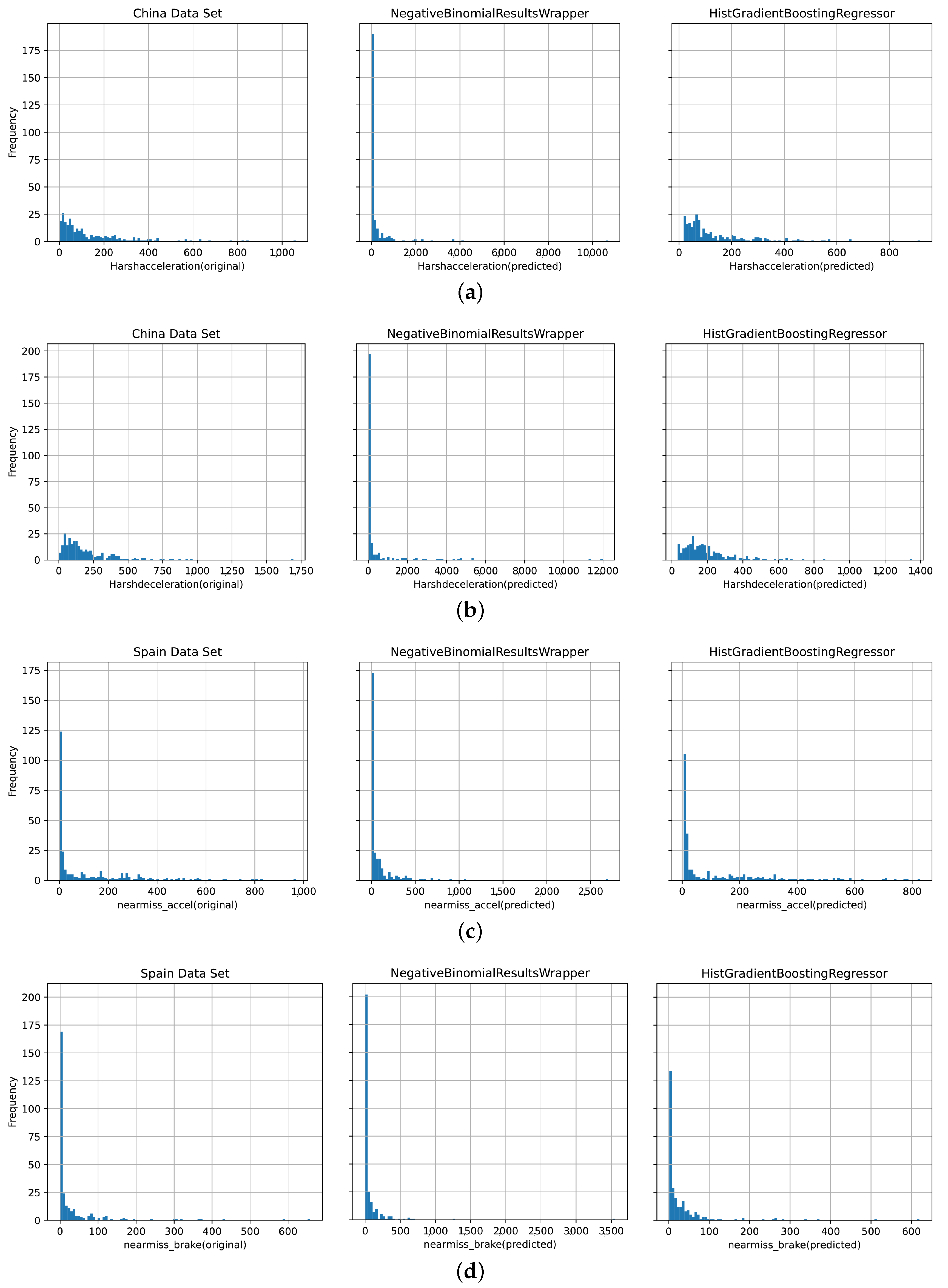
As illustrated in Figure 3, the HGBR exhibits superior predictive capabilities and more accurately simulates the data distribution of the two types of near-miss events in comparison to the negative binomial model across both datasets (from China and Spain). It has been observed that the negative binomial model’s predictions for zero values sometimes do not align with reality, unlike the HGBR, which demonstrates a good fit to actual data. This discrepancy may be attributed to the failure of the GLM to account for non-linear relationships among variables. There is also the fact that the prediction process of the GLM is actually an approximation to a hypothetical distribution, and once the actual situation is not a standard distribution, its predictive power is weakened. In contrast, the HGBR’s strength lies in its capacity to incorporate diverse data types and variable dependencies, which contributes to its exceptional predictive power.

Figure 3. Cumulative frequency comparison of the original value (left), negative binomial regression model predicted value (middle), HGBR model predicted value (right) on (a) Harshacceleration from the dataset from China, (b) Harshdeceleration from the dataset from China, (c) nearmiss_accel from the dataset from Spain, and (d) nearmiss_brake from the dataset from Spain.

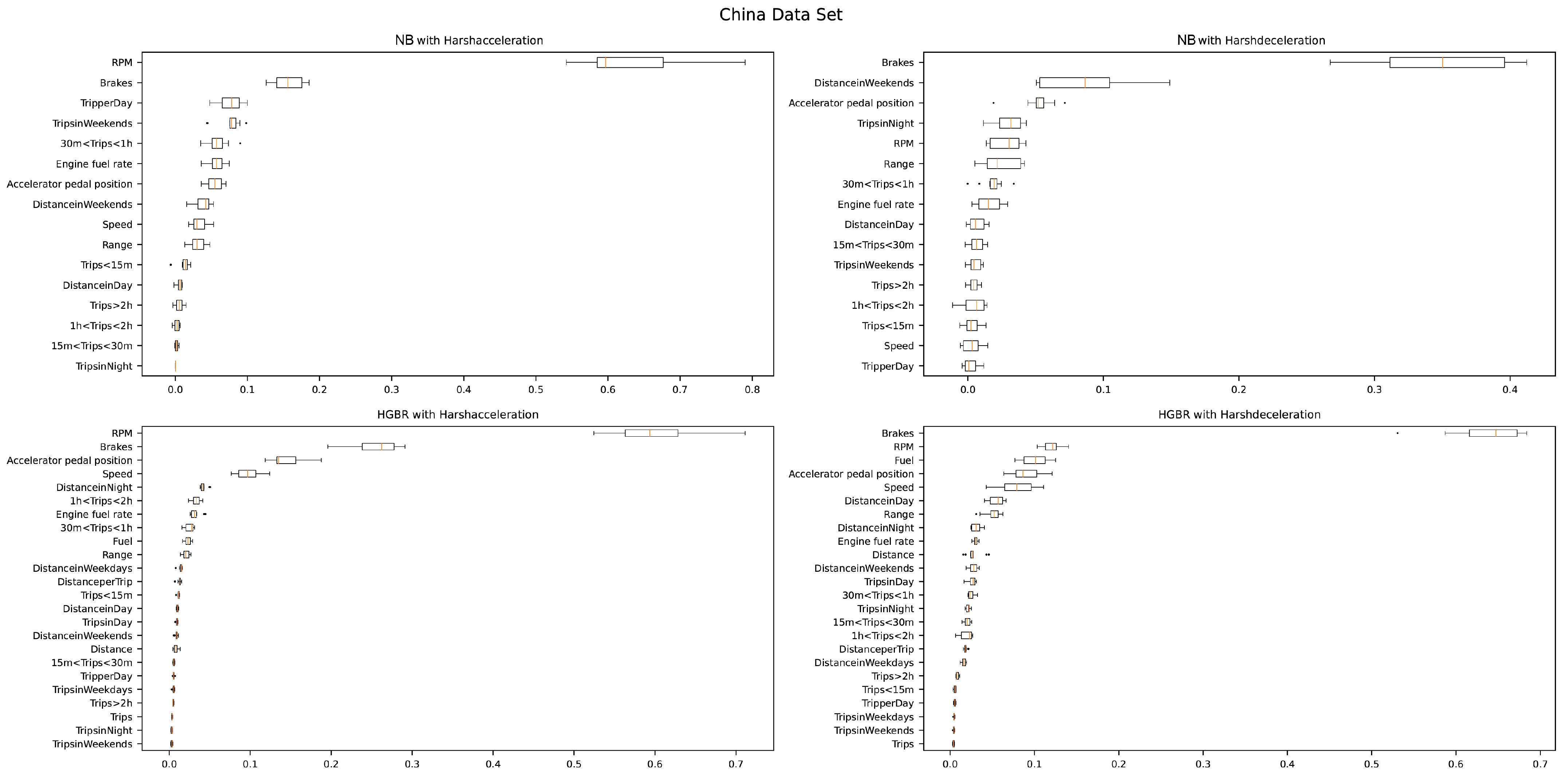
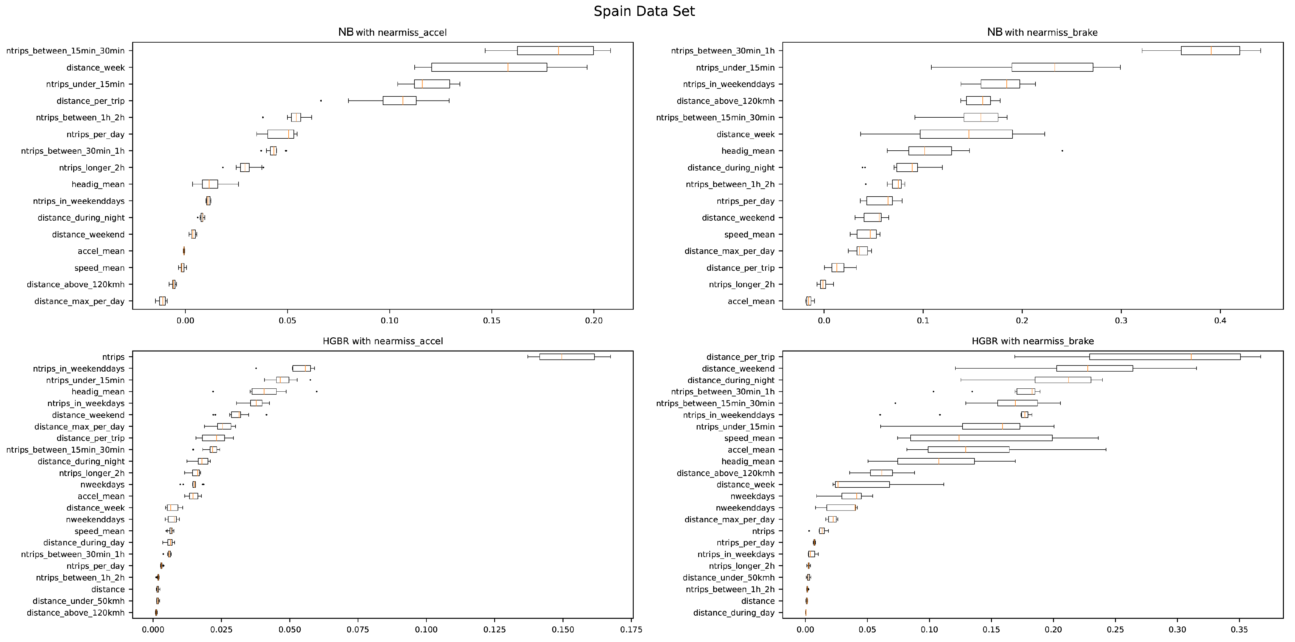
Permuted feature importance, one of the explanation tools of machine learning, could be derived from changes in model prediction errors following the disruption of eigenvalues [35]. To understand the contribution of features to model prediction, permuted feature importance tests are performed on the Poisson regression model and HGBR model, respectively. It can be seen from Figure 4 that the two models of the two near-miss event labels in the dataset from China are more sensitive to driving behavior variables. The same is true for the dataset from Spain, except that the model from the dataset from Spain is more sensitive to distance and duration variables, as shown in Figure 5. However, the characteristics of the same model do not contribute to the prediction of different labels. Due to the different features selected among different models, the comparison of feature contributions is meaningless. It is worth mentioning that the permuted feature importance of the negative binomial regression model is partially consistent with the variable significance shown in Table 7 and Table 8, but there are also contradictions. This means that this method can only be used as an aid to understanding the contribution of variables, and its reliability and interpretability need to be improved.

Figure 4. Feature importance ranking for the dataset from China; the upper left subgraph presents the results of negative binomial regression on Harshacceleration, the upper right subgraph presents the results of negative binomial regression on Harshdeceleration, the lower left subgraph presents the results of HGBR on Harshacceleration, and the lower right subgraph presents the results of HGBR on Harshdeceleration.

Figure 5. Feature importance ranking for the dataset from Spain; the upper left subgraph presents the results of negative binomial regression on nearmiss_accel, the upper right subgraph presents the results of negative binomial regression on nearmiss_brake, the lower left subgraph presents the results of HGBR on nearmiss_accel, and the lower right subgraph presents the results of HGBR on nearmiss_brake.

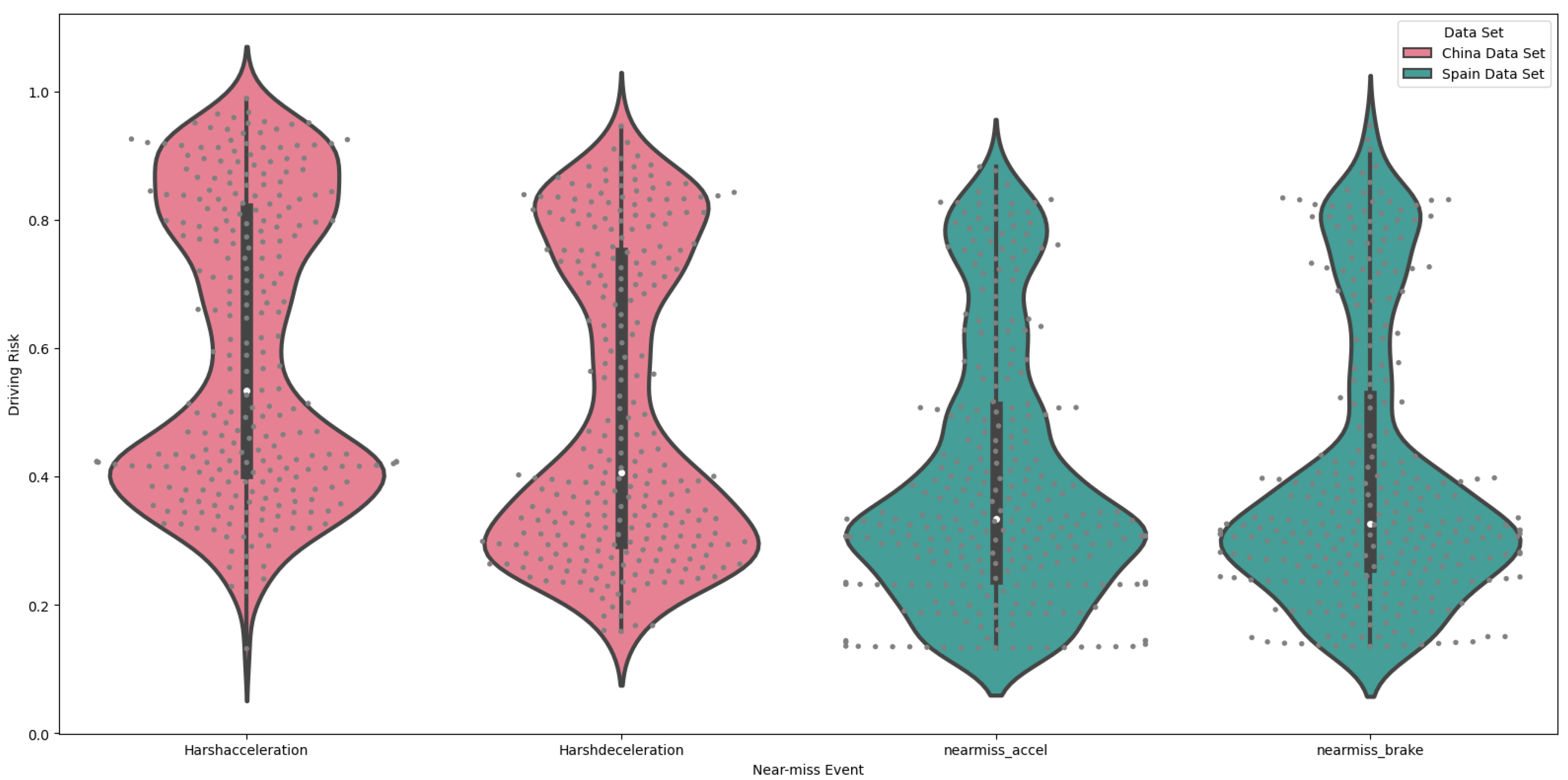
Once the aforementioned risk factor calculation method was employed to derive driving risks, the predicted outcomes from the HGBR were combined with the actual values of near-miss events from the two datasets. This process yielded four groups of driving risk factors, as detailed in Table 10. Due to the limited number of drivers, all these metrics were derived from the full sample. The distribution maps in Figure 6 illustrate the distribution of driving risks for each near-miss event. In each group, a point represents an observation’s driving risk factor, while the shaded areas and box plots represent the kernel density and distribution of observed driving risks. In the dataset from China, either in the $Harshacceleration$ group or in the $Harshdeceleration$ group, the driving risk for each near-miss event group is primarily concentrated into two clusters. The first cluster, comprising observations with a value above 0.6, indicates a high-risk group, while the second cluster, comprising observations with a value below 0.6, indicates a low-risk group. In the dataset from Spain, both the $near\_miss$ acceleration and $near\_miss$ braking groups indicate that the majority of drivers’ risks are distributed approximately normally around 0.3, whereas a minority are distributed approximately normally around 0.8.

Table 10. Driving risk factor description of different near-miss events on different datasets.

Dataset	Near-Miss Event	Count	Mean	Standard Deviation	Minimum	25%	50%	75%	Maximum
Dataset from China	Harshacceleration	261	0.597	0.226	0.132	0.406	0.534	0.817	0.989
Dataset from China	Harshdeceleration	261	0.503	0.233	0.158	0.298	0.406	0.747	0.946
Dataset from Spain	nearmiss_accel	285	0.400	0.205	0.133	0.241	0.333	0.507	0.883
Dataset from Spain	nearmiss_brake	285	0.406	0.217	0.135	0.259	0.326	0.524	0.947

Figure 6. Driving risk distribution for the dataset from China, which shows the Harshacceleration group (first pink on the left) and Harshdeceleration group (second pink on the left), and the dataset from Spain, which shows the nearmiss_accel group (first green on the right) and nearmiss_brake group (second green on the right).

While there is no inherent correlation between the four sets of driving risk factor outcomes, they do exhibit certain similarities. These include the magnitude of individual driving risks and how they are aggregated. The results demonstrate that—regardless of the dimension used to assess a driver’s risk-taking behavior—two distinct groups emerge: one with lower driving risk and another with higher driving risk. These groups exhibit a clear divergence, with the majority of ambiguous drivers occupying a relatively minor position. In general, the lower-risk drivers constitute the majority, yet it is not implausible that the majority of drivers may engage in more aggressive driving under certain circumstances. This result also proves that the driving risk scoring algorithm proposed in this study can effectively distinguish the driving risk levels. In addition, although laws and regulations in Spain differ from those in China, and neither auto insurance market currently offers a near-miss-based premium calculation product, this method demonstrates a straightforward way to show that near-miss events can be used as corrections to the price of subsequent periods. Furthermore, the same approach can be applied across different countries.

5. Conclusions

Near-miss events have been shown to be effective for assessing driving risks. Most independent variables in the GLM model are statistically significant, indicating that the model effectively captures the distribution pattern of near-miss events as dependent variables. The HGBR model demonstrates exemplary predictive capacity, ensuring accurate output variables derived from input variables. The values and distribution of driving risk factors align with prevailing expectations and understanding. This study’s findings suggest that near-miss events have the potential to serve as independent variables, providing valuable information for driving risk regression analysis. Furthermore, near-miss events may be utilized as substitutes for accidents or claims when scoring driving risks [36]. Additionally, driving risks can be leveraged to adjust premiums. However, the actuarial implications of such adjustments for insurance companies require analysis. In particular, issues such as the equilibrium of premiums and the distribution of payouts remain beyond the scope of this paper and necessitate further examination.

The aforementioned study raises an intriguing question about the potential benefits of employing driving risk predictors instead of directly using near-miss frequencies. We contend that predictive models offer an effective methodology for generating a risk score that incorporates contextual data beyond near-miss information. This data can be influenced by external factors unrelated to the driver, such as the hazardous actions of other drivers. Consequently, the risk score or predictive value provides a more accurate approximation of the expected number of near-miss events and, ultimately, the projected number of accidents.

Both conventional generalized linear models and machine learning algorithms have their own respective merits and limitations. The outcomes of Poisson regression and negative binomial regression indicate the effect size and statistical significance of each independent variable on the dependent variable. They also highlight the causal impact of telematics attributes on near-miss events. The high accuracy of the HGBR in predicting near-miss events demonstrates its robust capability in handling telematics data with multiple driving-related variables. In the context of applying driving risk to rate-making, the interpretability of the calculation method is highly valuable to policyholders. Meanwhile, the efficiency and precision of the algorithm enable insurers to process large volumes of driver data in an effective and precise manner.

It needs to be recognized that the findings of this study are constrained by a number of limitations pertaining to the availability of relevant data. Firstly, the dataset from China covers a duration of less than seven days, which precludes essential analyses such as comparisons between weekdays and weekends. This limited timeframe may not accurately represent annual driving behavior, particularly as it may be influenced by seasonal variations. Additionally, the restricted temporal range could contribute to inconsistencies in the reported significance of variables. Moreover, the dataset from Spain is insufficiently comprehensive, and the types and number of variables included are not as large as those in the dataset from China, which renders the results less interpretable. Furthermore, the lack of traditional insurance data and driving condition data represents a substantial limitation. Including factors that capture the characteristics of drivers is crucial for providing a comprehensive evaluation of the risks associated with driving.

Given the good performance of the ensemble learning algorithms used in this study, future research will explore the use of more interpretable machine learning algorithms for modeling and predicting large amounts of telematics data, and for car insurance pricing. While artificial neural networks are not inherently interpretable, they can nonetheless be explained using secondary tools or methods [37,38]. Thus, future research will explore how state-of-the-art artificial neural networks can be applied to auto insurance to change the persistent perception among insurers and administrators that such algorithms are completely black-box systems. Exploring and analyzing telematics data using AI methods is important for shifting our perceptions and decision-making processes from non-autonomous to semi-autonomous to fully autonomous driving.