Predictive Models for the Binary Diffusion Coefficient at Infinite Dilution in Polar and Nonpolar Fluids


Abstract
1. Introduction
2. Theory and Methods
2.1. Database Compilation
2.2. Variable Selection and Hyper-Parameter Optimization
2.3. Machine Learning Algorithms
2.4. Classic Models
3. Results and Discussion
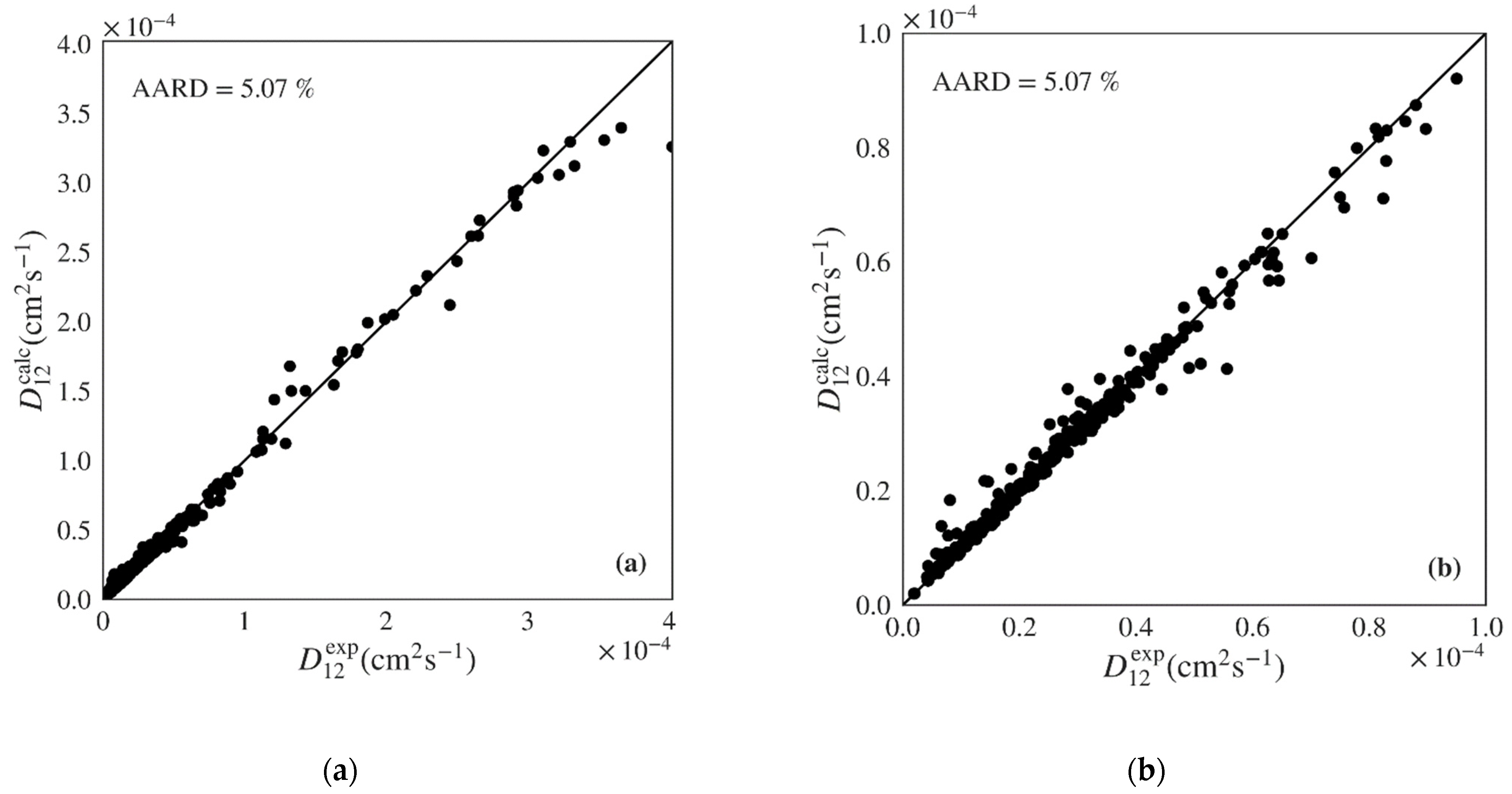
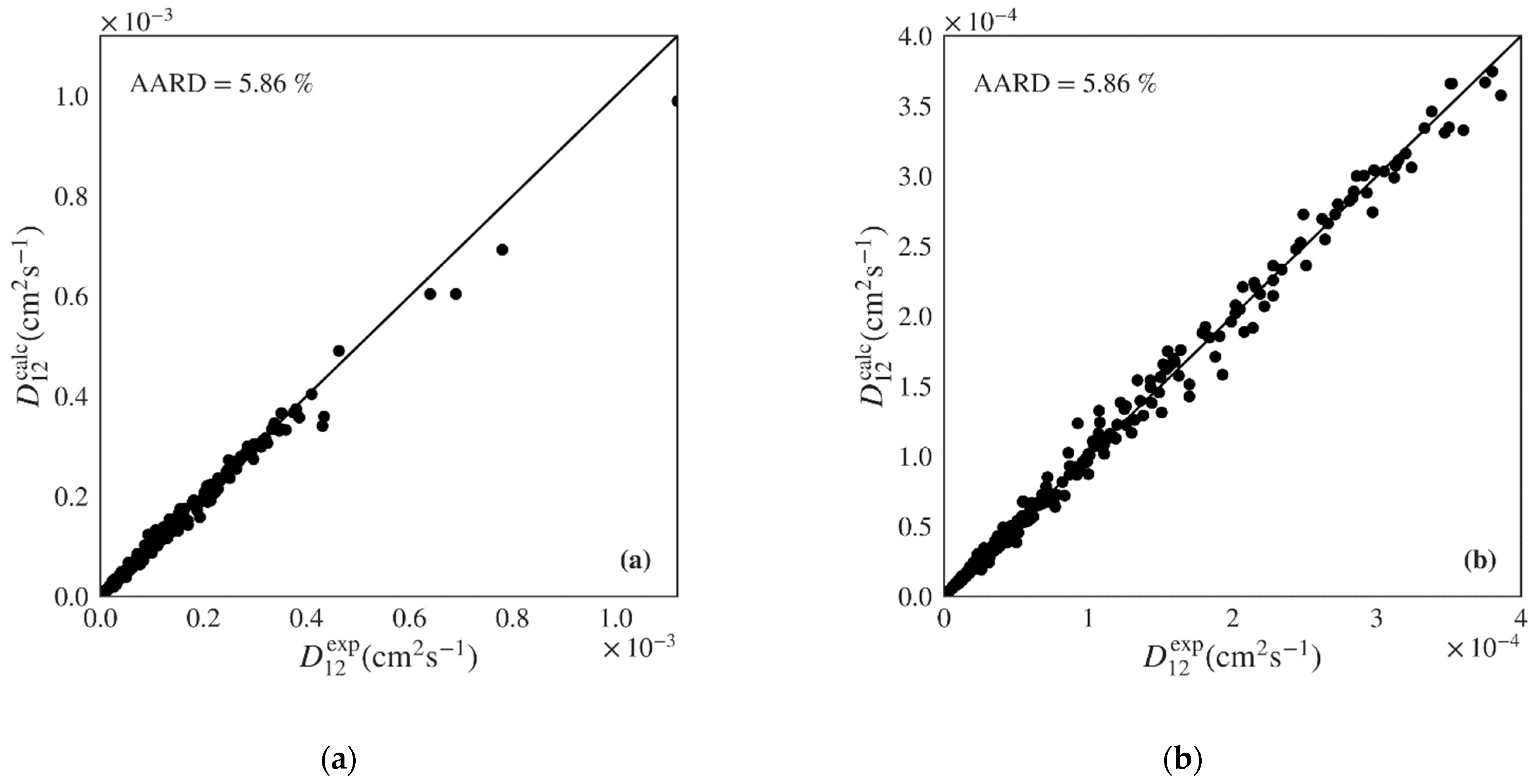
3.1. Machine Learning Models
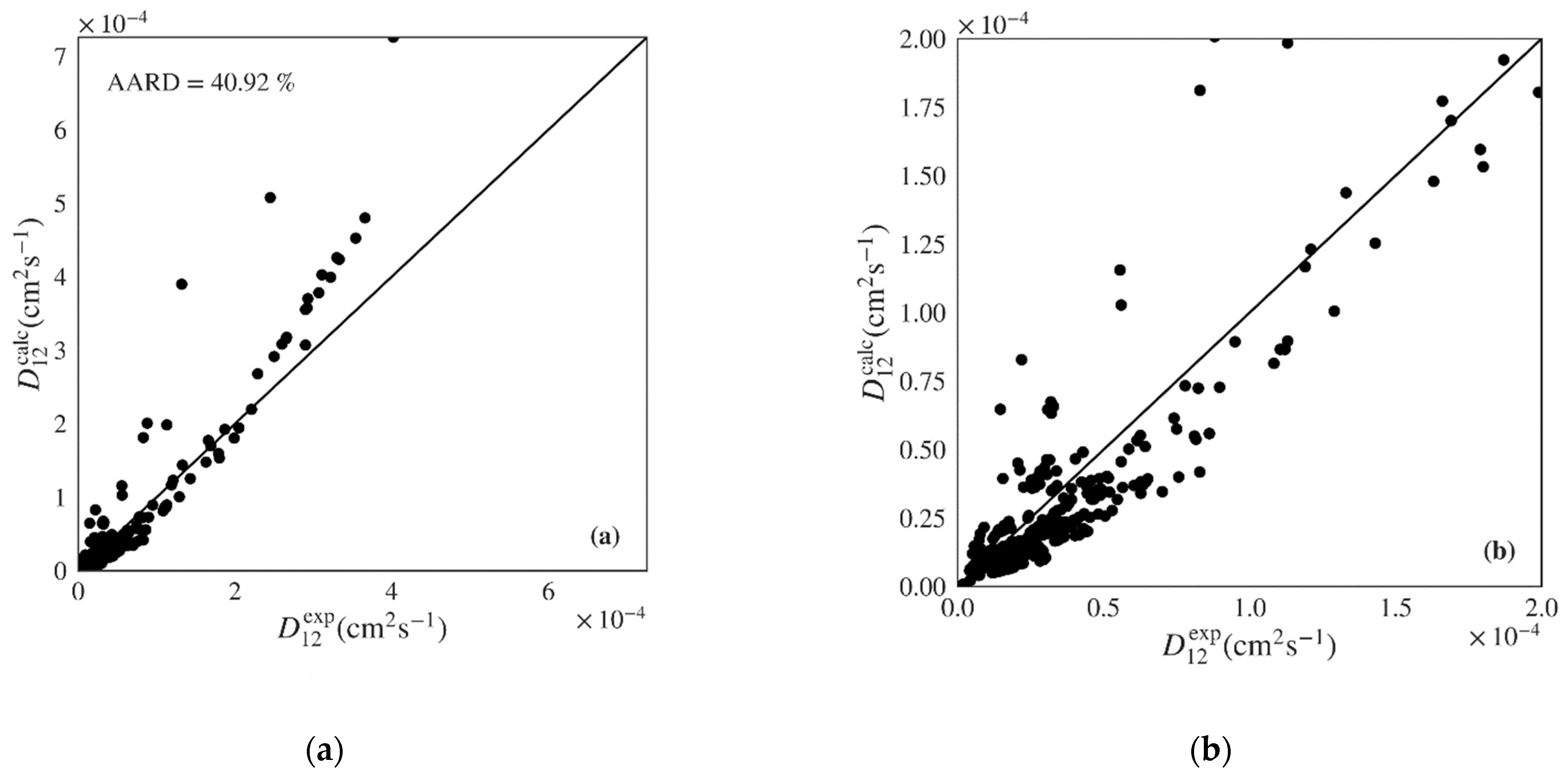
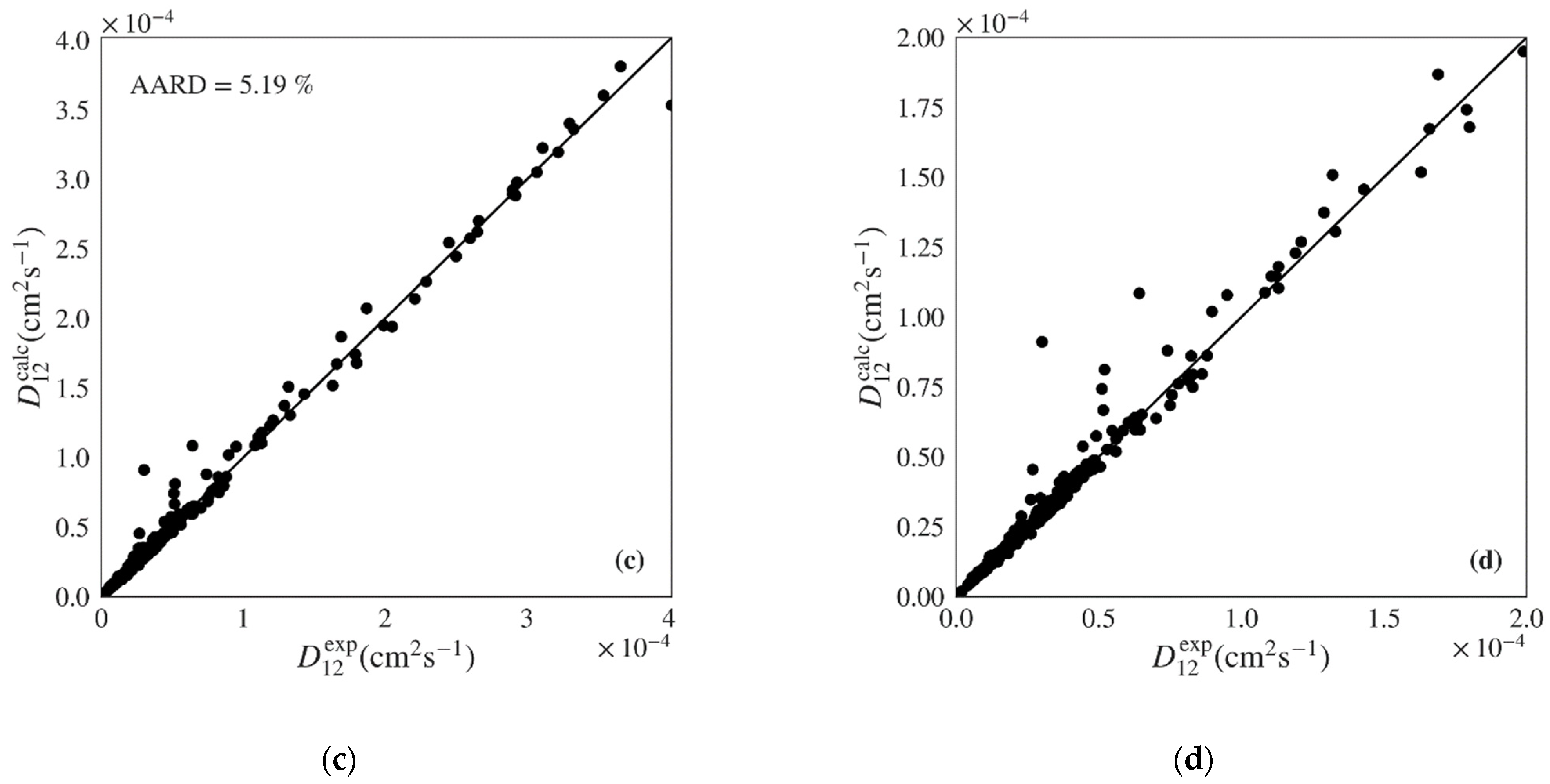
3.2. Detailed Comparison of ML Gradient Boosted and Classic Models
4. Conclusions
Supplementary Materials
Author Contributions
Funding
Institutional Review Board Statement
Informed Consent Statement
Data Availability Statement
Conflicts of Interest
References
- Wankat, P.C. Rate-Controlled Separations; Blackie Academic & Professional: Glasgow, UK, 1994. [Google Scholar]
- Oliveira, E.L.G.; Silvestre, A.J.D.; Silva, C.M. Review of kinetic models for supercritical fluid extraction. Chem. Eng. Res. Des. 2011, 89, 1104–1117. [Google Scholar] [CrossRef]
- Carberry, J.J. Chemical and Catalytic Reaction Engineering; McGraw-Hill: New York, NY, USA, 1971. [Google Scholar]
- Zêzere, B.; Portugal, I.; Gomes, J.R.B.; Silva, C.M. Revisiting Tracer Liu-Silva-Macedo model for binary diffusion coefficient using the largest database of liquid and supercritical systems. J. Supercrit. Fluids 2021, 168, 105073. [Google Scholar] [CrossRef]
- Wilke, C.R.; Chang, P. Correlation of diffusion coefficients in dilute solutions. AIChE J. 1955, 1, 264–270. [Google Scholar] [CrossRef]
- Scheibel, E.G. Liquid Diffusivities. Ind. Eng. Chem. 1954, 9, 2007–2008. [Google Scholar] [CrossRef]
- Tyn, M.T.; Calus, W.F. Diffusion Coefficients in Dilute Binary Liquid Mixtures. J. Chem. Eng. Data 1975, 20, 106–109. [Google Scholar] [CrossRef]
- Hayduk, W.; Minhas, B.S. Correlations for prediction of molecular diffusivities in liquids. Can. J. Chem. Eng. 1982, 60, 295–299. [Google Scholar] [CrossRef]
- Magalhães, A.L.; Lito, P.F.; Da Silva, F.A.; Silva, C.M. Simple and accurate correlations for diffusion coefficients of solutes in liquids and supercritical fluids over wide ranges of temperature and density. J. Supercrit. Fluids 2013, 76, 94–114. [Google Scholar] [CrossRef]
- Magalhães, A.L.; Da Silva, F.A.; Silva, C.M. Tracer diffusion coefficients of polar systems. Chem. Eng. Sci. 2012, 73, 151–168. [Google Scholar] [CrossRef]
- Dymond, J.H. Corrected Enskog theory and the transport coefficients of liquids. J. Chem. Phys. 1974, 60, 969–973. [Google Scholar] [CrossRef]
- Silva, C.M.; Liu, H. Modelling of Transport Properties of Hard Sphere Fluids and Related Systems, and its Applications. In Theory and Simulation of Hard-Sphere Fluids and Related Systems; Springer: Berlin, Germany, 2008; pp. 383–492. [Google Scholar]
- Zhu, Y.; Lu, X.; Zhou, J.; Wang, Y.; Shi, J. Prediction of diffusion coefficients for gas, liquid and supercritical fluid: Application to pure real fluids and infinite dilute binary solutions based on the simulation of Lennard–Jones fluid. Fluid Phase Equilib. 2002, 194–197, 1141–1159. [Google Scholar] [CrossRef]
- Magalhães, A.L.; Cardoso, S.P.; Figueiredo, B.R.; Da Silva, F.A.; Silva, C.M. Revisiting the liu-silva-macedo model for tracer diffusion coefficients of supercritical, liquid, and gaseous systems. Ind. Eng. Chem. Res. 2010, 49, 7697–7700. [Google Scholar] [CrossRef]
- Liu, H.; Silva, C.M.; Macedo, E.A. New Equations for Tracer Diffusion Coefficients of Solutes in Supercritical and Liquid Solvents Based on the Lennard-Jones Fluid Model. Ind. Eng. Chem. Res. 1997, 36, 246–252. [Google Scholar] [CrossRef]
- Gharagheizi, F.; Sattari, M. Estimation of molecular diffusivity of pure chemicals in water: A quantitative structure-property relationship study. SAR QSAR Environ. Res. 2009, 20, 267–285. [Google Scholar] [CrossRef] [PubMed]
- Khajeh, A.; Rasaei, M.R. Diffusion coefficient prediction of acids in water at infinite dilution by QSPR method. Struct. Chem. 2011, 23, 399–406. [Google Scholar] [CrossRef]
- Beigzadeh, R.; Rahimi, M.; Shabanian, S.R. Developing a feed forward neural network multilayer model for prediction of binary diffusion coefficient in liquids. Fluid Phase Equilib. 2012, 331, 48–57. [Google Scholar] [CrossRef]
- Eslamloueyan, R.; Khademi, M.H. A neural network-based method for estimation of binary gas diffusivity. Chemom. Intell. Lab. Syst. 2010, 104, 195–204. [Google Scholar] [CrossRef]
- Abbasi, A.; Eslamloueyan, R. Determination of binary diffusion coefficients of hydrocarbon mixtures using MLP and ANFIS networks based on QSPR method. Chemom. Intell. Lab. Syst. 2014, 132, 39–51. [Google Scholar] [CrossRef]
- Mirkhani, S.A.; Gharagheizi, F.; Sattari, M. A QSPR model for prediction of diffusion coefficient of non-electrolyte organic compounds in air at ambient condition. Chemosphere 2012, 86, 959–966. [Google Scholar] [CrossRef]
- Rahimi, M.R.; Karimi, H.; Yousefi, F. Prediction of carbon dioxide diffusivity in biodegradable polymers using diffusion neural network. Heat Mass Transf. Stoffuebertragung 2012, 48, 1357–1365. [Google Scholar] [CrossRef]
- Lashkarbolooki, M.; Hezave, A.Z.; Bayat, M. Thermal diffusivity of hydrocarbons and aromatics: Artificial neural network predicting model. J. Thermophys. Heat Transf. 2017, 31, 621–627. [Google Scholar] [CrossRef]
- Chudzik, S. Measurement of thermal diffusivity of insulating material using an artificial neural network. Meas. Sci. Technol. 2012, 23, 065602. [Google Scholar] [CrossRef]
- Aniceto, J.P.S.; Zêzere, B.; Silva, C.M. Machine learning models for the prediction of diffusivities in supercritical CO2 systems. J. Mol. Liq. 2021, 115281. [Google Scholar] [CrossRef]
- Yaws, C.L. Chemical Properties Handbook: Physical, Thermodynamic, Environmental, Transport, Safety, and Health Related Properties for Organic and Inorganic Chemicals; McGraw-Hill Professional: New York, NY, USA, 1998. [Google Scholar]
- Cibulka, I.; Ziková, M. Liquid densities at elevated pressures of 1-alkanols from C1 to C10: A critical evaluation of experimental data. J. Chem. Eng. Data 1994, 39, 876–886. [Google Scholar] [CrossRef]
- Cibulka, I.; Hnědkovský, L.; Takagi, T. P−$ρ$−T data of liquids: Summarization and evaluation. 4. Higher 1-alkanols (C11, C12, C14, C16), secondary, tertiary, and branched alkanols, cycloalkanols, alkanediols, alkanetriols, ether alkanols, and aromatic hydroxy derivatives. J. Chem. Eng. Data 1997, 42, 415–433. [Google Scholar] [CrossRef]
- Cibulka, I.; Takagi, T.; Růžička, K. P−ρ−T data of liquids: Summarization and evaluation. 7. Selected halogenated hydrocarbons. J. Chem. Eng. Data 2000, 46, 2–28. [Google Scholar] [CrossRef]
- Cibulka, I.; Takagi, T. P−ρ−T data of liquids: Summarization and evaluation. 8. Miscellaneous compounds. J. Chem. Eng. Data 2002, 47, 1037–1070. [Google Scholar] [CrossRef]
- Reid, R.C.; Prausnitz, J.M.; Poling, B.E. The Properties of Gases and Liquids, 4th ed.; Company, M.-H.B., Ed.; McGraw-Hill International Editions: New York, NY, USA, 1987. [Google Scholar]
- Viswanath, D.S.; Ghosh, T.K.; Prasad, D.H.; Dutt, N.V.K.; Rani, K.Y. Viscosity of Liquids: Theory, Estimation, Experiment, and Data; Springer: Dordrecht, The Netherlands, 2007; ISBN 978-1-4020-5482-2. [Google Scholar]
- Lucas, K. Ein einfaches verfahren zur berechnung der viskosität von Gasen und Gasgemischen. Chem. Ing. Tech. 1974, 46, 157–158. [Google Scholar] [CrossRef]
- Assael, M.J.; Dymond, J.H.; Polimatidou, S.K. Correlation and prediction of dense fluid transport coefficients. Fluid Phase Equilib. 1994, 15, 189–201. [Google Scholar] [CrossRef]
- Cano-Gómez, J.J.; Iglesias-Silva, G.A.; Rico-Ramírez, V.; Ramos-Estrada, M.; Hall, K.R. A new correlation for the prediction of refractive index and liquid densities of 1-alcohols. Fluid Phase Equilib. 2015, 387, 117–120. [Google Scholar] [CrossRef]
- Pádua, A.A.H.; Fareleira, J.M.N.A.; Calado, J.C.G.; Wakeham, W.A. Density and viscosity measurements of 2,2,4-trimethylpentane (isooctane) from 198 K to 348 K and up to 100 MPa. J. Chem. Eng. Data 1996, 41, 1488–1494. [Google Scholar] [CrossRef]
- Tyn, M.T.; Calus, W.F. Estimating liquid molar volume. Processing 1975, 21, 16–17. [Google Scholar]
- ChemSpider—Building Community for Chemists. Available online: http://www.chemspider.com (accessed on 22 August 2020).
- Korea Thermophysical Properties Data Bank (KDB). Available online: http://www.cheric.org/research/kdb/hcprop/cmpsrch.php (accessed on 22 August 2020).
- Design Institute for Physical Properties (DIPPR). Available online: http://dippr.byu.edu/ (accessed on 22 August 2020).
- Yaws, C.L. Thermophysical Properties of Chemicals and Hydrocarbons; William Andrew Inc.: New York, NY, USA, 2008. [Google Scholar]
- LookChem.com—Look for Chemicals. Available online: http://www.lookchem.com (accessed on 22 August 2020).
- AspenTech. Aspen Physical Property System—Physical Property Methods; AspenTech: Cambridge, MA, USA, 2007. [Google Scholar]
- Cordeiro, J. Medição e Modelação de Difusividades em CO2 Supercrítico e Etanol; Universidade de Aveiro: Aveiro, Potugal, 2015. [Google Scholar]
- Joback, K.G.; Reid, R.C. A Unified Approach to physical Property Estimation Using Multivariate Statistical Techniques; Massachusetts Institute of Technology: Cambridge, MA, USA, 1984. [Google Scholar]
- Joback, K.G.; Reid, R.C. Estimation of pure-component properties from group-contributions. Chem. Eng. Commun. 1987, 57, 233–243. [Google Scholar] [CrossRef]
- Somayajulu, G.R. Estimation Procedures for Critical Constants. J. Chem. Eng. Data 1989, 34, 106–120. [Google Scholar] [CrossRef]
- Klincewicz, K.M.; Reid, R.C. Estimation of critical properties with group contribution methods. AIChE J. 1984, 30, 137–142. [Google Scholar] [CrossRef]
- Ambrose, D. Correlation and estimation of vapour-liquid critical properties. I: Critical temperatures of organic compounds. In NPL Technical Report Chem. 92; National Physical Lab.: London, UK, 1978. [Google Scholar]
- Ambrose, D. Correlation and Estimation of Vapour-Liquid Critical Properties. II: Critical Pressure and Critical Volume. In NPL Technical Report. Chem. 92; National Physical Lab.: London, UK, 1979. [Google Scholar]
- Green, D.W.; Perry, R.H. Perry’s Chemical Engineers’ Handbook, 8th ed.; McGraw-Hill Professional: New York, NY, USA, 2008. [Google Scholar]
- Wen, X.; Qiang, Y. A new group contribution method for estimating critical properties of organic compounds. Ind. Eng. Chem. Res. 2001, 40, 6245–6250. [Google Scholar] [CrossRef]
- Valderrama, J.O.; Rojas, R.E. Critical properties of ionic liquids. Revisited. Ind. Eng. Chem. Res. 2009, 48, 6890–6900. [Google Scholar] [CrossRef]
- Lee, B.I.; Kesler, M.G. A generalized thermodynamic correlation based on three-parameter corresponding states. AIChE J. 1975, 21, 510–527. [Google Scholar] [CrossRef]
- Pitzer, K.S.; Lippmann, D.Z.; Curl, R.F.; Huggins, C.M.; Petersen, D.E. The Volumetric and Thermodynamic Properties of Fluids. II. Compressibility Factor, Vapor Pressure and Entropy of Vaporization. J. Am. Chem. Soc. 1955, 77, 3433–3440. [Google Scholar] [CrossRef]
- Zêzere, B.; Magalhães, A.L.; Portugal, I.; Silva, C.M. Diffusion coefficients of eucalyptol at infinite dilution in compressed liquid ethanol and in supercritical CO2/ethanol mixtures. J. Supercrit. Fluids 2018, 133, 297–308. [Google Scholar] [CrossRef]
- Leite, J.; Magalhães, A.L.; Valente, A.A.; Silva, C.M. Measurement and modelling of tracer diffusivities of gallic acid in liquid ethanol and in supercritical CO2 modified with ethanol. J. Supercrit. Fluids 2018, 131, 130–139. [Google Scholar] [CrossRef]
- Catchpole, O.J.; Von Kamp, J.C. Phase equilibrium for the extraction of squalene from shark liver oil using supercritical carbon dioxide. Ind. Eng. Chem. Res. 1997, 36, 3762–3768. [Google Scholar] [CrossRef]
- Liu, H.; Silva, C.M.; Macedo, E.A. Unified approach to the self-diffusion coefficients of dense fluids over wide ranges of temperature and pressure-hard-sphere, square-well, Lennard-Jones and real substances. Chem. Eng. Sci. 1998, 53, 2403–2422. [Google Scholar] [CrossRef]
- Cordeiro, J.; Magalhães, A.L.; Valente, A.A.; Silva, C.M. Experimental and theoretical analysis of the diffusion behavior of chromium(III) acetylacetonate in supercritical CO2. J. Supercrit. Fluids 2016, 118, 153–162. [Google Scholar] [CrossRef]
- Burkov, A. The Hundred-Page Machine Learning Book; Andriy Burkov: Quebec City, QC, Canada, 2019; ISBN 978-1-99-957950-0. [Google Scholar]
- Pedregosa, F.; Varoquaux, G.; Gramfort, A.; Michel, V.; Thirion, B.; Grisel, O.; Blondel, M.; Prettenhofer, P.; Weiss, R.; Dubourg, V.; et al. Scikit-learn: Machine learning in Python. J. Mach. Learn. Res. 2011, 12, 2825–2830. [Google Scholar]
- Hastie, T.; Tibshirani, R.; Friedman, J. The Elements of Statistical Learning, 2nd ed.; Springer: New York, NY, USA, 2009; ISBN 978-0-38-784857-0. [Google Scholar]
- Altman, N.S. An introduction to kernel and nearest-neighbor nonparametric regression. Am. Stat. 1992, 46, 175–185. [Google Scholar] [CrossRef]
- Mitchell, J.B.O. Machine learning methods in chemoinformatics. Wiley Interdiscip. Rev. Comput. Mol. Sci. 2014, 4, 468–481. [Google Scholar] [CrossRef]
- Quinlan, J.R. Simplifying decision trees. Int. J. Man. Mach. Stud. 1987, 27, 221–234. [Google Scholar] [CrossRef]
- Müller, A.C.; Guido, S. Introduction to Machine Learning with Python: A Guide for Data Scientists; O’Reilly Media, Inc.: Sebastopol, CA, USA, 2016; ISBN 978-1-449-36941-5. [Google Scholar]
- Breiman, L. Random forests. Mach. Learn. 2001, 45, 5–32. [Google Scholar] [CrossRef]
- Friedman, J.H. Greedy function approximation: A gradient boosting machine. Ann. Stat. 2001, 29, 1189–1232. [Google Scholar] [CrossRef]
- Svetnik, V.; Wang, T.; Tong, C.; Liaw, A.; Sheridan, R.P.; Song, Q. Boosting: An ensemble learning tool for compound classification and QSAR modeling. J. Chem. Inf. Model. 2005, 45, 786–799. [Google Scholar] [CrossRef]
- Cooper, E. Diffusion Coefficients at Infinite Dilution in Alcohol Solvents at Temperatures to 348 K and Pressures to 17 MPa; University of Ottawa: Ottawa, ON, Canada, 1992. [Google Scholar]
- Pratt, K.C.; Wakeham, W.A. The mutual diffusion coefficient for binary mixtures of water and the isomers of propanol. Proc. R. Soc. Lond. A 1975, 342, 401–419. [Google Scholar] [CrossRef]
- Sun, C.K.J.; Chen, S.-H. Tracer diffusion in dense methanol and 2-propanol up to supercritical region: Understanding of solvent molecular association and development of an empirical correlation. Ind. Eng. Chem. Res. 1987, 24, 815–819. [Google Scholar] [CrossRef]
- Man, C.W. Limiting Mutual Diffusion of Nonassociated Aromatic Solutes; The Hong Kong Polytechnic University: Hong Kong, China, 2001. [Google Scholar]
- Tyn, M.T.; Calus, W.F. Temperature and concentration dependence of mutual diffusion coefficients of some binary liquid systems. J. Chem. Eng. Data 1975, 20, 310–316. [Google Scholar] [CrossRef]
- Sarraute, S.; Gomes, M.F.C.; Pádua, A.A.H. Diffusion coefficients of 1-alkyl-3-methylimidazolium ionic liquids in water, methanol, and acetonitrile at infinite dilution. J. Chem. Eng. Data 2009, 54, 2389–2394. [Google Scholar] [CrossRef]
- Hurle, R.L.; Woolf, L.A. Tracer diffusion in methanol and acetonitrile under pressure. J. Chem. Soc. Faraday Trans. 1982, 78, 2921–2928. [Google Scholar] [CrossRef]
- Wong, C.-F.; Hayduk, W. Molecular diffusivities for propene in 1-butanol, chlorobenzene, ethylene glycol, and n-octane at elevated pressures. J. Chem. Eng. Data 1990, 35, 323–328. [Google Scholar] [CrossRef]
- Wong, C.-F. Diffusion Coefficients of Dissolved Gases in Liquids; University of Ottawa: Ottawa, ON, Canada, 1989. [Google Scholar]
- Kopner, A.; Hamm, A.; Ellert, J.; Feist, R.; Schneider, G.M. Determination of binary diffusion coefficients in supercritical chlorotrifluoromethane and sulfurhexafluoride with supercritical fluid chromatography (SFC). Chem. Eng. Sci. 1987, 42, 2213–2218. [Google Scholar] [CrossRef]
- Han, P.; Bartels, D.M. Temperature dependence of oxygen diffusion in H2O and D2O. J. Phys. Chem. 1996, 100, 5597–5602. [Google Scholar] [CrossRef]
- Tominaga, T.; Matsumoto, S. Diffusion of polar and nonpolar molecules in water and ethanol. Bull. Chem. Soc. Jpn. 1990, 63, 533–537. [Google Scholar] [CrossRef]
- Sun, C.K.J.; Chen, S.H. Tracer diffusion in dense ethanol: A generalized correlation for nonpolar and hydrogen-bonded solvents. AIChE J. 1986, 32, 1367–1371. [Google Scholar] [CrossRef]
- Suárez-Iglesias, O.; Medina, I.; Pizarro, C.; Bueno, J.L. Diffusion of benzyl acetate, 2-phenylethyl acetate, 3-phenylpropyl acetate, and dibenzyl ether in mixtures of carbon dioxide and ethanol. Ind. Eng. Chem. Res. 2007, 46, 3810–3819. [Google Scholar] [CrossRef]
- Lin, I.-H.; Tan, C.-S. Diffusion of benzonitrile in CO2—Expanded ethanol. J. Chem. Eng. Data 2008, 53, 1886–1891. [Google Scholar] [CrossRef]
- Kong, C.Y.; Watanabe, K.; Funazukuri, T. Measurement and correlation of the diffusion coefficients of chromium(III) acetylacetonate at infinite dilution in supercritical carbon dioxide and in liquid ethanol. J. Chem. Thermodyn. 2017, 105, 86–93. [Google Scholar] [CrossRef]
- Zêzere, B.; Cordeiro, J.; Leite, J.; Magalhães, A.L.; Portugal, I.; Silva, C.M. Diffusivities of metal acetylacetonates in liquid ethanol and comparison with the transport behavior in supercritical systems. J. Supercrit. Fluids 2019, 143, 259–267. [Google Scholar] [CrossRef]
- Funazukuri, T.; Yamasaki, T.; Taguchi, M.; Kong, C.Y. Measurement of binary diffusion coefficient and solubility estimation for dyes in supercritical carbon dioxide by CIR method. Fluid Phase Equilib. 2015, 420, 7–13. [Google Scholar] [CrossRef]
- Kong, C.Y.; Sugiura, K.; Natsume, S.; Sakabe, J.; Funazukuri, T.; Miyake, K.; Okajima, I.; Badhulika, S.; Sako, T. Measurements and correlation of diffusion coefficients of ibuprofen in both liquid and supercritical fluids. J. Supercrit. Fluids 2020, 159, 104776. [Google Scholar] [CrossRef]
- Snijder, E.D.; te Riele, M.J.M.; Versteeg, G.F.; van Swaaij, W.P.M. Diffusion Coefficients of CO, CO2, N2O, and N2 in ethanol and toluene. J. Chem. Eng. Data 1995, 40, 37–39. [Google Scholar] [CrossRef]
- Kong, C.Y.; Watanabe, K.; Funazukuri, T. Diffusion coefficients of phenylbutazone in supercritical CO2 and in ethanol. J. Chromatogr. A 2013, 1279, 92–97. [Google Scholar] [CrossRef]
- Zêzere, B.; Iglésias, J.; Portugal, I.; Gomes, J.R.B.; Silva, C.M. Diffusion of quercetin in compressed liquid ethyl acetate and ethanol. J. Mol. Liq. 2020, 114714. [Google Scholar] [CrossRef]
- Pratt, K.C.; Wakeham, W.A. The mutual diffusion coefficient of ethanol-water mixtures: Determination by a rapid, new method. Proc. R. Soc. Lond. A 1974, 336, 393–406. [Google Scholar]
- Zêzere, B.; Silva, J.M.; Portugal, I.; Gomes, J.R.B.; Silva, C.M. Measurement of astaxanthin and squalene diffusivities in compressed liquid ethyl acetate by Taylor-Aris dispersion method. Sep. Purif. Technol. 2020, 234, 116046. [Google Scholar] [CrossRef]
- Heintz, A.; Ludwig, R.; Schmidt, E. Limiting diffusion coefficients of ionic liquids in water and methanol: A combined experimental and molecular dynamics study. Phys. Chem. Chem. Phys. 2011, 13, 3268–3273. [Google Scholar] [CrossRef] [PubMed]
- Liu, Q.; Takemura, F.; Yabe, A. Solubility and diffusivity of carbon monoxide in liquid methanol. J. Chem. Eng. Data 1996, 41, 589–592. [Google Scholar] [CrossRef]
- Lin, I.-H.; Tan, C.-S. Measurement of diffusion coefficients of p-chloronitrobenzene in CO2-expanded methanol. J. Supercrit. Fluids 2008, 46, 112–117. [Google Scholar] [CrossRef]
- Funazukuri, T.; Sugihara, T.; Yui, K.; Ishii, T.; Taguchi, M. Measurement of infinite dilution diffusion coefficients of vitamin K3 in CO2 expanded methanol. J. Supercrit. Fluids 2016, 108, 19–25. [Google Scholar] [CrossRef]
- Lee, Y.E.; Li, F.Y. Binary diffusion coefficients of the methanol water system in the temperature range 30–40 °C. J. Chem. Eng. Data 1991, 36, 240–243. [Google Scholar] [CrossRef]
- Fan, Y.Q.; Qian, R.Y.; Shi, M.R.; Shi, J. Infinite dilution diffusion coefficients of several aromatic hydrocarbons in octane and 2,2,4-trimethylpentane. J. Chem. Eng. Data 1995, 40, 1053–1055. [Google Scholar] [CrossRef]
- Sun, C.K.J.; Chen, S.H. Diffusion of benzene, toluene, naphthalene, and phenanthrene in supercritical dense 2,3-dimethylbutane. AIChE J. 1985, 31, 1904–1910. [Google Scholar] [CrossRef]
- Toriurmi, M.; Katooka, R.; Yui, K.; Funazukuri, T.; Kong, C.Y.; Kagei, S. Measurements of binary diffusion coefficients for metal complexes in organic solvents by the Taylor dispersion method. Fluid Phase Equilib. 2010, 297, 62–66. [Google Scholar] [CrossRef]
- Sun, C.K.J.; Chen, S.H. Tracer diffusion of aromatic hydrocarbons in n-hexane up to the supercritical region. Chem. Eng. Sci. 1985, 40, 2217–2224. [Google Scholar]
- Funazukuri, T.; Nishimoton, N.; Wakao, N. Binary diffusion coefficients of organic compounds in hexane, dodecane, and cyclohexane at 303.2-333.2 K and 16.0 MPa. J. Chem. Eng. Data 1994, 39, 911–915. [Google Scholar] [CrossRef]
- Chen, S.H.; Davis, H.T.; Evans, D.F. Tracer diffusion in polyatomic liquids. II. J. Chem. Phys. 1981, 75, 1422–1426. [Google Scholar] [CrossRef]
- Sun, C.K.J.; Chen, S.H. Tracer diffusion of aromatic hydrocarbons in liquid cyclohexane up to its critical temperature. AIChE J. 1985, 31, 1510–1515. [Google Scholar] [CrossRef]
- Chen, B.H.C.; Sun, C.K.J.; Chen, S.H. Hard sphere treatment of binary diffusion in liquid at high dilution up to the critical temperature. J. Chem. Phys. 1985, 82, 2052–2055. [Google Scholar] [CrossRef]
- Noel, J.M.; Erkey, C.; Bukur, D.B.; Akgerman, A. Infinite dilution mutual diffusion coefficients of 1-octene and 1-tetradecene in near-critical ethane and propane. J. Chem. Eng. Data 1994, 39, 920–921. [Google Scholar] [CrossRef]
- Chen, H.C.; Chen, S.H. Tracer diffusion of crown ethers in n-decane and n-tetradecane: An improved correlation for binary systems involving normal alkanes. Ind. Eng. Chem. Fundam. 1985, 24, 187–192. [Google Scholar] [CrossRef]
- Chen, S.H.; Davis, H.T.; Evans, D.F. Tracer diffusion in polyatomic liquids. III. J. Chem. Phys. 1982, 77, 2540–2544. [Google Scholar] [CrossRef]
- Pollack, G.L.; Kennan, R.P.; Himm, J.F.; Stump, D.R. Diffusion of xenon in liquid alkanes: Temperature dependence measurements with a new method. Stokes–Einstein and hard sphere theories. J. Chem. Phys. 1990, 92, 625–630. [Google Scholar] [CrossRef]
- Matthews, M.A.; Rodden, J.B.; Akgerman, A. High-temperature diffusion of hydrogen, carbon monoxide, and carbon dioxide in liquid n-heptane, n-dodecane, and n-hexadecane. J. Chem. Eng. Data 1987, 32, 319–322. [Google Scholar] [CrossRef]
- Matthews, M.A.; Akgerman, A. Diffusion coefficients for binary alkane mixtures to 573 K and 3.5 MPa. AIChE J. 1987, 33, 881–885. [Google Scholar] [CrossRef]
- Rodden, J.B.; Erkey, C.; Akgerman, A. High-temperature diffusion, viscosity, and density measurements in n-eicosane. J. Chem. Eng. Data 1988, 33, 344–347. [Google Scholar] [CrossRef]
- Qian, R.Y.; Fan, Y.Q.; Shi, M.R.; Shi, J. Predictive equation of tracer liquid diffusion coefficient from viscosity. Chin. J. Chem. Eng. 1996, 4, 203–208. [Google Scholar]
- Li, S.F.Y.; Wakeham, W.A. Mutual diffusion coefficients for two n-octane isomers in n-heptane. Int. J. Thermophys. 1989, 10, 995–1003. [Google Scholar] [CrossRef]
- Grushka, E.; Kikta, E.J. Diffusion in liquids. II. Dependence of diffusion coefficients on molecular weight and on temperature. J. Am. Chem. Soc. 1976, 98, 643–648. [Google Scholar] [CrossRef]
- Lo, H.Y. Diffusion coefficients in binary liquid n-alkane systems. J. Chem. Eng. Data 1974, 19, 236–241. [Google Scholar] [CrossRef]
- Alizadeh, A.A.; Wakeham, W.A. Mutual diffusion coefficients for binary mixtures of normal alkanes. Int. J. Thermophys. 1982, 3, 307–323. [Google Scholar] [CrossRef]
- Padrel de Oliveira, C.M.; Fareleira, J.M.N.A.; Nieto de Castro, C.A. Mutual diffusivity in binary mixtures of n-heptane with n-hexane isomers. Int. J. Thermophys. 1989, 10, 973–982. [Google Scholar] [CrossRef]
- Li, S.F.Y.; Yue, L.S. Composition dependence of binary diffusion coefficients in alkane mixtures. Int. J. Thermophys. 1990, 11, 537–554. [Google Scholar] [CrossRef]
- Matthews, M.A.; Rodden, J.B.; Akgerman, A. High-temperature diffusion, viscosity, and density measurements in n-hexadecane. J. Chem. Eng. Data 1987, 32, 317–319. [Google Scholar] [CrossRef]
- Awan, M.A.; Dymond, J.H. Transport properties of nonelectrolyte liquid mixtures. X. Limiting mutual diffusion coefficients of fluorinated benzenes in n-hexane. Int. J. Thermophys. 1996, 17, 759–769. [Google Scholar] [CrossRef]
- Okamoto, M. Diffusion coefficients estimated by dynamic fluorescence quenching at high pressure: Pyrene, 9,10-dimethylanthracene, and oxygen in n-hexane. Int. J. Thermophys. 2002, 23, 421–435. [Google Scholar] [CrossRef]
- Dymond, J.H.; Woolf, L.A. Tracer diffusion of organic solutes in n-hexane at pressures up to 400 MPa. J. Chem. Soc. Faraday Trans. 1 1982, 78, 991–1000. [Google Scholar] [CrossRef]
- Safi, A.; Nicolas, C.; Neau, E.; Chevalier, J.L. Measurement and correlation of diffusion coefficients of aromatic compounds at infinite dilution in alkane and cycloalkane solvents. J. Chem. Eng. Data 2007, 52, 977–981. [Google Scholar] [CrossRef]
- Leffler, J.; Cullinan, H.T. Variation of liquid diffusion coefficients with composition. Dilute ternary systems. Ind. Eng. Chem. Fundam. 1970, 9, 88–93. [Google Scholar] [CrossRef]
- Harris, K.R.; Pua, C.K.N.; Dunlop, P.J. Mutual and tracer diffusion coefficients and frictional coefficients for systems benzene-chlorobenzene, benzene-n-hexane, and benzene-n-heptane at 25 °C. J. Phys. Chem. 1970, 74, 3518–3529. [Google Scholar] [CrossRef]
- Bidlack, D.L.; Kett, T.K.; Kelly, C.M.; Anderson, D.K. Diffusion in the solvents hexane and carbon tetrachloride. J. Chem. Eng. Data 1969, 14, 342–343. [Google Scholar] [CrossRef]
- Grushka, E.; Kikta, E.J. Extension of the chromatographic broadening method of measuring diffusion coefficients to liquid systems. I. Diffusion coefficients of some alkylbenzenes in chloroform. J. Phys. Chem. 1974, 78, 2297–2301. [Google Scholar] [CrossRef]
- Holmes, J.T.; Olander, D.R.; Wilke, C.R. Diffusion in mixed Solvents. AIChE J. 1962, 8, 646–649. [Google Scholar] [CrossRef]
- Funazukuri, T.; Ishiwata, Y. Diffusion coefficients of linoleic acid methyl ester, Vitamin K3 and indole in mixtures of carbon dioxide and n-hexane at 313.2 K, and 16.0 MPa and 25.0 MPa. Fluid Phase Equilib. 1999, 164, 117–129. [Google Scholar] [CrossRef]
- Moore, J.W.; Wellek, R.M. Diffusion coefficients of n-heptane and n-decane in n-alkanes and n-alcohols at several temperatures. J. Chem. Eng. Data 1974, 19, 136–140. [Google Scholar] [CrossRef]
- Márquez, N.; Kreutzer, M.T.; Makkee, M.; Moulijn, J.A. Infinite dilution binary diffusion coefficients of hydrotreating compounds in tetradecane in the temperature range from (310 to 475) K. J. Chem. Eng. Data 2008, 53, 439–443. [Google Scholar] [CrossRef]
- Debenedetti, P.G.; Reid, R.C. Diffusion and mass transfer in supercritical fluids. AIChE J. 1986, 32, 2034–2046. [Google Scholar] [CrossRef]


| Property | Units | Description |
|---|---|---|
| cm2 s−1 | Diffusion coefficient | |
| K | Temperature | |
| g cm−3 | Solvent density | |
| cP | Solvent viscosity | |
| g mol−1 | Molar mass of solvent | |
| g mol−1 | Molar mass of solute | |
| K | Critical temperature of solvent | |
| K | Critical temperature of solute | |
| K | Normal boiling point temperature of solvent | |
| K | Normal boiling point temperature of solute | |
| bar | Critical pressure of solvent | |
| bar | Critical pressure of solute | |
| cm3 mol−1 | Critical volume of solvent | |
| cm3 mol−1 | Critical volume of solute | |
| - | Acentric factor of solvent | |
| - | Acentric factor of solute | |
| Å | Lennard-Jones diameter of solvent | |
| Å | Lennard-Jones diameter of solute | |
| K | Lennard-Jones energy constant of solvent | |
| K | Lennard-Jones energy constant of solute |
| Compound | Formula | CAS | (g mol−1) | (K) | (K) | (bar) | (cm3 mol−1) | (Å) | (K) | |
|---|---|---|---|---|---|---|---|---|---|---|
| [Bmim][bti] | C10H15N3F6S2O4 | 174899-83-3 | 419.40 | 1269.90 a | 862.40 a | 27.60 a | 990.10 a | 0.3004 a | 7.59636 t | 982.90 t |
| [Emim][bti] | C8H11N3F6S2O4 | 174899-82-2 | 391.31 | 1249.30 a | 816.70 a | 32.70 a | 875.90 a | 0.2157 a | 7.23444 t | 966.96 t |
| [Hmim][bti] | C12H19N3F6S2O4 | 382150-50-7 | 447.42 | 1292.80 a | 908.20 a | 23.90 a | 1104.40 a | 0.3893 a | 7.90445 t | 1000.63 t |
| [Omim][bti] | C14H23N3F6S2O4 | 862731-66-6 | 475.50 | 1317.80 a | 954.00 a | 21.00 a | 1218.60 a | 0.4811 a | 8.17464 t | 1019.98 t |
| 1,1-dimethylferrocene | C12H14Fe | 1291-47-0 | 214.09 | 514.45 b | 353.55 c | 27.41 b | 400.64 b | 0.3453 d | 5.88660 t | 398.18 t |
| 1,2,3,5-tetrafluorobenzene | C6H2F4 | 2367-82-0 | 150.08 | 555.49 e | 375.38 f | 36.40 e | 351.05 e | 0.3817 d | 5.52349 t | 429.95 t |
| 1,2,4,5-tetrafluorobenzene | C6H2F4 | 327-54-8 | 150.08 | 535.25 g | 357.61 g | 37.47 g | 351.05 e | 0.3437 d | 5.41106 t | 414.28 t |
| 1,2,4-trichlorobenzene | C6H3Cl3 | 120-82-1 | 181.45 | 725.00 h | 486.15 h | 37.20 h | 395.00 h | 0.3580 h | 5.95446 t | 561.15 t |
| 1,2,4-trifluorobenzene | C6H3F3 | 367-23-7 | 132.09 | 558.22 e | 371.13 f | 38.98 e | 335.05 e | 0.3377 d | 5.41530 t | 432.06 t |
| 1,2-butanediol | C4H10O2 | 584-03-2 | 90.12 | 622.14 h | 463.46 h | 50.30 h | 291.50 h | 1.1410 h | 5.17223 t | 481.54 t |
| 1,3,5-trimethylbenzene | C9H12 | 108-67-8 | 120.20 | 637.30 i | 437.90 i | 31.30 i | 433.00 h | 0.3990 i | 6.03392 t | 493.27 t |
| 1,3-dibromobenzene | C6H4Br2 | 108-36-1 | 235.91 | 761.00 h | 491.15 h | 46.60 h | 372.00 h | 0.2930 h | 5.64056 t | 589.01 t |
| 1,4-butanediol | C4H10O2 | 111-63-4 | 90.12 | 667.00 h | 501.15 h | 48.80 h | 297.00 h | 1.1890 h | 5.33697 t | 516.26 t |
| 12-crown-4 | C8H16O4 | 294-93-9 | 176.21 | 780.66 e | 540.08 f | 33.59 e | 444.75 e | 0.4598 d | 6.27811 t | 604.23 t |
| 15-crown-5 | C10H20O5 | 33100-27-5 | 220.27 | 876.80 e | 625.60 f | 28.72 e | 548.75 e | 0.5562 d | 6.79750 t | 678.64 t |
| 18-crown-6 | C12H24O6 | 17455-13-9 | 264.32 | 970.51 e | 711.12 f | 24.95 e | 652.75 e | 0.6510 d | 7.26959 t | 751.17 t |
| 1-butanol | C4H10O | 71-36-3 | 74.12 | 563.10 i | 390.90 i | 44.20 i | 275.00 i | 0.5930 i | 5.22056 t | 435.84 t |
| 1-octene | C8H16 | 111-66-0 | 112.22 | 566.70 i | 394.40 i | 26.20 i | 464.00 i | 0.3860 i | 6.14478 t | 438.63 t |
| 1-propanol | C3H8O | 71-23-8 | 60.10 | 536.80 i | 370.30 i | 51.70 i | 219.00 i | 0.6230 i | 4.49190 u | 2120.83 u |
| 1-tetradecene | C14H28 | 1120-36-1 | 196.37 | 691.00 j | 524.25 j | 16.27 j | 865.00 j | 0.6503 j | 7.44105 t | 534.83 t |
| 2,2,4-trimethylpentane | C8H18 | 540-84-1 | 144.23 | 543.80 h | 372.39 h | 25.70 h | 468.00 h | 0.3030 h | 6.10433 t | 420.90 t |
| 2,3-dimethylbutane | C6H14 | 79-29-8 | 86.18 | 500.00 i | 331.10 i | 31.30 i | 358.00 i | 0.2470 i | 5.60227 t | 387.00 t |
| 2-phenylethyl acetate | C10H12O2 | 103-45-7 | 164.10 | 712.23 k | 505.16 f | 30.12 k | 524.15 k | 0.5442 d | 6.31046 t | 551.27 t |
| 2-propanol | C3H8O | 67-63-0 | 60.10 | 508.30 i | 355.40 i | 47.60 i | 220.00 i | 0.6650 i | 4.93749 t | 393.42 t |
| 3-phenylpropyl acetate | C11H14O2 | 122-72-5 | 178.30 | 718.70 k | 518.16 f | 27.23 k | 580.37 k | 0.5924 d | 6.51801 t | 556.27 t |
| 9,10-dimethylanthracene | C16H14 | 781-43-1 | 206.29 | 899.22 e | 645.06 f | 26.27 e | 724.55 e | 0.5451 d | 7.01984 t | 696.00 t |
| acetone | C3H6O | 67-64-1 | 58.08 | 508.10 i | 329.20 i | 47.00 i | 209.00 i | 0.3040 i | 4.67012 u | 332.97 u |
| acetonitrile | C2H3N | 75-05-8 | 41.05 | 545.50 i | 354.80 i | 48.30 i | 173.00 i | 0.3270 i | 4.02424 u | 652.53 u |
| acridine | C13H9N | 260-94-6 | 179.22 | 905.00 l | 619.15 l | 36.40 l | 543.00 l | 0.4381 d | 6.40475 t | 700.47 t |
| ammonia | NH3 | 7664-41-7 | 17.03 | 405.50 i | 239.80 i | 113.30 i | 72.50 i | 0.2500 i | 4.24397 u | 4.46 u |
| argon | Ar | 7440-37-1 | 39.95 | 150.80 i | 87.30 i | 48.70 i | 74.90 i | 0.0010 i | 3.40744 u | 123.55 u |
| astaxanthin | C40H52O4 | 472-61-7 | 596.84 | 1148.51 f | 1047.00 f | 5.30 f | 1877.50 f | 2.8439 d | 9.98026 t | 888.95 t |
| benzene | C6H6 | 71-43-2 | 78.11 | 562.20 i | 353.20 i | 48.90 i | 259.00 i | 0.2120 i | 5.19165 u | 308.43 u |
| benzoic acid | C7H6O2 | 65-85-0 | 122.12 | 752.00 i | 523.00 i | 45.60 i | 341.00 i | 0.6200 i | 5.65763 t | 582.05 t |
| benzonitrile | C7H5N | 100-47-0 | 103.12 | 699.35 h | 464.15 h | 42.15 h | 339.00 h | 0.3520 h | 5.66827 t | 541.30 t |
| benzothiophene | C8H6S | 95-15-8 | 134.20 | 764.00 j | 494.05 j | 47.60 j | 379.00 j | 0.3071 j | 5.61049 t | 591.34 t |
| benzyl acetate | C9H10O2 | 140-11-4 | 150.18 | 699.00 h | 486.65 h | 31.80 h | 449.00 h | 0.4700 h | 6.17454 t | 541.03 t |
| biphenyl | C12H10 | 92-52-4 | 154.21 | 789.00 i | 529.30 i | 38.50 i | 502.00 i | 0.3720 i | 6.04576 t | 610.69 t |
| carbon dioxide | CO2 | 124-38-9 | 44.01 | 304.10 i | 194.70 h | 73.80 i | 93.90 i | 0.2390 i | 3.26192 u | 500.71 u |
| carbon disulfide | CS2 | 75-15-0 | 76.13 | 552.00 i | 319.00 i | 79.00 i | 160.00 i | 0.1090 i | 4.29901 u | 376.51 u |
| carbon monoxide | CO | 630-08-0 | 28.01 | 132.90 i | 81.70 i | 35.00 i | 93.20 i | 0.0660 i | 3.53562 t | 102.86 t |
| carbon tetrabromide | CBr4 | 558-13-4 | 331.63 | 724.91 h | 462.65 h | 96.31 h | 328.50 h | 0.5010 h | 4.41501 t | 561.08 t |
| carbon tetrachloride | CCl4 | 56-23-5 | 153.82 | 556.40 i | 349.90 i | 45.60 i | 275.90 i | 0.1930 i | 5.29240 u | 418.84 u |
| chlorobenzene | C6H5Cl | 108-90-7 | 112.56 | 632.40 i | 404.90 i | 45.20 i | 308.00 i | 0.2490 i | 5.56838 u | 207.50 u |
| chlorotrifluoromethane | CClF3 | 75-72-9 | 104.46 | 302.00 i | 193.20 i | 38.70 i | 180.40 i | 0.1980 i | 4.37636 u | 410.79 u |
| chromium(III) acetylacetonate | Cr(acac)3 | 21679-31-2 | 349.32 | 858.85 b | 613.15 m | 18.92 b | 627.04 b | 0.3631 d | 5.71650 v | 845.60 v |
| cyclohexane | C6H12 | 110-82-7 | 84.16 | 553.50 i | 353.80 i | 40.70 i | 308.00 i | 0.2120 i | 5.73075 u | 224.87 u |
| deuterium oxide | D2O | 7789-20-0 | 20.03 | 643.89 i | 374.55 i | 216.71 i | 56.26 i | 0.3447 d | 3.26304 t | 498.37 t |
| dibenzothiophene | C12H8S | 132-65-0 | 184.26 | 897.00 j | 604.61 j | 38.60 j | 512.00 j | 0.3983 j | 6.27791 t | 694.28 t |
| dibenzyl ether | C14H14O | 103-50-4 | 198.27 | 777.00 h | 561.45 h | 25.60 h | 608.00 h | 0.5910 h | 6.78621 t | 601.40 t |
| dicyclohexano-18-crown-6 | C20H36O6 | 16069-36-6 | 372.50 | 1177.47 e | 906.84 f | 16.24 e | 1002.75 e | 0.7675 d | 8.41774 t | 911.36 t |
| dicyclohexano-24-crown-8 | C24H44O8 | 17455-23-1 | 460.61 | 1357.66 e | 1077.88 f | 13.48 e | 1210.75 e | 0.9120 d | 8.62250 t | 1050.83 t |
| disperse blue 14 | C16H14N2O2 | 2475-44-7 | 266.00 | 1137.33 f | 881.88 f | 27.18 f | 765.50 f | 1.1790 d | 7.41187 t | 880.29 t |
| disperse orange 11 | C15H11NO2 | 82-28-0 | 237.25 | 1103.62 f | 831.19 f | 31.17 f | 670.00 f | 0.9859 d | 7.08580 t | 854.20 t |
| ethane | C2H6 | 74-84-0 | 30.07 | 305.40 i | 184.60 i | 48.80 i | 148.30 i | 0.0990 i | 4.17587 u | 213.99 u |
| ethanol | C2H6O | 64-17-5 | 46.07 | 513.90 i | 351.40 i | 61.40 i | 167.10 i | 0.6440 i | 4.23738 u | 1291.41 u |
| ethyl acetate | C4H8O2 | 141-78-6 | 88.11 | 523.20 i | 350.30 i | 38.30 i | 286.00 i | 0.3620 i | 5.33606 t | 404.96 t |
| ethylbenzene | C8H10 | 100-41-4 | 106.17 | 617.20 i | 409.30 i | 36.00 i | 374.00 i | 0.3020 i | 5.72572 t | 477.71 t |
| ethylene | C2H4 | 74-85-1 | 28.05 | 282.40 i | 169.30 i | 50.40 i | 130.40 i | 0.0890 i | 4.04838 u | 169.08 u |
| ethylene glycol | C2H6O2 | 107-21-1 | 62.07 | 645.00 h | 470.45 h | 75.30 h | 191.00 h | 1.1907 d | 4.60221 t | 499.23 t |
| ethylferrocene | C12H14Fe | 1273-89-8 | 214.08 | 554.21 b | 381.75 n | 27.41 b | 400.64 b | 0.3556 d | 6.02127 t | 428.96 t |
| eucalyptol | C10H18O | 470-82-6 | 154.25 | 695.50 o | 449.50 f | 31.40 o | 509.50 o | 0.6490 b | 6.18868 t | 538.32 t |
| ferrocene | C10H10Fe | 102-54-5 | 186.04 | 786.27 b | 522.15 n | 32.07 b | 317.77 b | 0.2638 d | 6.37838 t | 608.57 t |
| gallic acid | C7H6O5 | 149-91-7 | 170.12 | 1136.70 p | 789.90 p | 34.90 p | 276.20 p | 0.4984 d | 6.92304 t | 879.81 t |
| glycerol | C3H8O3 | 56-81-5 | 92.10 | 723.00 h | 563.15 h | 40.00 h | 264.00 h | 1.4986 d | 5.81929 t | 559.60 t |
| hexafluorobenzene | C6F6 | 392-56-3 | 186.06 | 516.70 i | 353.40 i | 33.00 i | 335.00 i | 0.3960 i | 5.56763 t | 399.93 t |
| hydrogen | H2 | 1333-74-0 | 2.02 | 33.00 i | 20.30 i | 12.90 i | 64.30 i | −0.2160 i | 5.94111 u | 0.00 u |
| Ibuprofen | C13H18O2 | 15687-27-1 | 206.29 | 769.63 e | 580.45 q | 22.85 e | 686.35 e | 0.8512 d | 6.98841 t | 595.69 t |
| indole | C8H7N | 204-420-7 | 117.15 | 790.00 h | 526.15 h | 43.40 h | 431.00 h | 0.4293 y | 5.83184 t | 611.46 t |
| krypton | Kr | 7439-90-9 | 83.80 | 209.40 i | 119.90 i | 55.00 i | 91.20 i | 0.0050 i | 2.89870 u | 511.92 u |
| linoleic acid methyl ester | C19H34O2 | 112-63-0 | 294.48 | 870.78 r | 700.66 f | 12.54 r | 1070.95 r | 0.9952 d | 8.34769 t | 673.98 t |
| methane | CH4 | 74-82-8 | 16.04 | 190.40 i | 111.60 i | 46.00 i | 99.20 i | 0.0110 i | 3.58484 u | 167.15 u |
| methanol | CH4O | 67-56-1 | 32.04 | 512.60 i | 337.70 i | 80.90 i | 118.00 i | 0.5560 i | 3.79957 u | 685.96 u |
| m-xylene | C8H10 | 108-38-3 | 106.17 | 617.10 i | 412.30 i | 35.40 i | 376.00 i | 0.3250 i | 5.75507 t | 477.64 t |
| naphthalene | C10H8 | 91-20-3 | 128.17 | 748.40 i | 491.10 i | 40.50 i | 413.00 i | 0.3020 i | 5.85874 t | 579.26 t |
| n-butanol | C410O | 71-36-3 | 74.12 | 563.10 i | 390.90 i | 44.20 i | 275.00 i | 0.5930 i | 5.22056 t | 435.84 t |
| n-decane | C10H22 | 124-18-5 | 142.29 | 617.70 i | 447.30 i | 21.20 i | 603.00 i | 0.4890 i | 6.71395 u | 434.86 u |
| n-dodecane | C12H26 | 112-40-3 | 170.34 | 658.20 i | 489.50 i | 18.20 i | 713.00 i | 0.5750 i | 7.00451 u | 672.90 u |
| n-eicosane | C20H42 | 112-95-8 | 282.56 | 767.00 i | 617.00 i | 11.10 i | 1190.00 h | 0.9070 i | 8.33954 t | 593.66 t |
| n-heptane | C7H16 | 142-82-5 | 100.21 | 540.30 i | 371.60 i | 27.40 i | 432.00 i | 0.3490 i | 5.94356 u | 404.05 u |
| n-hexadecane | C16H34 | 544-76-3 | 226.45 | 722.00 i | 560.00 i | 14.10 i | 930.00 i | 0.7420 i | 7.36480 u | 1669.19 u |
| n-hexane | C6H14 | 110-54-3 | 86.18 | 507.50 i | 341.90 i | 30.10 i | 370.00 i | 0.2990 i | 5.61841 u | 434.76 u |
| nitrous oxide | N2O | 10024-97-2 | 44.01 | 309.60 i | 184.70 i | 72.40 i | 97.40 i | 0.1650 i | 3.67545 t | 239.63 t |
| n-octane | C8H18 | 111-65-9 | 114.23 | 568.80 i | 398.80 i | 24.90 i | 492.00 i | 0.3980 i | 6.17328 u | 478.32 u |
| n-propylbenzene | C9H12 | 103-65-1 | 120.20 | 638.20 i | 432.40 i | 32.00 i | 440.00 i | 0.3440 i | 5.99624 t | 493.97 t |
| n-tetradecane | C14H30 | 629-59-4 | 198.39 | 693.00 i | 526.70 i | 14.40 i | 830.00 i | 0.5810 i | 7.68286 t | 536.38 t |
| octafluorotoluene | C7F8 | 434-64-0 | 236.06 | 534.47 g | 377.73 g | 27.05 g | 428.00 g | 0.4758 d | 5.97931 t | 413.68 t |
| o-difluorobenzene | C6H4F2 | 367-11-3 | 114.09 | 554.46 h | 364.66 h | 40.67 h | 299.50 h | 0.3200 h,b | 5.33270 t | 429.15 t |
| oxygen | O2 | 7782-44-7 | 32.00 | 154.60 i | 90.20 i | 50.40 i | 73.40 i | 0.0250 i | 3.29728 t | 119.66 t |
| o-xylene | C8H10 | 95-47-6 | 106.17 | 630.30 i | 417.60 i | 37.30 i | 369.00 i | 0.3100 i | 5.70029 t | 487.85 t |
| palladium(II) acetylacetonate | C10H14O4Pd | 14024-61-4 | 304.64 | 651.12 b | 573.15 n | 4.13 b | 435.41 b | 1.0014 d | 4.90200 x | 994.14 x |
| p-chloronitrobenzene | C6H4ClNO2 | 100-00-5 | 157.56 | 751.00 h | 515.15 h | 39.80 h | 432.00 h | 0.4910 h | 5.89621 t | 581.27 t |
| p-difluorobenzene | C6H4F2 | 540-36-3 | 114.09 | 556.00 h | 362.00 h | 44.00 h | 299.50 h | 0.2990 h | 5.20720 t | 430.34 t |
| pentafluorobenzene | C6HF5 | 363-72-4 | 168.07 | 530.97 g | 358.89 g | 35.31 g | 324.00 g | 0.3711 d | 5.49825 t | 410.97 t |
| phenanthrene | C14H10 | 85-01-8 | 178.23 | 873.00 i | 613.00 i | 29.00 h | 554.00 i | 0.4950 h | 6.77034 t | 675.70 t |
| phenylbutazone | C19H20N2O2 | 50-33-9 | 308.38 | 861.18 e | 674.85 e | 18.38 e | 933.55 e | 1.0126 d | 7.63140 t | 666.55 t |
| propane | C3H8 | 74-98-6 | 44.09 | 369.80 i | 231.10 i | 42.50 i | 203.00 i | 0.1530 i | 4.50412 u | 457.99 u |
| propene | C3H6 | 115-07-1 | 42.08 | 364.90 i | 225.50 i | 46.00 i | 181.00 i | 0.1440 i | 4.49020 t | 282.43 t |
| p-xylene | C8H10 | 106-42-3 | 106.17 | 616.20 i | 411.50 i | 35.10 i | 379.00 i | 0.3200 i | 5.76754 t | 476.94 t |
| pyrene | C16H10 | 129-00-0 | 202.26 | 936.00 h | 667.95 h | 26.10 h | 630.00 h | 0.5090 h | 7.11077 t | 724.46 t |
| quercetin | C15H10O7 | 117-39-5 | 302.24 | 1468.74 f | 1187.59 f | 66.64 f | 730.50 f | 2.4842 d | 6.17951 t | 1136.80 t |
| squalene | C30H50 | 111-02-4 | 410.73 | 716.50 s | 678.39 q | 7.03 s | 1601.00 f | 0.6380 d | 9.46409 t | 554.57 t |
| s-trioxane | C3H6O3 | 110-88-3 | 90.08 | 604.00 h | 387.65 h | 58.20 h | 206.00 h | 0.3340 h | 4.89292 t | 467.50 t |
| sulfur hexafluoride | SF6 | 2551-62-4 | 146.05 | 318.70 i | 209.60 i | 37.60 i | 198.80 i | 0.2860 i | 4.76629 u | 271.68 u |
| tetrabutyltin | C16H36Sn | 1461-25-2 | 347.17 | 767.97 b | 548.45 c | 17.25 b | 760.75 b | 0.3212 d | 7.53290 t | 594.41 t |
| tetraethyltin | C8H20Sn | 597-64-8 | 234.95 | 655.92 b | 456.25 c | 25.75 b | 429.28 b | 0.3747 d | 6.45047 t | 507.68 t |
| tetramethyltin | C4H12Sn | 594-27-4 | 178.85 | 511.77 b | 347.65 c | 34.18 b | 263.54 b | 0.3807 d | 5.49115 t | 396.11 t |
| tetrapropyltin | C12H28Sn | 2176-98-9 | 291.06 | 759.88 b | 536.35 c | 20.66 b | 595.01 b | 0.3479 d | 7.16031 t | 588.15 t |
| toluene | C7H8 | 108-88-3 | 92.14 | 591.80 i | 383.80 i | 41.00 i | 316.00 i | 0.2630 i | 5.45450 u | 350.74 u |
| vitamin K3 | C11H8O2 | 58-27-5 | 172.18 | 893.85 e | 638.20 f | 31.96 e | 537.20 e | 0.6105 d | 6.62867 t | 691.84 t |
| water | H2 O | 7732-18-5 | 18.02 | 647.30 i | 373.20 i | 221.20 i | 57.10 i | 0.3440 i | 3.24681 t | 501.01 t |
| xenon | Xe | 7440-63-3 | 131.30 | 289.70 i | 165.00 i | 58.40 i | 118.40 i | 0.0080 i | 3.85754 t | 224.23 t |
| Parameters | Proposed Models | Classic Models | ||||
|---|---|---|---|---|---|---|
| ML Polar | ML Nonpolar | Wilke-Chang (Equation (1)) | Tyn-Calus (Equation (3)) | Magalhães et al. [9] (Equation (4)) | Zhu et al. [13] (Equations (5)–(10)) | |
| ● | ● | ● | ● | ● | ● | |
| ● | ||||||
| ● | ● | ● | ● | ● | ||
| ● | ● | |||||
| ● | ||||||
| ● | ● | ● | ||||
| ● | ● | |||||
| ● | ● | ● | ● | |||
| ● | ||||||
| ● | ● | |||||
| ● | ||||||
| Fitted | - | - | - | - | 2 | - |
| Count | 6 | 5 | 4 | 4 | 4 | 7 |
| Model | NSys | NDP | Global AARD (%) | AARDarith (%) | AARDmin (%) | AARDmax (%) | RMSE | Q2 (R2) *** |
|---|---|---|---|---|---|---|---|---|
| ML Polar Multilinear Regression | 79 | 430 | 84.65 | 80.65 | 4.00 | 899.66 | 3.33 × 10⁻⁵ | 0.7215 (0.7504) |
| ML Polar k-Nearest Neighbors | 79 | 430 | 8.94 | 17.55 | 0.22 | 317.43 | 1.20 × 10⁻⁵ | 0.9641 (1.0000) |
| ML Polar Decision Tree | 79 | 430 | 7.14 | 12.68 | 0.22 | 229.69 | 7.83 × 10⁻⁶ | 0.9846 (1.0000) |
| ML Polar Random Forest | 79 | 430 | 5.67 | 9.44 | 0.04 | 82.92 | 6.67 × 10⁻⁶ | 0.9889 (1.0000) |
| ML Polar Gradient Boosted | 79 | 430 | 5.07 | 8.00 | 0.08 | 76.23 | 5.68 × 10⁻⁶ | 0.9919 (0.9998) |
| Wilke-Chang | 79 | 430 | 40.92 | 41.35 | 1.37 | 197.71 | 3.15 × 10⁻⁵ | 0.7519 (0.6790) |
| Tyn-Calus | 79 | 430 | 46.49 | 38.41 | 2.88 | 97.11 | 2.30 × 10⁻⁵ | 0.8672 (0.8399) |
| Magalhães et al. | 76 * | 419 | 5.19 | 6.23 | 0.15 | 92.77 | 5.81 × 10⁻⁶ | 0.9917 (0.9977) |
| Zhu et al. | ** | ** | ** | ** | ** | ** | ** | ** |
| Model | NSys | NDP | Global AARD (%) | AARDarith(%) | AARDmin(%) | AARDmax(%) | RMSE | Q2 (R2) ** |
|---|---|---|---|---|---|---|---|---|
| ML Nonpolar Multilinear Regression | 130 | 342 | 96.65 | 111.95 | 0.91 | 1731.52 | 8.37 × 10⁻⁵ | 0.5590 (0.5779) |
| ML Nonpolar k-Nearest Neighbors | 130 | 342 | 13.64 | 13.86 | 0.00 | 63.05 | 2.93 × 10⁻⁵ | 0.9461 (0.9998) |
| ML Nonpolar Decision Tree | 130 | 342 | 13.29 | 14.08 | 0.00 | 90.96 | 5.08 × 10⁻⁵ | 0.8380 (0.9998) |
| ML Nonpolar Random Forest | 130 | 342 | 9.94 | 10.29 | 0.00 | 62.04 | 1.83 × 10⁻⁵ | 0.9789 (0.9998) |
| ML Nonpolar Gradient Boosted | 130 | 342 | 5.86 | 6.02 | 0.03 | 25.87 | 1.39 × 10⁻⁵ | 0.9879 (0.9866) |
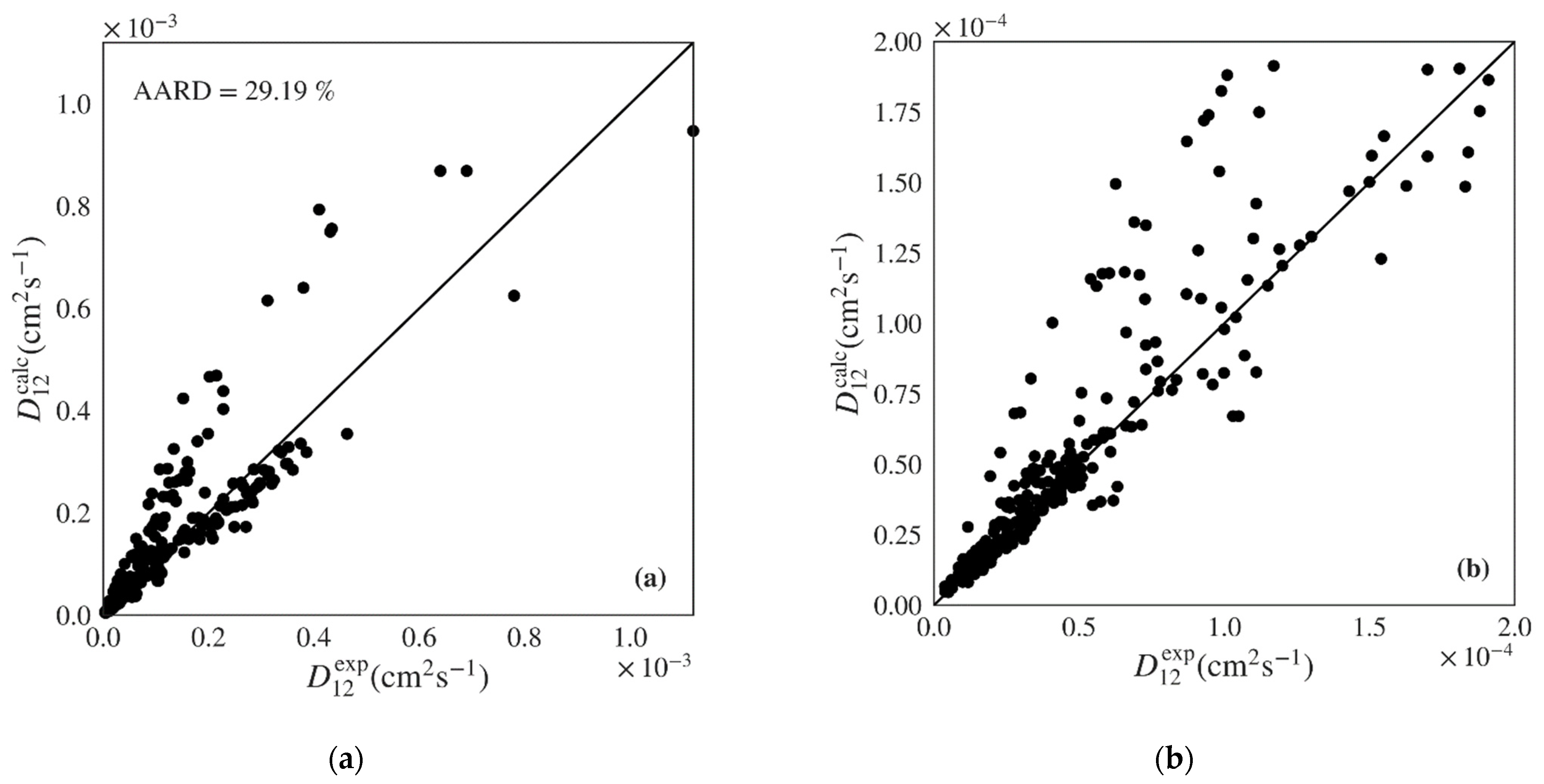
| Wilke-Chang | 130 | 342 | 29.19 | 28.20 | 0.26 | 172.30 | 6.66 × 10⁻⁵ | 0.7214 (0.5546) |
| Tyn-Calus | 130 | 342 | 28.84 | 27.82 | 0.18 | 64.97 | 7.01 × 10⁻⁵ | 0.6909 (0.7465) |
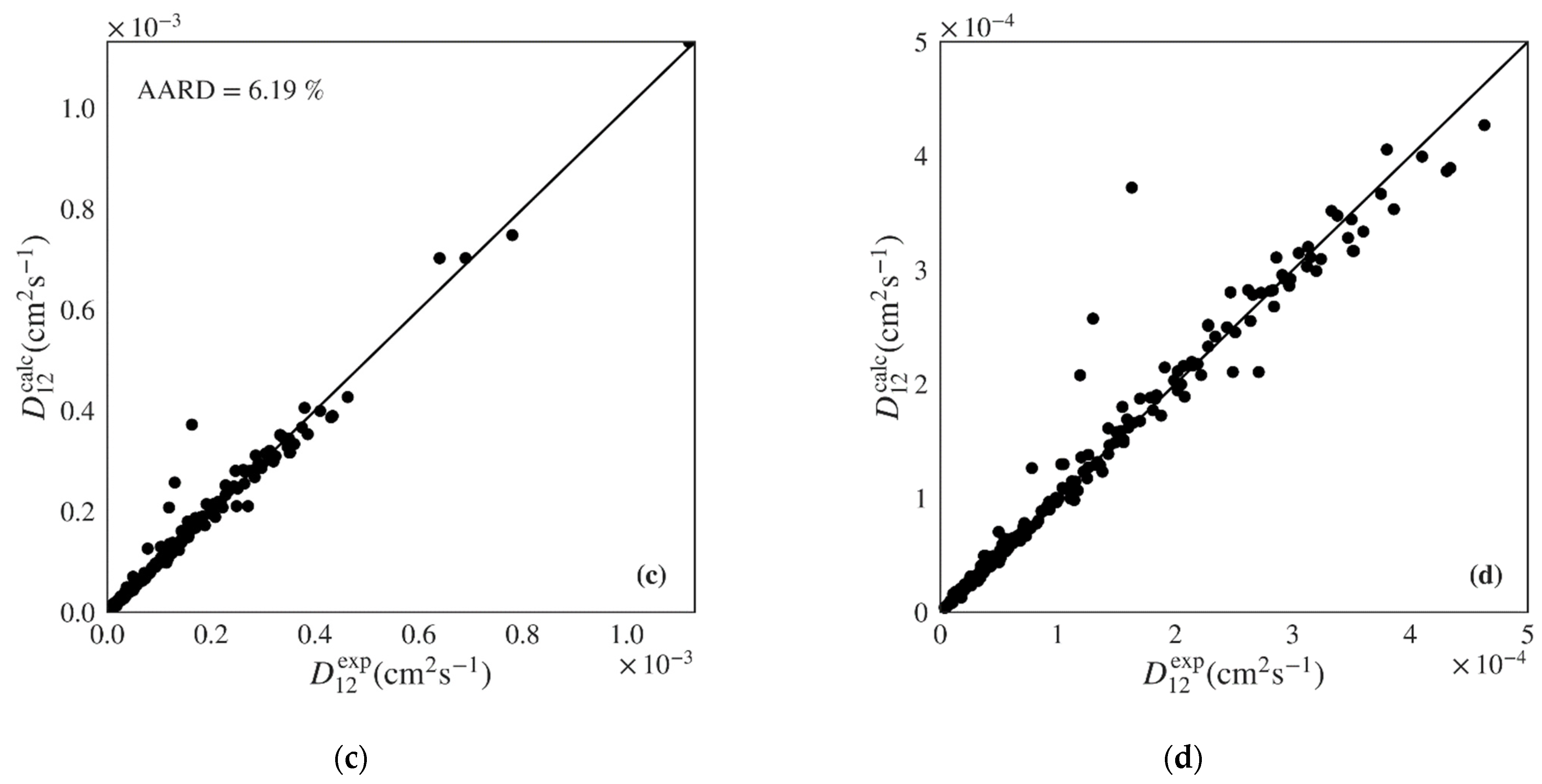
| Magalhães et al. | 125 * | 324 | 6.19 | 6.21 | 0.04 | 128.38 | 1.82 × 10⁻⁵ | 0.9801 (0.9890) |
| Zhu et al. | 130 | 342 | 37.93 | 45.19 | 1.40 | 222.45 | 6.35 × 10⁻⁵ | 0.7466 (0.8343) |
| NDP | AARD (%) | Data Ref. | |||||||||||
|---|---|---|---|---|---|---|---|---|---|---|---|---|---|
| ML Gradient Boosted | Wilke-Chang | Tyn-Calus | Magalhães et al. | ||||||||||
| Solvent | Solute | Total | Test | Train | Test | Train | Test | Train | Test | Train | Test | Train | |
| 1-propanol | ammonia | 31 | 14 | 17 | 5.65 | 0.60 | 33.93 | 31.25 | 19.49 | 21.11 | 4.53 | 2.23 | [71] |
| 1-propanol | carbon dioxide | 27 | 11 | 16 | 1.74 | 0.69 | 54.34 | 57.12 | 71.29 | 73.03 | 3.57 | 2.73 | [71] |
| 1-propanol | propane | 36 | 9 | 27 | 4.04 | 0.87 | 48.26 | 53.11 | 62.76 | 66.25 | 4.84 | 4.87 | [71] |
| 1-propanol | propene | 36 | 12 | 24 | 2.66 | 1.22 | 51.82 | 56.37 | 66.01 | 69.22 | 3.84 | 4.81 | [71] |
| 1-propanol | water | 5 | 2 | 3 | 38.77 | 0.16 | 153.58 | 119.30 | 46.19 | 26.42 | 18.77 | 0.93 | [72] |
| 2-propanol | benzene | 10 | 2 | 8 | 1.61 | 0.18 | 19.82 | 8.26 | 35.37 | 26.16 | 28.53 | 6.52 | [73] |
| 2-propanol | naphthalene | 10 | 3 | 7 | 0.93 | 0.23 | 7.64 | 13.02 | 24.72 | 24.05 | 9.06 | 10.74 | [73] |
| 2-propanol | n-decane | 10 | 3 | 7 | 0.74 | 0.20 | 11.68 | 20.45 | 23.09 | 30.72 | 3.81 | 15.80 | [73] |
| 2-propanol | n-tetradecane | 9 | 5 | 4 | 6.36 | 0.72 | 15.44 | 14.88 | 20.85 | 21.60 | 24.45 | 2.49 | [73] |
| 2-propanol | phenanthrene | 9 | 3 | 6 | 10.06 | 0.46 | 23.85 | 5.46 | 34.66 | 13.53 | 92.77 | 1.72 | [73] |
| 2-propanol | toluene | 10 | 1 | 9 | 7.16 | 0.19 | 18.91 | 9.87 | 36.94 | 26.77 | 13.69 | 8.03 | [73] |
| 2-propanol | water | 5 | 1 | 4 | 41.12 | 0.44 | 130.88 | 143.02 | 33.10 | 40.10 | 4.57 | 0.83 | [72] |
| acetone | 1,2,4-trichlorobenzene | 6 | 2 | 4 | 5.85 | 0.48 | 10.53 | 11.95 | 27.10 | 28.26 | 3.59 | 1.08 | [74] |
| acetone | 1,3,5-trimethylbenzene | 5 | 2 | 3 | 0.75 | 0.06 | 18.81 | 19.10 | 32.77 | 33.01 | 0.15 | 0.61 | [74] |
| acetone | benzene | 6 | 6 | 0.19 | 13.32 | 34.40 | 0.36 | [74] | |||||
| acetone | biphenyl | 6 | 1 | 5 | 4.35 | 0.63 | 18.79 | 18.79 | 30.99 | 30.99 | 0.46 | 0.40 | [74] |
| acetone | chlorobenzene | 6 | 6 | 0.14 | 13.57 | 32.58 | 0.85 | [74] | |||||
| acetone | ethylbenzene | 6 | 1 | 5 | 0.08 | 0.23 | 18.76 | 19.07 | 34.44 | 34.68 | 0.17 | 0.43 | [74] |
| acetone | naphthalene | 5 | 5 | 0.28 | 18.33 | 32.93 | 0.42 | [74] | |||||
| acetone | n-propylbenzene | 5 | 4 | 1 | 0.98 | 0.00 | 21.09 | 21.14 | 34.47 | 34.52 | [74] | ||
| acetone | toluene | 5 | 5 | 0.12 | 16.89 | 34.87 | 0.38 | [74] | |||||
| acetone | water | 4 | 1 | 3 | 5.94 | 0.06 | 83.53 | 85.64 | 6.60 | 7.82 | 0.80 | 0.87 | [75] |
| acetonitrile | [Bmim][bti] | 5 | 1 | 4 | 2.19 | 0.51 | 50.27 | 49.10 | 48.63 | 47.43 | 0.60 | 1.19 | [76] |
| acetonitrile | [Emim][bti] | 5 | 1 | 4 | 1.63 | 0.02 | 47.83 | 46.64 | 47.25 | 46.06 | 1.10 | 1.35 | [76] |
| acetonitrile | [Hmim][bti] | 5 | 5 | 0.29 | 48.77 | 46.06 | 1.94 | [76] | |||||
| acetonitrile | [Omim][bti] | 5 | 1 | 4 | 1.12 | 0.26 | 48.99 | 49.22 | 45.36 | 45.61 | 0.18 | 1.04 | [76] |
| acetonitrile | carbon disulfide | 5 | 3 | 2 | 16.39 | 3.76 | 22.64 | 28.64 | 41.91 | 46.42 | 10.72 | [77] | |
| acetonitrile | methanol | 20 | 6 | 14 | 6.49 | 0.96 | 20.28 | 15.79 | 43.25 | 40.05 | 1.44 | 1.78 | [77] |
| chlorobenzene | propene | 32 | 9 | 23 | 0.95 | 0.25 | 9.43 | 9.88 | 32.77 | 32.49 | 1.01 | 1.12 | [78,79] |
| chlorotrifluoromethane | 1,3-dibromobenzene | 12 | 3 | 9 | 9.31 | 1.21 | 147.23 | 148.48 | 75.18 | 76.06 | 6.85 | 4.14 | [80] |
| chlorotrifluoromethane | acetone | 10 | 2 | 8 | 16.17 | 0.78 | 93.87 | 93.66 | 24.18 | 24.05 | 8.00 | 3.55 | [80] |
| chlorotrifluoromethane | p-xylene | 8 | 1 | 7 | 7.05 | 0.65 | 75.61 | 98.40 | 24.84 | 41.04 | 2.31 | 3.68 | [80] |
| deuterium oxide | oxygen | 18 | 7 | 11 | 5.43 | 0.27 | 20.33 | 16.57 | 38.87 | 35.99 | 4.64 | 7.55 | [81] |
| ethanol | 1,2-butanediol | 5 | 2 | 3 | 37.20 | 1.27 | 30.65 | 27.41 | 13.27 | 15.42 | 2.61 | 0.24 | [82] |
| ethanol | 1,3,5-trimethylbenzene | 13 | 5 | 8 | 4.09 | 0.54 | 13.22 | 18.95 | 21.13 | 19.42 | 1.65 | 1.92 | [83] |
| ethanol | 1,4-butanediol | 4 | 4 | 63.79 | 48.40 | 2.88 | [82] | ||||||
| ethanol | 1-butanol | 4 | 3 | 1 | 20.44 | 3.64 | 17.25 | 17.95 | 22.96 | 22.49 | [82] | ||
| ethanol | 2-phenylethyl acetate | 15 | 4 | 11 | 2.64 | 1.38 | 16.89 | 17.80 | 38.86 | 39.53 | 2.98 | 1.97 | [84] |
| ethanol | 3-phenylpropyl acetate | 15 | 3 | 12 | 2.59 | 0.91 | 14.30 | 13.49 | 35.82 | 35.21 | 3.93 | 1.76 | [84] |
| ethanol | ammonia | 18 | 5 | 13 | 3.84 | 2.00 | 36.24 | 42.92 | 29.11 | 25.63 | 5.32 | 3.18 | [71] |
| ethanol | benzene | 21 | 8 | 13 | 3.42 | 1.16 | 27.35 | 24.37 | 25.74 | 35.54 | 6.16 | 12.16 | [82,83] |
| ethanol | benzonitrile | 16 | 8 | 8 | 1.86 | 0.97 | 24.97 | 25.34 | 48.86 | 49.11 | 0.83 | 1.02 | [85] |
| ethanol | benzyl acetate | 15 | 5 | 10 | 4.43 | 0.98 | 17.97 | 13.93 | 41.27 | 38.38 | 3.36 | 2.89 | [84] |
| ethanol | carbon dioxide | 27 | 9 | 18 | 4.82 | 2.21 | 49.74 | 46.56 | 72.64 | 70.90 | 5.08 | 3.73 | [71] |
| ethanol | chromium(III) acetylacetonate | 9 | 1 | 8 | 7.17 | 0.77 | 20.79 | 16.81 | 8.31 | 11.33 | 2.99 | 2.24 | [86,87] |
| ethanol | dibenzyl ether | 15 | 5 | 10 | 3.00 | 1.52 | 22.47 | 25.90 | 41.47 | 44.06 | 4.26 | 1.37 | [84] |
| ethanol | disperse blue 14 | 8 | 2 | 6 | 2.75 | 5.23 | 22.10 | 22.73 | 38.77 | 39.26 | 5.61 | 10.24 | [88] |
| ethanol | disperse orange 11 | 12 | 2 | 10 | 0.44 | 0.17 | 20.42 | 15.17 | 38.89 | 34.86 | 6.15 | 2.75 | [88] |
| ethanol | ethylene glycol | 5 | 2 | 3 | 76.23 | 0.05 | 61.03 | 57.90 | 4.28 | 2.65 | 5.06 | 1.36 | [82] |
| ethanol | eucalyptol | 12 | 4 | 8 | 7.02 | 1.06 | 10.58 | 13.85 | 34.55 | 36.94 | 0.48 | 0.65 | [56] |
| ethanol | gallic acid | 24 | 5 | 19 | 5.14 | 0.61 | 134.06 | 132.71 | 53.92 | 53.04 | 1.57 | 0.79 | [57] |
| ethanol | glycerol | 5 | 5 | 1.08 | 52.51 | 4.59 | 3.28 | [82] | |||||
| ethanol | Ibuprofen | 16 | 7 | 9 | 4.87 | 1.07 | 4.97 | 5.51 | 19.05 | 18.63 | 0.92 | 0.81 | [89] |
| ethanol | naphthalene | 13 | 2 | 11 | 8.86 | 0.16 | 21.43 | 14.25 | 30.88 | 20.36 | 11.33 | 1.13 | [83] |
| ethanol | nitrous oxide | 5 | 5 | 0.26 | 44.94 | 69.83 | 0.68 | [90] | |||||
| ethanol | palladium(II) acetylacetonate | 4 | 1 | 3 | 4.84 | 0.03 | 15.52 | 18.85 | 17.74 | 15.36 | 0.67 | 0.80 | [87] |
| ethanol | phenanthrene | 13 | 2 | 11 | 11.23 | 0.06 | 4.25 | 11.34 | 22.56 | 17.30 | 2.83 | 1.26 | [83] |
| ethanol | phenylbutazone | 8 | 1 | 7 | 7.87 | 2.02 | 10.27 | 10.72 | 10.26 | 9.89 | 2.01 | 2.13 | [91] |
| ethanol | propane | 30 | 7 | 23 | 4.31 | 1.93 | 43.06 | 42.56 | 64.52 | 64.21 | 7.48 | 8.90 | [71] |
| ethanol | propene | 30 | 5 | 25 | 1.78 | 1.52 | 43.30 | 45.74 | 65.37 | 66.86 | 7.80 | 7.72 | [71] |
| ethanol | quercetin | 16 | 6 | 10 | 7.15 | 1.79 | 40.58 | 40.59 | 9.60 | 9.61 | 0.86 | 1.11 | [92] |
| ethanol | toluene | 14 | 7 | 7 | 5.02 | 0.12 | 20.45 | 17.54 | 24.14 | 20.86 | 8.93 | 0.70 | [83] |
| ethanol | water | 15 | 2 | 13 | 15.26 | 0.90 | 131.04 | 145.20 | 15.31 | 22.37 | 4.86 | 4.30 | [75,82,93] |
| ethyl acetate | astaxanthin | 12 | 5 | 7 | 1.50 | 0.56 | 11.44 | 14.29 | 8.83 | 11.61 | 1.51 | 2.85 | [94] |
| ethyl acetate | quercetin | 16 | 4 | 12 | 2.90 | 0.52 | 44.69 | 50.17 | 19.78 | 24.31 | 3.18 | 1.80 | [92] |
| ethyl acetate | squalene | 12 | 2 | 10 | 2.01 | 0.57 | 7.70 | 8.86 | 12.34 | 13.44 | 1.54 | 0.98 | [94] |
| ethylene glycol | propene | 31 | 9 | 22 | 1.36 | 0.86 | 48.94 | 48.81 | 64.24 | 64.14 | 1.41 | 1.70 | [78,79] |
| methanol | [Bmim][bti] | 11 | 5 | 6 | 3.46 | 1.69 | 42.58 | 41.65 | 54.56 | 53.82 | 5.00 | 2.15 | [76,95] |
| methanol | [Emim][bti] | 11 | 4 | 7 | 5.07 | 0.23 | 40.25 | 41.85 | 53.72 | 54.96 | 5.24 | 1.64 | [76,95] |
| methanol | [Hmim][bti] | 5 | 2 | 3 | 4.25 | 0.54 | 36.57 | 39.04 | 48.83 | 50.82 | 3.91 | 0.74 | [76] |
| methanol | [Omim][bti] | 5 | 5 | 0.61 | 39.02 | 49.96 | 1.33 | [76] | |||||
| methanol | 1,3,5-trimethylbenzene | 4 | 4 | 1.15 | 15.85 | 42.38 | 3.25 | [73] | |||||
| methanol | acetonitrile | 26 | 9 | 17 | 2.94 | 1.30 | 27.88 | 26.50 | 57.94 | 57.13 | 2.19 | 1.63 | [77] |
| methanol | ammonia | 24 | 6 | 18 | 0.93 | 1.78 | 106.11 | 114.44 | 3.67 | 7.78 | 4.25 | 3.93 | [71] |
| methanol | benzene | 4 | 1 | 3 | 2.79 | 0.55 | 1.88 | 12.49 | 38.59 | 45.23 | 3.28 | 4.28 | [73] |
| methanol | carbon dioxide | 25 | 10 | 15 | 3.80 | 0.79 | 30.72 | 30.86 | 63.70 | 63.77 | 4.05 | 3.84 | [71] |
| methanol | carbon monoxide | 8 | 1 | 7 | 4.88 | 0.52 | 23.36 | 14.78 | 59.89 | 55.02 | 8.75 | 3.60 | [96] |
| methanol | disperse blue 14 | 8 | 2 | 6 | 3.70 | 0.59 | 57.69 | 51.97 | 67.99 | 63.66 | 8.22 | 1.11 | [88] |
| methanol | disperse orange 11 | 16 | 5 | 11 | 2.65 | 0.26 | 51.25 | 52.71 | 63.97 | 65.05 | 3.01 | 1.96 | [88] |
| methanol | naphthalene | 4 | 2 | 2 | 7.59 | 0.08 | 17.60 | 15.98 | 44.04 | 42.94 | 19.90 | [73] | |
| methanol | p-chloronitrobenzene | 18 | 7 | 11 | 1.47 | 0.60 | 22.46 | 22.66 | 46.93 | 47.06 | 1.08 | 1.07 | [97] |
| methanol | phenanthrene | 4 | 1 | 3 | 13.71 | 0.48 | 12.15 | 21.29 | 37.19 | 43.73 | 4.44 | 3.14 | [73] |
| methanol | propane | 27 | 11 | 16 | 2.14 | 1.50 | 24.08 | 27.00 | 54.47 | 56.22 | 2.43 | 2.45 | [71] |
| methanol | toluene | 4 | 4 | 0.25 | 14.12 | 44.35 | 3.66 | [73] | |||||
| methanol | vitamin K3 | 4 | 4 | 0.45 | 25.59 | 47.09 | 0.45 | [98] | |||||
| methanol | water | 5 | 2 | 3 | 28.86 | 0.74 | 310.36 | 281.35 | 97.11 | 83.18 | 11.09 | 0.18 | [99] |
| n-butanol | ammonia | 64 | 17 | 47 | 2.63 | 1.75 | 38.12 | 38.41 | 20.73 | 20.56 | 5.36 | 5.81 | [71] |
| n-butanol | carbon dioxide | 66 | 19 | 47 | 1.19 | 1.06 | 47.26 | 45.51 | 68.33 | 67.28 | 5.98 | 6.27 | [71] |
| n-butanol | propane | 98 | 33 | 65 | 1.86 | 1.51 | 49.70 | 49.52 | 65.43 | 65.31 | 2.58 | 3.15 | [71] |
| n-butanol | propene | 135 | 45 | 90 | 2.83 | 1.66 | 50.48 | 48.53 | 66.64 | 65.33 | 5.15 | 3.90 | [71] |
| Solvent | Solute | NDP | AARD (%) | Data Ref. | |||||||||||
|---|---|---|---|---|---|---|---|---|---|---|---|---|---|---|---|
| ML Gradient Boosted | Wilke-Chang | Tyn-Calus | Magalhães et al. | Zhu et al. | |||||||||||
| Total | Test | Train | Test | Train | Test | Train | Test | Train | Test | Train | Test | Train | |||
| 2,2,4-trimethylpentane | 1,3,5-trimethylbenzene | 4 | 4 | 2.11 | 21.44 | 17.70 | 0.64 | 171.90 | [100] | ||||||
| 2,2,4-trimethylpentane | benzene | 4 | 1 | 3 | 2.49 | 1.36 | 11.31 | 14.98 | 31.05 | 28.78 | 0.04 | 2.33 | 128.60 | 119.69 | [100] |
| 2,2,4-trimethylpentane | ethylbenzene | 4 | 4 | 3.68 | 19.42 | 21.11 | 1.79 | 157.43 | [100] | ||||||
| 2,2,4-trimethylpentane | o-xylene | 4 | 4 | 1.96 | 16.19 | 23.43 | 2.78 | 147.48 | [100] | ||||||
| 2,2,4-trimethylpentane | p-xylene | 4 | 1 | 3 | 6.04 | 6.76 | 15.57 | 5.11 | 23.48 | 33.84 | 4.27 | 2.74 | 116.04 | 126.93 | [100] |
| 2,2,4-trimethylpentane | toluene | 4 | 4 | 2.21 | 10.10 | 29.38 | 2.07 | 126.50 | [100] | ||||||
| 2,3-dimethylbutane | benzene | 11 | 2 | 9 | 3.22 | 3.10 | 14.74 | 13.29 | 40.85 | 39.84 | 1.78 | 1.74 | 9.45 | 7.59 | [101] |
| 2,3-dimethylbutane | naphthalene | 9 | 2 | 7 | 1.28 | 1.68 | 18.35 | 19.02 | 38.53 | 39.04 | 0.61 | 2.18 | 1.80 | 2.59 | [101] |
| 2,3-dimethylbutane | phenanthrene | 11 | 2 | 9 | 0.65 | 0.63 | 20.75 | 20.51 | 37.19 | 36.99 | 2.44 | 1.63 | 2.39 | 5.87 | [101] |
| 2,3-dimethylbutane | toluene | 10 | 2 | 8 | 2.52 | 3.36 | 15.89 | 17.53 | 39.58 | 40.75 | 2.84 | 2.17 | 4.97 | 4.77 | [101] |
| cyclohexane | 1,1′-dimethylferrocene | 5 | 2 | 3 | 1.07 | 1.64 | 9.73 | 8.30 | 17.40 | 18.48 | 2.41 | 0.26 | 192.52 | 197.96 | [102] |
| cyclohexane | 1,3,5-trimethylbenzene | 12 | 1 | 11 | 9.04 | 3.82 | 6.73 | 14.13 | 28.83 | 14.33 | 8.28 | 8.32 | 16.07 | 59.79 | [103,104] |
| cyclohexane | acetone | 4 | 2 | 2 | 2.31 | 0.01 | 20.96 | 19.77 | 46.91 | 46.10 | 0.96 | 106.99 | 92.31 | [104] | |
| cyclohexane | argon | 7 | 3 | 4 | 9.78 | 4.63 | 6.89 | 2.54 | 43.32 | 44.85 | 5.54 | 2.05 | 40.33 | 66.48 | [105] |
| cyclohexane | benzene | 12 | 2 | 10 | 12.00 | 2.96 | 24.55 | 17.57 | 13.13 | 18.78 | 12.40 | 8.05 | 92.05 | 61.13 | [104,106] |
| cyclohexane | carbon tetrachloride | 7 | 2 | 5 | 0.50 | 1.02 | 15.04 | 23.35 | 18.88 | 13.02 | 3.28 | 0.96 | 53.23 | 103.63 | [105] |
| cyclohexane | ethane | 5 | 1 | 4 | 13.53 | 1.23 | 3.43 | 2.22 | 34.57 | 37.18 | 0.29 | 1.23 | 183.33 | 86.88 | [107] |
| cyclohexane | ethylene | 5 | 1 | 4 | 1.93 | 1.06 | 0.26 | 1.74 | 37.99 | 37.80 | 1.60 | 1.08 | 66.73 | 110.83 | [107] |
| cyclohexane | ethylferrocene | 6 | 1 | 5 | 0.68 | 0.49 | 5.53 | 8.18 | 20.56 | 18.56 | 1.18 | 0.75 | 178.04 | 169.05 | [102] |
| cyclohexane | ferrocene | 5 | 3 | 2 | 2.84 | 0.08 | 15.24 | 13.62 | 16.70 | 17.87 | 1.37 | 0.20 | 49.79 | 58.60 | [102] |
| cyclohexane | krypton | 6 | 3 | 3 | 9.01 | 2.60 | 16.32 | 15.16 | 32.42 | 33.09 | 3.07 | 1.27 | 54.85 | 78.43 | [105] |
| cyclohexane | methane | 6 | 4 | 2 | 13.80 | 0.41 | 9.74 | 9.08 | 46.78 | 46.39 | 7.63 | 49.30 | 22.59 | [105] | |
| cyclohexane | m-xylene | 4 | 4 | 1.01 | 21.96 | 41.90 | 1.29 | 94.56 | [104] | ||||||
| cyclohexane | naphthalene | 12 | 4 | 8 | 10.33 | 3.64 | 14.64 | 10.87 | 14.91 | 18.18 | 9.98 | 6.90 | 41.94 | 39.98 | [104,106] |
| cyclohexane | phenanthrene | 8 | 3 | 5 | 5.64 | 1.43 | 4.82 | 4.27 | 19.02 | 23.03 | 4.82 | 2.49 | 4.34 | 7.53 | [106] |
| cyclohexane | p-xylene | 8 | 8 | 2.31 | 4.13 | 28.00 | 3.63 | 28.67 | [106] | ||||||
| cyclohexane | tetrabutyltin | 7 | 2 | 5 | 10.03 | 1.38 | 20.87 | 25.56 | 7.51 | 9.58 | 3.79 | 1.64 | 11.64 | 14.39 | [105] |
| cyclohexane | tetraethyltin | 7 | 2 | 5 | 0.61 | 1.78 | 24.37 | 24.29 | 7.91 | 8.24 | 1.43 | 2.17 | 57.43 | 57.01 | [105] |
| cyclohexane | tetramethyltin | 7 | 2 | 5 | 4.77 | 0.48 | 29.90 | 33.82 | 9.13 | 7.47 | 2.31 | 1.06 | 90.37 | 95.59 | [105] |
| cyclohexane | tetrapropyltin | 6 | 4 | 2 | 3.96 | 1.01 | 21.89 | 30.99 | 7.23 | 8.08 | 2.03 | 21.99 | 21.49 | [105] | |
| cyclohexane | toluene | 12 | 2 | 10 | 8.49 | 3.06 | 16.22 | 10.84 | 18.75 | 20.21 | 11.65 | 7.31 | 51.76 | 56.57 | [104,106] |
| cyclohexane | xenon | 7 | 6 | 1 | 5.42 | 0.02 | 25.17 | 14.32 | 23.88 | 30.48 | 83.09 | 150.96 | [105] | ||
| ethane | 1-octene | 6 | 2 | 4 | 6.96 | 1.27 | 3.27 | 5.54 | 1.86 | 5.43 | 5.88 | 1.96 | 17.16 | 9.15 | [108] |
| ethane | 1-tetradecene | 9 | 4 | 5 | 6.06 | 0.28 | 20.10 | 20.84 | 13.67 | 14.48 | 3.84 | 3.71 | 21.78 | 13.41 | [108] |
| n-decane | 12-crown-4 | 4 | 1 | 3 | 8.73 | 4.44 | 20.77 | 23.64 | 17.52 | 15.56 | 0.66 | 4.99 | 42.67 | 40.09 | [109] |
| n-decane | 15-crown-5 | 4 | 1 | 3 | 8.77 | 1.24 | 41.39 | 22.03 | 0.18 | 13.54 | 22.17 | 0.69 | 28.31 | 21.11 | [109] |
| n-decane | 18-crown-6 | 4 | 1 | 3 | 2.17 | 2.05 | 30.58 | 25.53 | 4.63 | 8.31 | 14.50 | 4.29 | 3.54 | 4.36 | [109] |
| n-decane | argon | 3 | 2 | 1 | 11.89 | 0.11 | 12.79 | 10.56 | 44.32 | 55.28 | 26.35 | 91.32 | [110] | ||
| n-decane | carbon tetrachloride | 3 | 3 | 5.74 | 17.09 | 26.45 | 1.24 | 71.87 | [110] | ||||||
| n-decane | dicyclohexano-18-crown-6 | 4 | 4 | 0.68 | 25.60 | 2.44 | 1.27 | 83.59 | [109] | ||||||
| n-decane | dicyclohexano-24-crown-8 | 4 | 3 | 1 | 7.95 | 0.13 | 25.82 | 33.28 | 3.15 | 8.46 | 119.04 | 192.36 | [109] | ||
| n-decane | krypton | 3 | 3 | 2.49 | 23.85 | 35.90 | 3.27 | 69.93 | [110] | ||||||
| n-decane | s-trioxane | 4 | 4 | 2.24 | 24.60 | 25.63 | 0.91 | 50.71 | [109] | ||||||
| n-decane | tetrabutyltin | 4 | 1 | 3 | 3.53 | 0.71 | 29.41 | 29.09 | 2.91 | 3.22 | 1.57 | 0.96 | 22.54 | 20.34 | [110] |
| n-decane | tetraethyltin | 4 | 1 | 3 | 25.87 | 24.86 | 1.63 | 6.66 | 33.23 | 30.98 | 0.59 | 1.98 | 19.15 | 13.44 | [110] |
| n-decane | tetramethyltin | 4 | 2 | 2 | 4.38 | 7.90 | 37.59 | 36.56 | 14.25 | 14.90 | 2.61 | 75.10 | 68.10 | [110] | |
| n-decane | tetrapropyltin | 4 | 1 | 3 | 0.83 | 1.65 | 26.81 | 29.97 | 8.87 | 6.60 | 0.68 | 2.00 | 26.72 | 24.34 | [110] |
| n-decane | xenon | 8 | 1 | 7 | 15.12 | 2.57 | 1.46 | 18.76 | 46.61 | 35.66 | 5.99 | 3.19 | 137.71 | 82.50 | [110,111] |
| n-dodecane | 1,3,5-trimethylbenzene | 4 | 2 | 2 | 4.64 | 0.31 | 6.99 | 1.70 | 39.23 | 35.47 | 3.02 | 130.38 | 107.10 | [104] | |
| n-dodecane | acetone | 5 | 1 | 4 | 6.18 | 0.82 | 5.13 | 4.64 | 45.44 | 45.15 | 0.90 | 1.37 | 98.06 | 103.24 | [104] |
| n-dodecane | benzene | 4 | 2 | 2 | 3.42 | 0.69 | 4.97 | 3.88 | 43.25 | 42.60 | 1.57 | 0.00 | 122.78 | 121.55 | [104] |
| n-dodecane | carbon dioxide | 9 | 3 | 6 | 5.85 | 2.86 | 61.83 | 88.25 | 19.08 | 9.16 | 11.39 | 1.56 | 30.14 | 22.67 | [112] |
| n-dodecane | carbon monoxide | 9 | 3 | 6 | 15.15 | 2.87 | 73.13 | 52.06 | 13.55 | 24.07 | 7.28 | 7.69 | 24.57 | 29.78 | [112] |
| n-dodecane | hydrogen | 9 | 5 | 4 | 7.78 | 6.84 | 25.13 | 21.17 | 64.97 | 63.11 | 10.12 | 9.67 | 47.72 | 49.66 | [112] |
| n-dodecane | linoleic acid methyl ester | 4 | 4 | 1.10 | 13.54 | 13.08 | 0.37 | 42.50 | [104] | ||||||
| n-dodecane | m-xylene | 4 | 4 | 1.39 | 10.17 | 42.74 | 0.62 | 108.09 | [104] | ||||||
| n-dodecane | naphthalene | 5 | 2 | 3 | 4.99 | 0.75 | 5.64 | 10.11 | 38.86 | 41.75 | 3.55 | 0.93 | 79.40 | 81.82 | [104] |
| n-dodecane | n-decane | 5 | 1 | 4 | 0.03 | 2.21 | 56.61 | 45.00 | 8.43 | 4.59 | 1.98 | 3.71 | 11.30 | 34.63 | [113] |
| n-dodecane | n-hexadecane | 5 | 1 | 4 | 10.77 | 1.08 | 65.59 | 57.28 | 23.68 | 17.47 | 5.92 | 0.83 | 19.21 | 19.32 | [113] |
| n-dodecane | n-octane | 9 | 6 | 3 | 2.31 | 0.16 | 47.87 | 50.94 | 6.18 | 3.73 | 10.34 | 1.17 | 33.86 | 8.63 | [113] |
| n-dodecane | n-tetradecane | 5 | 1 | 4 | 2.94 | 1.23 | 39.89 | 59.70 | 2.42 | 16.92 | 16.34 | 1.53 | 20.35 | 16.40 | [113] |
| n-dodecane | toluene | 4 | 2 | 2 | 5.84 | 0.79 | 7.90 | 11.57 | 43.05 | 45.33 | 2.72 | 95.30 | 125.51 | [104] | |
| n-dodecane | vitamin K3 | 4 | 1 | 3 | 0.19 | 0.22 | 10.31 | 11.59 | 39.14 | 40.01 | 0.22 | 0.98 | 34.63 | 38.39 | [104] |
| n-eicosane | carbon dioxide | 5 | 2 | 3 | 16.17 | 0.01 | 172.30 | 147.95 | 21.79 | 12.93 | 0.71 | 1.13 | 8.06 | 29.92 | [114] |
| n-eicosane | carbon monoxide | 5 | 2 | 3 | 10.88 | 4.29 | 114.69 | 136.89 | 8.76 | 7.81 | 0.55 | 0.54 | 50.15 | 19.59 | [114] |
| n-eicosane | hydrogen | 5 | 1 | 4 | 3.25 | 110.78 | 8.54 | 252.32 | 61.72 | 129.43 | 128.38 | 73.30 | 4.12 | 99.16 | [114] |
| n-eicosane | n-dodecane | 5 | 2 | 3 | 13.72 | 1.97 | 138.63 | 134.49 | 52.19 | 49.55 | 1.74 | 0.91 | 67.82 | 55.95 | [114] |
| n-eicosane | n-hexadecane | 5 | 4 | 1 | 16.16 | 1.99 | 141.26 | 144.68 | 61.19 | 63.48 | 61.96 | 30.75 | [114] | ||
| n-eicosane | n-octane | 5 | 2 | 3 | 7.53 | 0.63 | 134.16 | 124.83 | 39.95 | 34.37 | 2.54 | 1.67 | 54.76 | 57.07 | [114] |
| n-heptane | 1,3,5-trimethylbenzene | 4 | 2 | 2 | 0.87 | 0.75 | 4.11 | 5.33 | 23.55 | 22.65 | 1.43 | 7.92 | 9.31 | [115] | |
| n-heptane | 2,2,4-trimethylpentane | 4 | 2 | 2 | 4.54 | 0.52 | 1.39 | 2.85 | 24.53 | 23.44 | 0.58 | 0.10 | 23.40 | 21.87 | [116] |
| n-heptane | benzene | 11 | 4 | 7 | 3.62 | 2.15 | 4.50 | 6.14 | 29.86 | 28.76 | 1.91 | 3.07 | 8.71 | 12.97 | [115,117] |
| n-heptane | ethylbenzene | 4 | 4 | 5.10 | 8.27 | 22.51 | 0.23 | 14.85 | [115] | ||||||
| n-heptane | n-decane | 6 | 1 | 5 | 4.29 | 2.79 | 15.13 | 6.99 | 33.96 | 24.47 | 8.69 | 2.42 | 10.94 | 5.52 | [113,118] |
| n-heptane | n-dodecane | 6 | 3 | 3 | 5.28 | 0.14 | 4.41 | 14.00 | 19.20 | 31.09 | 59.49 | 2.21 | 6.13 | 24.60 | [113,118] |
| n-heptane | n-hexadecane | 9 | 3 | 6 | 6.51 | 0.65 | 5.88 | 5.39 | 17.14 | 16.55 | 1.00 | 1.38 | 26.09 | 25.64 | [119,120,121] |
| n-heptane | n-hexane | 11 | 3 | 8 | 5.03 | 0.79 | 8.45 | 10.02 | 34.59 | 35.72 | 2.67 | 0.77 | 16.44 | 10.75 | [113,119,121] |
| n-heptane | n-octane | 13 | 3 | 10 | 7.32 | 1.72 | 7.36 | 9.29 | 27.53 | 31.88 | 2.94 | 1.28 | 4.50 | 2.94 | [113,118] |
| n-heptane | n-tetradecane | 6 | 3 | 3 | 2.73 | 1.12 | 7.65 | 9.45 | 21.46 | 22.01 | 2.56 | 1.51 | 28.62 | 33.71 | [113,118] |
| n-heptane | o-xylene | 4 | 2 | 2 | 4.35 | 2.02 | 7.08 | 2.49 | 29.03 | 29.16 | 0.62 | 3.70 | 3.50 | [115] | |
| n-heptane | p-xylene | 4 | 1 | 3 | 6.86 | 2.70 | 5.35 | 7.22 | 32.10 | 33.44 | 0.70 | 0.66 | 1.40 | 1.36 | [115] |
| n-heptane | toluene | 4 | 3 | 1 | 5.71 | 1.04 | 3.63 | 5.00 | 33.00 | 27.03 | 4.30 | 5.86 | [115] | ||
| n-hexadecane | carbon dioxide | 10 | 4 | 6 | 2.02 | 1.81 | 92.63 | 112.99 | 13.75 | 15.19 | 7.11 | 4.53 | 37.48 | 32.03 | [112] |
| n-hexadecane | carbon monoxide | 10 | 3 | 7 | 3.49 | 3.59 | 80.63 | 91.32 | 16.76 | 13.82 | 3.77 | 4.83 | 52.93 | 49.96 | [112] |
| n-hexadecane | hydrogen | 10 | 7 | 3 | 6.89 | 1.04 | 24.77 | 18.43 | 59.19 | 54.00 | 12.88 | 0.99 | 38.66 | 34.17 | [112] |
| n-hexadecane | n-decane | 5 | 1 | 4 | 10.89 | 1.40 | 62.63 | 79.23 | 5.76 | 16.55 | 5.16 | 1.59 | 152.48 | 39.94 | [122] |
| n-hexadecane | n-dodecane | 5 | 5 | 1.16 | 75.79 | 17.71 | 2.72 | 55.76 | [122] | ||||||
| n-hexadecane | n-octane | 10 | 1 | 9 | 6.82 | 0.57 | 88.97 | 76.42 | 18.59 | 10.71 | 1.45 | 3.00 | 22.13 | 68.70 | [122] |
| n-hexadecane | n-tetradecane | 5 | 2 | 3 | 1.59 | 1.09 | 70.97 | 78.33 | 17.57 | 22.63 | 2.13 | 2.39 | 50.42 | 36.41 | [122] |
| n-hexane | 1,1′-dimethylferrocene | 4 | 1 | 3 | 0.96 | 0.27 | 15.92 | 16.74 | 13.20 | 12.58 | 1.01 | 0.08 | 45.28 | 46.51 | [102] |
| n-hexane | 1,2,3,5-tetrafluorobenzene | 7 | 2 | 5 | 4.31 | 3.24 | 20.21 | 17.52 | 41.62 | 39.64 | 1.22 | 5.13 | 7.14 | 10.04 | [123] |
| n-hexane | 1,2,4,5-tetrafluorobenzene | 7 | 2 | 5 | 1.98 | 1.25 | 20.44 | 16.25 | 41.78 | 38.72 | 3.09 | 4.44 | 13.93 | 16.22 | [123] |
| n-hexane | 1,2,4-trifluorobenzene | 7 | 2 | 5 | 4.61 | 0.87 | 24.28 | 14.88 | 45.04 | 38.22 | 5.76 | 1.46 | 12.96 | 6.40 | [123] |
| n-hexane | 1,3,5-trimethylbenzene | 20 | 7 | 13 | 2.98 | 1.59 | 10.09 | 8.34 | 31.66 | 30.42 | 5.24 | 5.79 | 8.52 | 4.45 | [103,104] |
| n-hexane | 9,10-dimethylanthracene | 8 | 4 | 4 | 13.89 | 3.00 | 12.79 | 19.02 | 27.56 | 32.73 | 6.22 | 0.32 | 116.02 | 83.34 | [124] |
| n-hexane | acetone | 5 | 2 | 3 | 2.70 | 1.08 | 5.05 | 3.73 | 36.55 | 34.67 | 5.60 | 1.05 | 10.75 | 4.24 | [104] |
| n-hexane | acetonitrile | 7 | 7 | 2.40 | 5.79 | 39.09 | 2.70 | 22.16 | [125] | ||||||
| n-hexane | benzene | 48 | 18 | 30 | 3.48 | 2.39 | 6.16 | 7.86 | 31.07 | 31.34 | 9.04 | 6.60 | 15.66 | 25.65 | [103,104,107,123,125,126,127,128] |
| n-hexane | carbon disulfide | 10 | 4 | 6 | 4.49 | 3.58 | 2.32 | 10.16 | 35.24 | 29.75 | 7.20 | 3.52 | 44.88 | 76.81 | [125] |
| n-hexane | carbon tetrabromide | 8 | 1 | 7 | 7.97 | 1.02 | 30.34 | 19.55 | 5.72 | 16.14 | 1.95 | 8.28 | 168.32 | 115.24 | [124] |
| n-hexane | ethylferrocene | 4 | 4 | 0.61 | 18.11 | 11.55 | 0.12 | 35.49 | [102] | ||||||
| n-hexane | ferrocene | 4 | 1 | 3 | 3.84 | 0.40 | 31.11 | 22.97 | 5.72 | 11.57 | 0.41 | 0.15 | 17.28 | 16.84 | [123] |
| n-hexane | hexafluorobenzene | 7 | 2 | 5 | 2.23 | 1.89 | 7.46 | 10.50 | 31.30 | 34.96 | 2.19 | 3.76 | 15.66 | 21.90 | [123] |
| n-hexane | indole | 2 | 2 | 0.62 | 10.64 | 32.22 | 13.24 | [104] | |||||||
| n-hexane | linoleic acid methyl ester | 2 | 2 | 2.02 | 2.08 | 12.90 | 95.99 | [104] | |||||||
| n-hexane | m-xylene | 5 | 2 | 3 | 1.77 | 0.04 | 9.32 | 8.01 | 32.84 | 31.87 | 1.82 | 2.56 | 5.26 | 4.57 | [104] |
| n-hexane | naphthalene | 21 | 5 | 16 | 3.43 | 2.44 | 12.23 | 11.95 | 33.92 | 33.71 | 4.95 | 4.32 | 8.19 | 10.88 | [103,104,125,126] |
| n-hexane | n-heptane | 11 | 5 | 6 | 4.88 | 1.16 | 13.00 | 12.35 | 29.03 | 33.49 | 7.30 | 0.93 | 13.25 | 2.53 | [119,120,121,129] |
| n-hexane | n-octane | 7 | 2 | 5 | 2.01 | 1.14 | 12.76 | 12.64 | 32.28 | 32.19 | 1.05 | 0.30 | 2.05 | 1.68 | [119,129] |
| n-hexane | octafluorotoluene | 7 | 1 | 6 | 0.23 | 0.26 | 21.39 | 8.53 | 40.45 | 30.16 | 4.30 | 2.92 | 13.40 | 15.97 | [123] |
| n-hexane | o-difluorobenzene | 7 | 2 | 5 | 2.25 | 0.86 | 9.72 | 12.64 | 35.75 | 37.83 | 4.29 | 2.44 | 3.57 | 16.35 | [123] |
| n-hexane | p-difluorobenzene | 7 | 3 | 4 | 2.62 | 0.44 | 19.67 | 9.73 | 42.83 | 35.76 | 24.35 | 0.79 | 27.69 | 2.93 | [123] |
| n-hexane | pentafluorobenzene | 7 | 1 | 6 | 2.79 | 0.39 | 1.84 | 12.11 | 26.52 | 36.58 | 1.96 | 3.78 | 6.06 | 17.91 | [123] |
| n-hexane | phenanthrene | 15 | 6 | 9 | 3.33 | 1.60 | 14.07 | 14.25 | 31.89 | 32.04 | 4.37 | 5.72 | 14.18 | 11.93 | [103] |
| n-hexane | p-xylene | 17 | 4 | 13 | 6.35 | 2.44 | 15.89 | 10.62 | 37.62 | 33.72 | 4.15 | 4.56 | 9.32 | 8.04 | [103,104] |
| n-hexane | pyrene | 8 | 2 | 6 | 10.54 | 10.51 | 62.03 | 50.27 | 31.35 | 21.81 | 8.62 | 4.72 | 153.51 | 103.03 | [124,126] |
| n-hexane | toluene | 32 | 14 | 18 | 4.58 | 2.65 | 8.46 | 8.14 | 32.19 | 30.74 | 4.98 | 3.72 | 12.56 | 19.33 | [103,104,130,131] |
| n-hexane | vitamin K3 | 5 | 1 | 4 | 3.32 | 1.01 | 11.31 | 16.36 | 30.09 | 34.07 | 0.78 | 0.73 | 34.19 | 37.24 | [104,132] |
| n-octane | 1,3,5-trimethylbenzene | 8 | 3 | 5 | 2.31 | 1.74 | 7.21 | 6.99 | 23.51 | 23.67 | 0.47 | 0.62 | 23.97 | 22.64 | [103,104] |
| n-octane | argon | 4 | 1 | 3 | 1.76 | 5.82 | 6.69 | 14.09 | 44.01 | 41.09 | 1.93 | 1.30 | 23.81 | 18.74 | [110] |
| n-octane | benzene | 8 | 2 | 6 | 1.90 | 0.79 | 2.80 | 2.87 | 34.64 | 35.64 | 0.29 | 0.20 | 15.45 | 17.40 | [100,115] |
| n-octane | carbon tetrachloride | 4 | 4 | 1.24 | 15.76 | 23.67 | 1.05 | 34.90 | [110] | ||||||
| n-octane | ethylbenzene | 8 | 4 | 4 | 6.65 | 6.50 | 3.65 | 7.21 | 28.14 | 25.44 | 3.22 | 1.19 | 24.94 | 22.80 | [100,115] |
| n-octane | krypton | 4 | 1 | 3 | 14.06 | 1.75 | 22.31 | 30.11 | 33.56 | 29.32 | 3.72 | 0.39 | 40.36 | 36.12 | [110] |
| n-octane | methane | 4 | 1 | 3 | 9.77 | 2.46 | 10.46 | 3.34 | 50.64 | 45.68 | 6.32 | 0.40 | 45.79 | 10.22 | [110] |
| n-octane | n-heptane | 7 | 4 | 3 | 6.34 | 0.55 | 11.43 | 11.60 | 36.84 | 36.96 | 1.42 | 0.12 | 20.87 | 17.70 | [119,133] |
| n-octane | n-hexane | 6 | 4 | 2 | 4.66 | 0.29 | 5.47 | 6.95 | 34.39 | 35.42 | 3.46 | 34.50 | 22.19 | [119] | |
| n-octane | o-xylene | 8 | 8 | 1.39 | 1.30 | 31.53 | 0.73 | 14.39 | [100,115] | ||||||
| n-octane | p-xylene | 8 | 1 | 7 | 5.49 | 3.85 | 9.50 | 8.80 | 36.92 | 36.43 | 0.99 | 0.83 | 4.21 | 7.47 | [100,115] |
| n-octane | tetrabutyltin | 4 | 1 | 3 | 0.14 | 1.85 | 21.42 | 33.04 | 4.40 | 10.56 | 14.34 | 3.93 | 5.22 | 14.77 | [110] |
| n-octane | tetraethyltin | 5 | 5 | 4.29 | 34.09 | 14.16 | 3.79 | 17.89 | [110] | ||||||
| n-octane | tetramethyltin | 4 | 4 | 1.78 | 44.76 | 15.82 | 8.09 | 35.98 | [110] | ||||||
| n-octane | tetrapropyltin | 4 | 1 | 3 | 2.18 | 0.32 | 22.11 | 35.53 | 7.90 | 12.77 | 0.10 | 10.73 | 6.73 | 6.87 | [110] |
| n-octane | toluene | 8 | 1 | 7 | 0.28 | 0.53 | 1.25 | 3.08 | 31.64 | 33.55 | 1.92 | 1.28 | 12.43 | 17.20 | [100,115] |
| n-octane | xenon | 8 | 3 | 5 | 7.17 | 2.42 | 14.65 | 18.84 | 34.81 | 33.03 | 3.50 | 5.95 | 43.59 | 48.17 | [110,111] |
| n-tetradecane | acridine | 8 | 4 | 4 | 6.32 | 0.99 | 25.62 | 19.86 | 18.67 | 21.21 | 5.12 | 7.85 | 50.28 | 48.90 | [134] |
| n-tetradecane | argon | 4 | 1 | 3 | 13.85 | 3.81 | 4.21 | 24.13 | 55.48 | 60.17 | 3.71 | 4.35 | 44.66 | 76.49 | [110] |
| n-tetradecane | benzothiophene | 7 | 3 | 4 | 9.79 | 2.27 | 37.15 | 40.83 | 15.35 | 13.08 | 2.67 | 3.25 | 112.41 | 81.45 | [134] |
| n-tetradecane | carbon tetrachloride | 4 | 4 | 2.36 | 16.38 | 32.05 | 2.54 | 181.74 | [110] | ||||||
| n-tetradecane | dibenzothiophene | 8 | 3 | 5 | 12.20 | 2.93 | 31.28 | 40.52 | 14.59 | 8.58 | 7.34 | 2.43 | 58.10 | 73.29 | [134] |
| n-tetradecane | krypton | 4 | 4 | 4.58 | 17.50 | 49.11 | 6.70 | 102.06 | [110] | ||||||
| n-tetradecane | methane | 4 | 2 | 2 | 17.29 | 1.80 | 17.88 | 41.86 | 59.61 | 71.62 | 58.01 | 34.84 | 92.68 | [110] | |
| n-tetradecane | naphthalene | 7 | 7 | 2.83 | 14.51 | 28.99 | 2.67 | 74.98 | [134] | ||||||
| n-tetradecane | tetrabutyltin | 4 | 2 | 2 | 17.37 | 1.95 | 40.27 | 36.01 | 11.38 | 5.16 | 4.94 | 116.75 | 115.45 | [110] | |
| n-tetradecane | tetraethyltin | 4 | 4 | 3.09 | 29.87 | 18.07 | 5.56 | 143.59 | [110] | ||||||
| n-tetradecane | tetramethyltin | 4 | 2 | 2 | 13.08 | 0.06 | 29.05 | 40.68 | 25.25 | 18.52 | 6.64 | 202.70 | 152.93 | [110] | |
| n-tetradecane | tetrapropyltin | 4 | 1 | 3 | 13.99 | 0.21 | 53.61 | 25.95 | 2.60 | 15.87 | 6.51 | 1.69 | 67.58 | 126.86 | [110] |
| n-tetradecane | xenon | 8 | 1 | 7 | 0.64 | 2.42 | 7.11 | 16.22 | 53.23 | 47.68 | 1.98 | 5.78 | 222.45 | 179.79 | [110,111] |
| propane | 1-octene | 8 | 1 | 7 | 0.07 | 0.88 | 18.41 | 19.52 | 27.34 | 28.33 | 0.06 | 1.68 | 7.42 | 9.54 | [108] |
| propane | 1-tetradecene | 8 | 3 | 5 | 3.54 | 0.38 | 36.40 | 30.97 | 36.84 | 31.45 | 3.52 | 0.98 | 48.48 | 31.59 | [108] |
| sulfur hexafluoride | 1,3,5-trimethylbenzene | 10 | 10 | 0.86 | 90.68 | 28.87 | 4.43 | 14.17 | [80] | ||||||
| sulfur hexafluoride | benzene | 9 | 2 | 7 | 1.08 | 3.65 | 85.93 | 86.27 | 14.85 | 17.62 | 10.25 | 6.77 | 5.62 | 7.82 | [80] |
| sulfur hexafluoride | benzoic acid | 6 | 3 | 3 | 22.48 | 4.26 | 150.51 | 144.36 | 62.38 | 58.39 | 3.11 | 0.11 | 22.70 | 11.88 | [135] |
| sulfur hexafluoride | carbon tetrachloride | 7 | 2 | 5 | 2.81 | 1.69 | 95.35 | 134.58 | 22.01 | 46.52 | 2.71 | 1.86 | 33.23 | 12.98 | [80] |
| sulfur hexafluoride | naphthalene | 5 | 2 | 3 | 4.51 | 1.54 | 62.53 | 74.74 | 8.94 | 17.12 | 9.70 | 0.38 | 16.10 | 7.74 | [135] |
| sulfur hexafluoride | p-xylene | 52 | 14 | 38 | 4.09 | 2.16 | 88.28 | 88.44 | 24.32 | 24.42 | 2.51 | 4.62 | 5.61 | 8.54 | [80] |
| sulfur hexafluoride | toluene | 11 | 4 | 7 | 4.37 | 1.95 | 88.43 | 83.35 | 20.52 | 17.27 | 4.95 | 3.50 | 4.66 | 8.66 | [80] |
Publisher’s Note: MDPI stays neutral with regard to jurisdictional claims in published maps and institutional affiliations. |
© 2021 by the authors. Licensee MDPI, Basel, Switzerland. This article is an open access article distributed under the terms and conditions of the Creative Commons Attribution (CC BY) license (http://creativecommons.org/licenses/by/4.0/).
Share and Cite
Aniceto, J.P.S.; Zêzere, B.; Silva, C.M. Predictive Models for the Binary Diffusion Coefficient at Infinite Dilution in Polar and Nonpolar Fluids. Materials 2021, 14, 542. https://doi.org/10.3390/ma14030542
Aniceto JPS, Zêzere B, Silva CM. Predictive Models for the Binary Diffusion Coefficient at Infinite Dilution in Polar and Nonpolar Fluids. Materials. 2021; 14(3):542. https://doi.org/10.3390/ma14030542
Chicago/Turabian StyleAniceto, José P. S., Bruno Zêzere, and Carlos M. Silva. 2021. "Predictive Models for the Binary Diffusion Coefficient at Infinite Dilution in Polar and Nonpolar Fluids" Materials 14, no. 3: 542. https://doi.org/10.3390/ma14030542
APA StyleAniceto, J. P. S., Zêzere, B., & Silva, C. M. (2021). Predictive Models for the Binary Diffusion Coefficient at Infinite Dilution in Polar and Nonpolar Fluids. Materials, 14(3), 542. https://doi.org/10.3390/ma14030542