Explainable Artificial Intelligence and Wearable Sensor-Based Gait Analysis to Identify Patients with Osteopenia and Sarcopenia in Daily Life


Abstract
1. Introduction
2. Related Studies
2.1. Gait Parameter
2.2. Identifying Patients Based on Inertial Signals
2.3. Explainable Artificial Intelligence
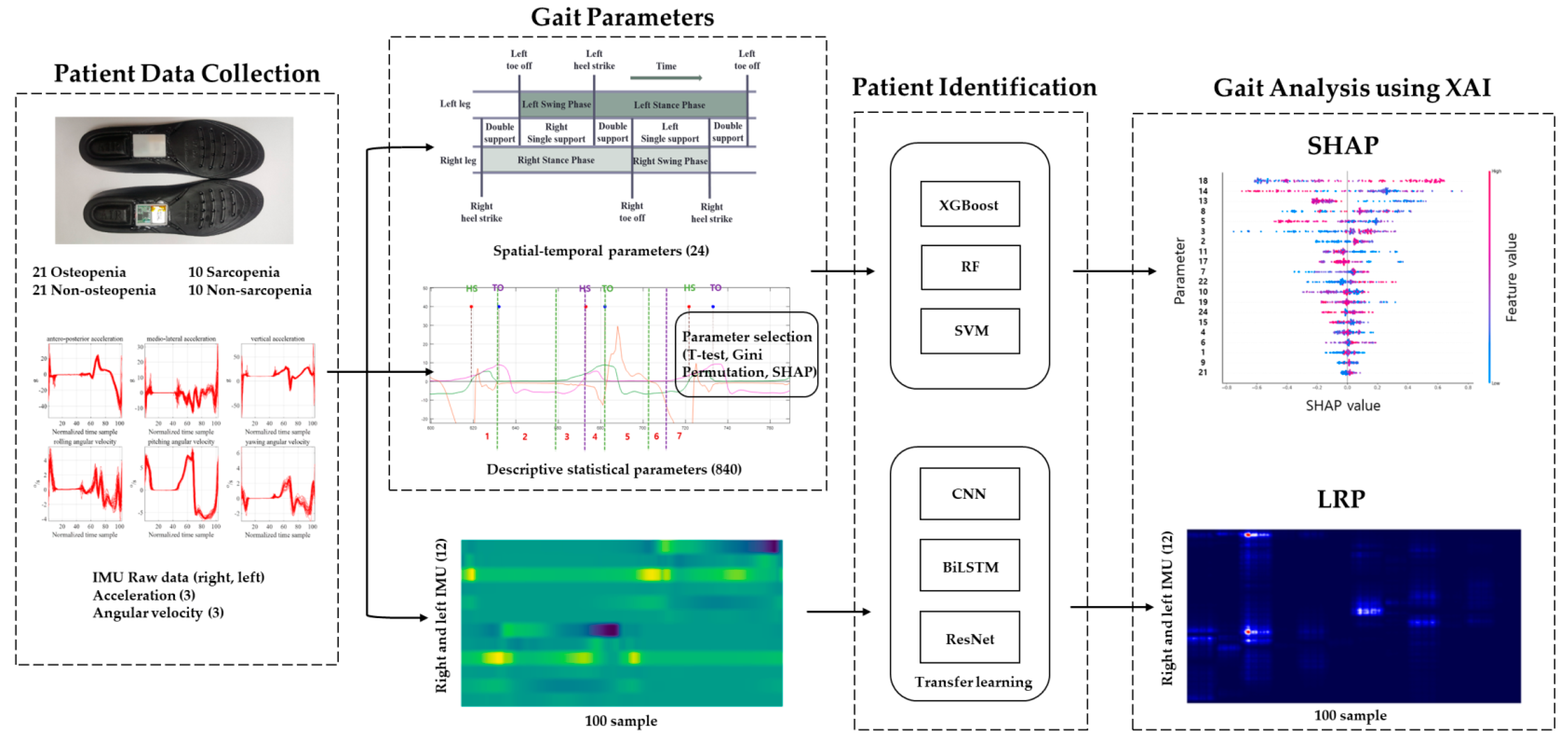
3. Methods
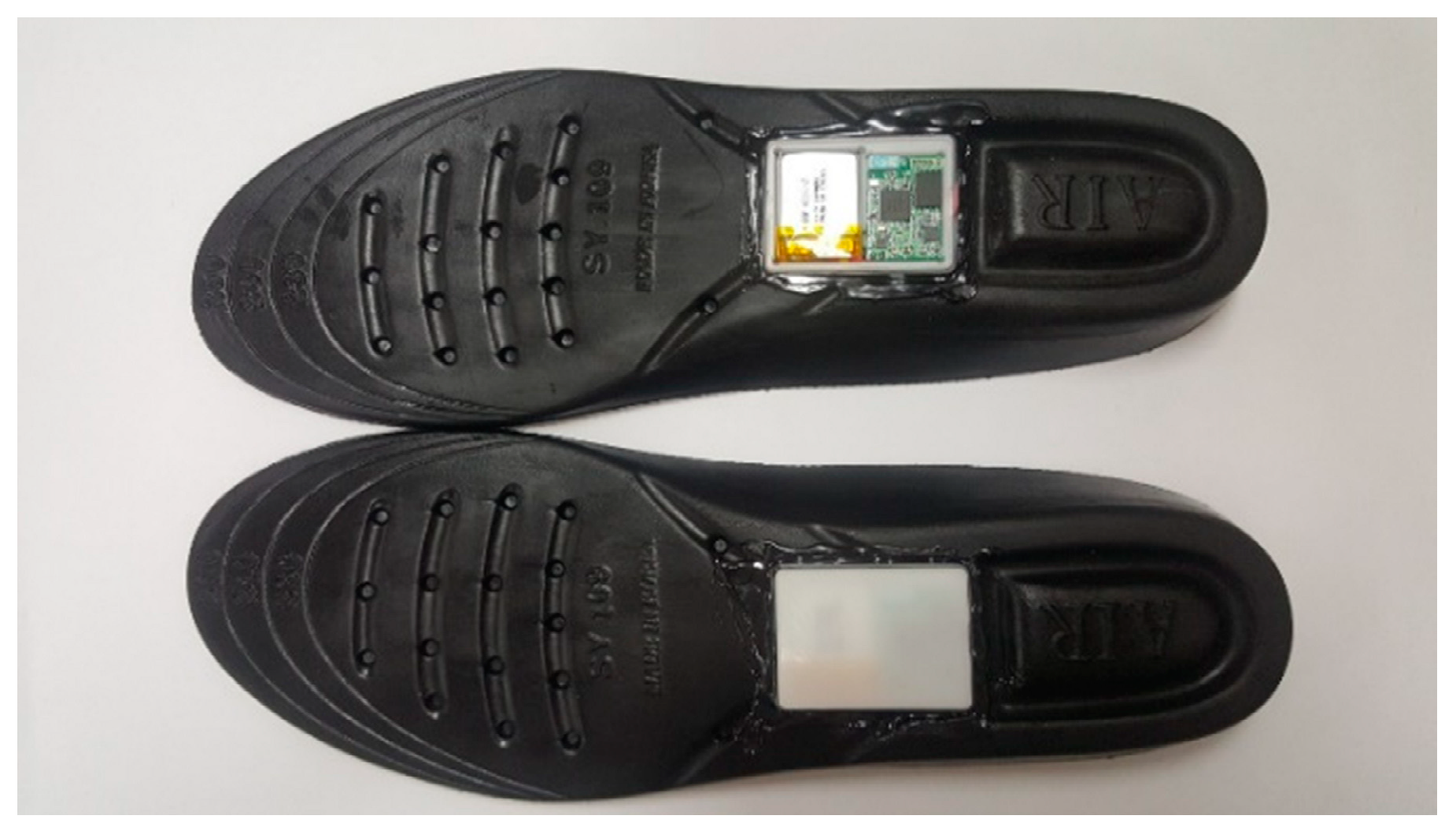
3.1. Patient Data Collection
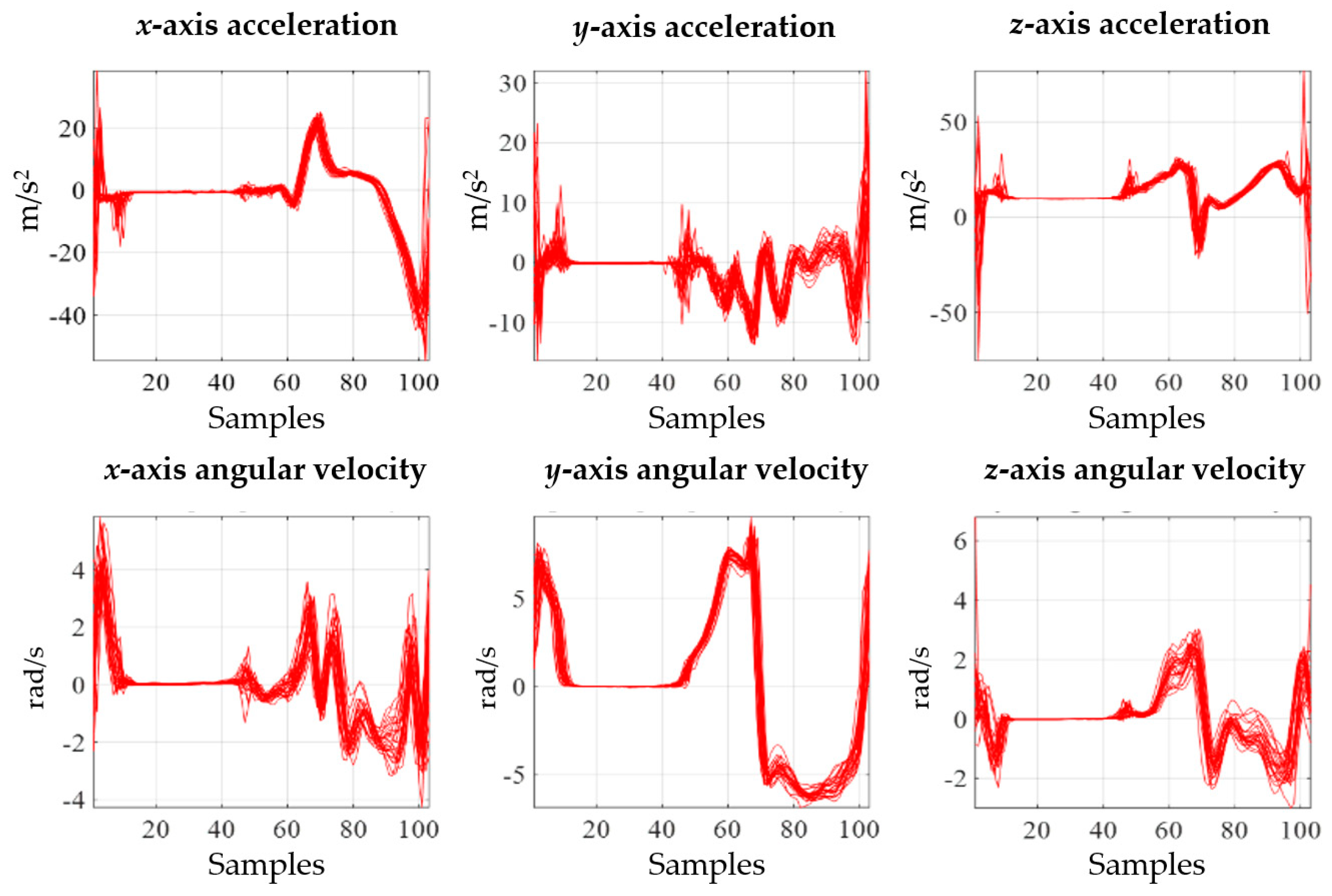
3.2. Gait Signals and Parameters
3.3. Patient Identification
3.4. Gait Analysis
4. Results
4.1. Patient Identification
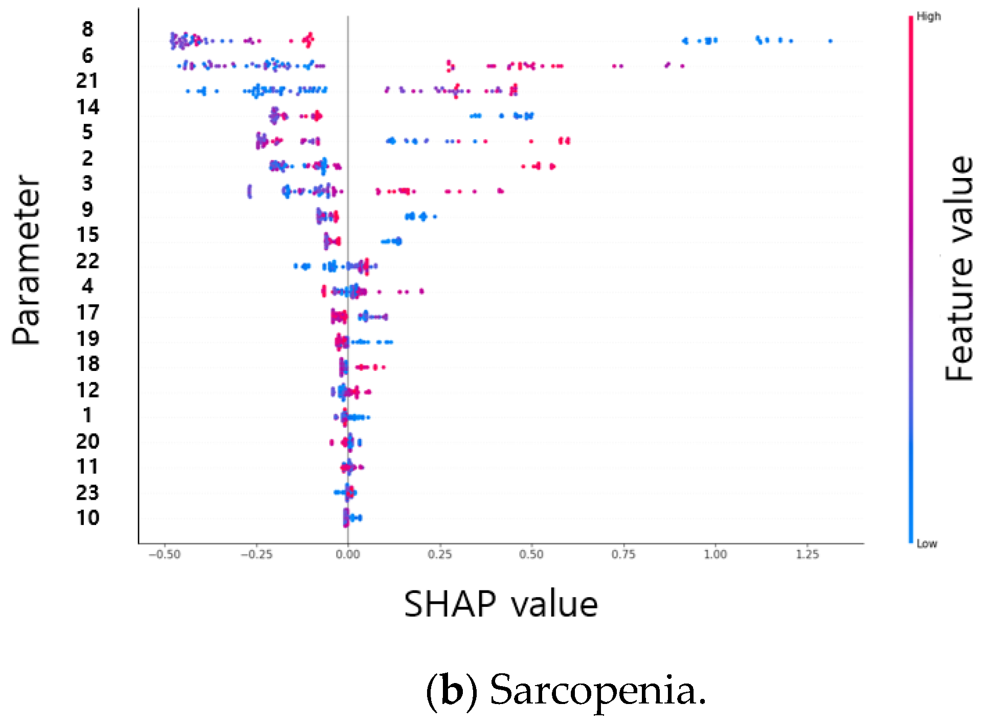
4.2. Importance of Descriptive Statistical Parameter
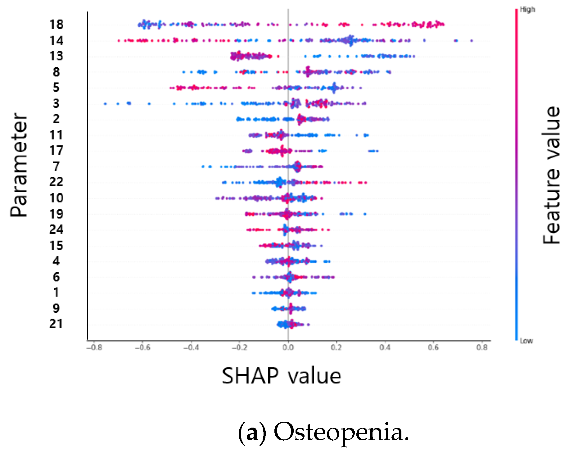
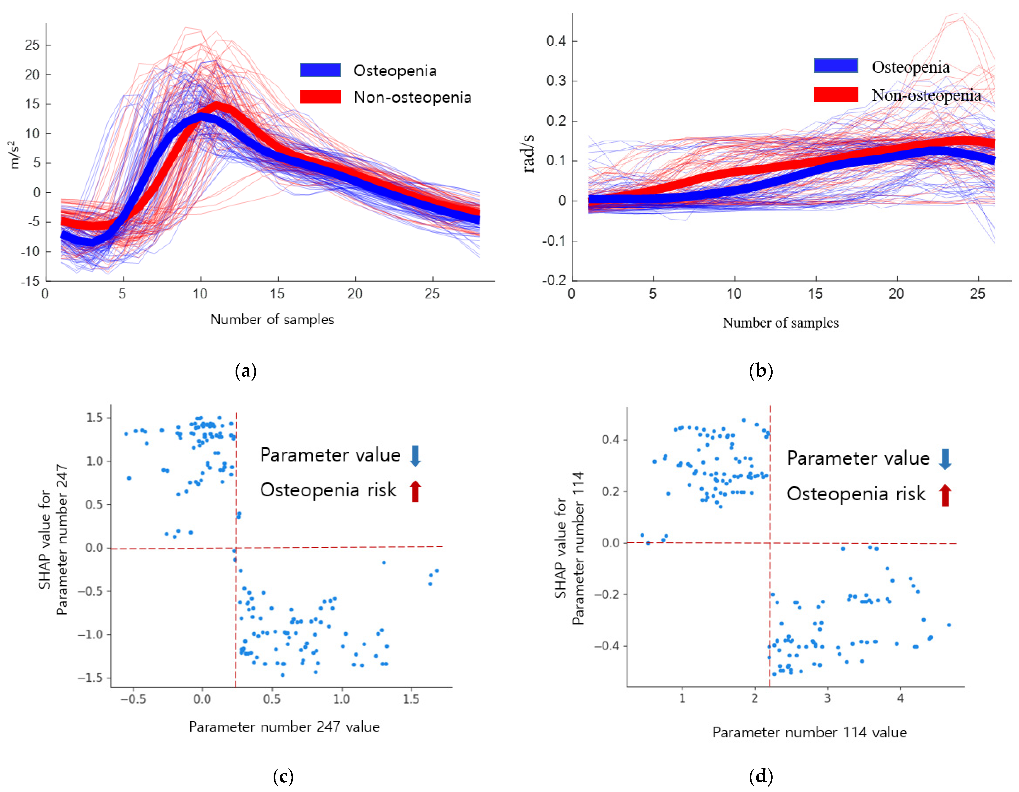
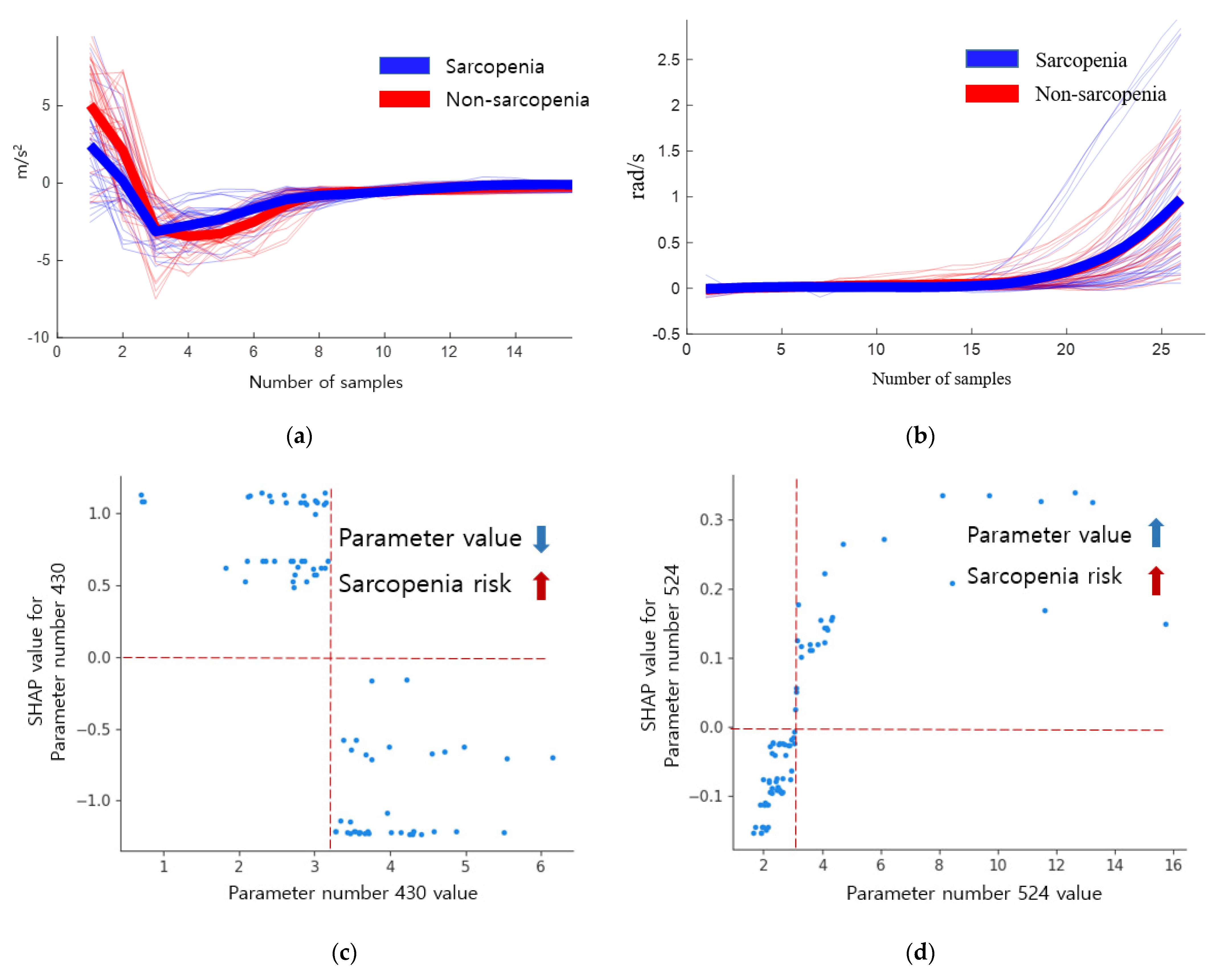
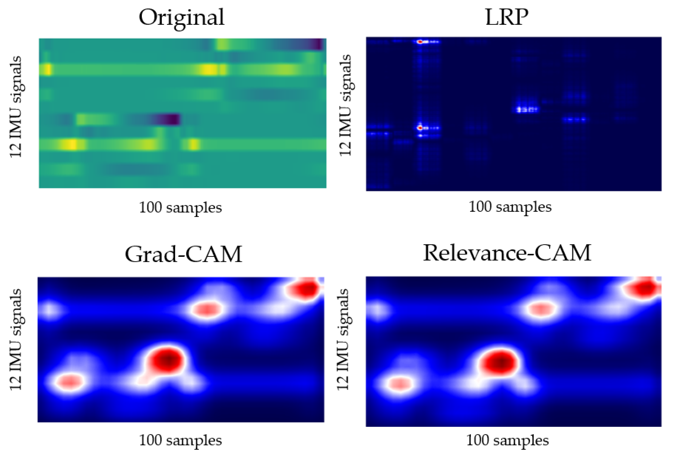
4.3. Gait Analysis
5. Discussion
6. Conclusions
Author Contributions
Funding
Institutional Review Board Statement
Informed Consent Statement
Data Availability Statement
Conflicts of Interest
Appendix A

| Abbreviations | Raw | Abbreviations | Raw |
|---|---|---|---|
| XAI | eXplainable Artificial Intelligence | LDA | Linear Discriminant Analysis |
| BMD | Bone Mineral Density | NB | Naïve Bayes |
| SD | Standard Deviation | k-NN | k-Nearest Neighbor |
| DEXA | Dual-Energy X-ray Absorptiometry | SVM | Support Vector Machines |
| PD | Parkinson’s Diseases | RBF | Radial Basis Function |
| THA | Total Hip Arthroplasty | DT | Decision Tree |
| IMU | Inertial Measurement Unit | XGBoost | Extreme Gradient Boosting |
| HS | Heel Strike | HMM | Hidden Markov Model |
| TO | Toe Off | RF | Random Forest |
| LIME | Local Interpretable Model-agnostic Explanations | ANN | Artificial Neural Network |
| SHAP | SHapley Additive exPlanations | CNN | Convolutional Neural Network |
| SMI | Skeletal Muscle mass Index | LSTM | Long Short-Term Memory |
| MMSE | Mini-Mental State Examination | ResNet | Residual neural Network |
| MFS | Mores Fall Scale | GAP | Global Average Pooling |
| TUG | Timed Up and Go | FC | Fully Connected |
| BBS | Berg Balance Scale | LRP | Layer-wise Relevance Propagation |
| ROM | Range of Motion | CAM | Class Activation Mapping |
References
- Coll, P.P.; Phu, S.; Hajjar, S.H.; Kirk, B.; Duque, G.; Taxel, P. The prevention of osteoporosis and sarcopenia in older adults. J. Am. Geriatr. Soc. 2021, 69, 1388–1398. [Google Scholar] [CrossRef] [PubMed]
- Intriago, M.; Maldonado, G.; Guerrero, R.; Messina, O.D.; Rios, C. Bone Mass Loss and Sarcopenia in Ecuadorian Patients. J. Aging Res. 2020, 2020, 1072675. [Google Scholar] [CrossRef] [PubMed][Green Version]
- Stephen, W.C.; Janssen, I. Sarcopenic-obesity and cardiovascular disease risk in the elderly. J. Nutr. Health Aging 2009, 13, 460–466. [Google Scholar] [CrossRef] [PubMed]
- Kim, J.-K.; Bae, M.-N.; Lee, K.; Hong, S. Identification of Patients with Sarcopenia Using Gait Parameters Based on Inertial Sensors. Sensors 2021, 21, 1786. [Google Scholar] [CrossRef]
- Teufl, W.; Taetz, B.; Miezal, M.; Lorenz, M.; Pietschmann, J.; Jöllenbeck, T.; Fröhlich, M.; Bleser, G. Towards an Inertial Sensor-Based Wearable Feedback System for Patients after Total Hip Arthroplasty: Validity and Applicability for Gait Classification with Gait Kinematics-Based Features. Sensors 2019, 19, 5006. [Google Scholar] [CrossRef]
- Tatangelo, G.; Watts, J.; Lim, K.; Connaughton, C.; Abimanyi-Ochom, J.; Borgström, F.; Nicholson, G.C.; Shore-Lorenti, C.; Stuart, A.L.; Iuliano-Burns, S.; et al. The cost of osteoporosis, osteopenia, and associated fractures in Australia in 2017. J. Bone Miner. Res. 2019, 34, 616–625. [Google Scholar] [CrossRef]
- Kanis, J.A. Assessment of fracture risk and its application to screening for postmenopausal osteoporosis: Synopsis of a WHO report. Osteoporos. Int. 1994, 4, 368–381. [Google Scholar] [CrossRef]
- Cruz-Jentoft, A.J.; Baeyens, J.P.; Bauer, J.M.; Boirie, Y.; Cederholm, T.; Landi, F.; Martin, F.C.; Michel, J.-P.; Rolland, Y.; Schneider, S.M. Sarcopenia: European consensus on definition and diagnosisReport of the European Working Group on Sarcopenia in Older People. Age Ageing 2010, 39, 412–423. [Google Scholar] [CrossRef]
- Caramia, C.; Torricelli, D.; Schmid, M.; Muñoz-Gonzalez, A.; Gonzalez-Vargas, J.; Grandas, F.; Pons, J.L. IMU-based classification of Parkinson’s disease from gait: A sensitivity analysis on sensor location and feature selection. IEEE J. Biomed. Health Inform. 2018, 22, 1765–1774. [Google Scholar] [CrossRef]
- Eskofier, B.M.; Lee, S.I.; Daneault, J.F.; Golabchi, F.N.; Ferreira-Carvalho, G.; Vergara-Diaz, G.; Sapienza, S.; Costante, G.; Klucken, J.; Kautz, T.; et al. Recent machine learning advancements in sensor-based mobility analysis: Deep learning for Parkinson’s disease assessment. In Proceedings of the 2016 38th Annual International Conference of the IEEE Engineering in Medicine and Biology Society (EMBC), Orlando, FL, USA, 16–20 August 2016; pp. 655–658. [Google Scholar]
- Howcroft, J.; Kofman, J.; Lemaire, E. Prospective Fall-Risk Prediction Models for Older Adults Based on Wearable Sensors. IEEE Trans. Neural Syst. Rehabil. Eng. 2017, 25, 1812–1820. [Google Scholar] [CrossRef]
- Tunca, C.; Salur, G.; Ersoy, C. Deep Learning for Fall Risk Assessment with Inertial Sensors: Utilizing Domain Knowledge in Spatio-Temporal Gait Parameters. IEEE J. Biomed. Health Inform. 2020, 24, 1994–2005. [Google Scholar] [CrossRef] [PubMed]
- Dindorf, C.; Teufl, W.; Taetz, B.; Bleser, G.; Fröhlich, M. Interpretability of Input Representations for Gait Classification in Patients after Total Hip Arthroplasty. Sensors 2020, 20, 4385. [Google Scholar] [CrossRef] [PubMed]
- Ren, L.; Peng, Y. Research of Fall Detection and Fall Prevention Technologies: A Systematic Review. IEEE Access 2019, 7, 77702–77722. [Google Scholar] [CrossRef]
- Choi, W.; Choi, J.H.; Chung, C.Y.; Sung, K.H.; Lee, K.M. Can gait kinetic data predict femoral bone mineral density in elderly men and women aged 50 years and older? J. Biomech. 2021, 123, 110520. [Google Scholar] [CrossRef] [PubMed]
- ElDeeb, A.M.; Khodair, A.S. Three-dimensional analysis of gait in postmenopausal women with low bone mineral density. J. Neuroeng. Rehabil. 2014, 11, 55. [Google Scholar] [CrossRef]
- Sung, P.S. Increased double limb support times during walking in right limb dominant healthy older adults with low bone density. Gait Posture 2018, 63, 145–149. [Google Scholar] [CrossRef]
- Gunning, D.; Aha, D. DARPA’s Explainable Artificial Intelligence (XAI) Program. AI Mag. 2019, 40, 44–58. [Google Scholar] [CrossRef]
- Parsa, A.B.; Movahedi, A.; Taghipour, H.; Derrible, S.; Mohammadian, A. (Kouros) toward safer highways, application of XGBoost and SHAP for real-time accident detection and feature analysis. Accid. Anal. Prev. 2020, 136, 105405. [Google Scholar] [CrossRef]
- Taborri, J.; Palermo, E.; Rossi, S.; Cappa, P. Gait Partitioning Methods: A Systematic Review. Sensors 2016, 16, 66. [Google Scholar] [CrossRef]
- Whittle, M.W. Gait Analysis: An Introduction; Butterworth-Heinemann: Oxford, UK, 2014. [Google Scholar]
- Kim, J.; Bae, M.-N.; Lee, K.B.; Hong, S.G. Gait event detection algorithm based on smart insoles. ETRI J. 2019, 42, 46–53. [Google Scholar] [CrossRef]
- Nilsson, J.-O.; Gupta, A.K.; Handel, P. Foot-mounted inertial navigation made easy. In Proceedings of the 2014 International Conference on Indoor Positioning and Indoor Navigation (IPIN), Busan, Korea, 27–30 October 2014; pp. 24–29. [Google Scholar]
- Skog, I.; Nilsson, J.-O.; Handel, P. Pedestrian tracking using an IMU array. In Proceedings of the 2014 IEEE International Conference on Electronics, Computing and Communication Technologies (CONECCT), Bangalore, India, 6–7 January 2014; pp. 1–4. [Google Scholar]
- Bach, S.; Binder, A.; Montavon, G.; Klauschen, F.; Müller, K.-R.; Samek, W. On Pixel-Wise Explanations for Non-Linear Classifier Decisions by Layer-Wise Relevance Propagation. PLoS ONE 2015, 10, e0130140. [Google Scholar] [CrossRef] [PubMed]
- Zhou, B.; Khosla, A.; Lapedriza, A.; Oliva, A.; Torralba, A. Learning deep features for discriminative localization. In Proceedings of the IEEE Conference on Computer Vision and Pattern Recognition, Las Vegas, NV, USA, 27–30 June 2016; pp. 2921–2929. [Google Scholar]
- Lee, J.R.; Kim, S.; Park, I.; Eo, T.; Hwang, D. Relevance-CAM: Your Model Already Knows Where to Look. In Proceedings of the 2021 IEEE/CVF Conference on Computer Vision and Pattern Recognition (CVPR), Nashville, TN, USA, 20–25 June 2021; pp. 14939–14948. [Google Scholar]
- Kang, Y.; Na, D.L.; Hahn, S. A validity study on the Korean Mini-Mental State Examination (K-MMSE) in dementia patients. J. Korean Neurol. Assoc. 1997, 15, 300–308. [Google Scholar]
- Baek, S.; Piao, J.; Jin, Y.J.; Lee, S.-M. Validity of the Morse Fall Scale implemented in an electronic medical record system. J. Clin. Nurs. 2014, 23, 2434–2441. [Google Scholar] [CrossRef] [PubMed]
- Kim, S.; Kim, M.; Won, C.W. Validation of the Korean version of the SARC-F questionnaire to assess sarcopenia: Korean frailty and aging cohort study. J. Am. Med. Dir. Assoc. 2018, 19, 40–45. [Google Scholar] [CrossRef]
- Berg, K.; Wood-Dauphine, S.; Williams, J.I.; Gayton, D. Measuring balance in the elderly: Preliminary development of an instrument. Physiother. Can. 1989, 41, 304–311. [Google Scholar] [CrossRef]
- Podsiadlo, D.; Richardson, S. The timed “Up & Go”: A test of basic functional mobility for frail elderly persons. J. Am. Geriatr. Soc. 1991, 39, 142–148. [Google Scholar]
- Zhang, D.; Qian, L.; Mao, B.; Huang, C.; Huang, B.; Si, Y. A Data-Driven Design for Fault Detection of Wind Turbines Using Random Forests and XGboost. IEEE Access 2018, 6, 21020–21031. [Google Scholar] [CrossRef]
- Duan, H.; Zhao, Y.; Chen, K.; Shao, D.; Lin, D.; Dai, B. Revisiting Skeleton-based Action Recognition. arXiv 2021, arXiv:2104.13586. [Google Scholar]
- Wu, Z.; Shen, C.; Van Den Hengel, A. Wider or deeper: Revisiting the resnet model for visual recognition. Pattern Recog. 2019, 90, 119–133. [Google Scholar] [CrossRef]
- Wan, Z.; Yang, R.; Huang, M.; Zeng, N.; Liu, X. A review on transfer learning in EEG signal analysis. Neurocomputing 2021, 421, 1–14. [Google Scholar] [CrossRef]


| Reference | Parameter | Disease | Position | Classification | Accuracy |
|---|---|---|---|---|---|
| Caramia 2018 [9] | Step length, step time, stride time, speed, hip, knee, and ankle ROM | PD | R and L ankle, knee, hip, chest | LDA, NB, k-NN, SVM, SVM RBF, DT, majority of votes | 96.88% |
| Eskofier 2016 [10] | Energy maximum, minimum, mean, variance, skewness, kurtosis, fast Fourier transform | PD | Upper limbs | AdaBoost, PART, k-NN, SVM, CNN | 90.9% |
| Howcroft 2017 [11] | Cadence, stride time maximum, mean, and SD of acceleration | Faller | Head, pelvis, R and L shank | NB, SVM, NN | 57% |
| Tunca 2019 [12] | Stride length, cycle time, stance time, swing time, clearance, stance ratio, cadence, speed | Faller | Both feet | SVM, RF, MLP, HMM, LSTM | 94.30% |
| Teufl 2019 [5] | Stride length, stride time, cadence, speed, hip and pelvis ROM | THA | Hip, thigh, shank, foot | SVM | 97% |
| Dindorf 2020 [13] | Various parameters | THA | Hip, knee, pelvis, ankle | RF, SVM, SVM RBF, MLP | 100% |
| Kim 2021 [4] | Various parameters | Sarcopenia | Both feet | RF, SVM, MLP, CNN, BiLSTM | 95% |
| Ours | Various parameters | Osteopenia Sarcopenia | Both feet | RF, SVM, XGBoost, CNN, BiLSTM, ResNet | 88.69% 93.75% |
| Parameter | Osteopenia | Non-Osteopenia | Osteopenia p-Value | Sarcopenia | Non-Sarcopenia | Sarcopenia p-Value |
|---|---|---|---|---|---|---|
| Age (years) | 70.48 ± 2.36 | 70.33 ± 2.56 | 0.852 | 71.10 ± 2.13 | 69.50 ± 3.14 | 0.199 |
| Height (cm) | 153.65 ± 4.83 | 152.80 ± 5.93 | 0.614 | 150.87 ± 4.66 | 153.10 ± 4.36 | 0.283 |
| Weight (kg) | 57.75 ± 6.12 | 59.57 ± 7.12 | 0.379 | 53.55 ± 5.62 | 61.20 ± 5.07 | 0.005 |
| Feet_size (mm) | 236.91 ± 7.66 | 238.57 ± 6.55 | 0.453 | 232.00 ± 5.87 | 239.50 ± 6.43 | 0.014 |
| MMSE | 27.62 ± 1.77 | 28.19 ± 1.78 | 0.303 | 27.80 ± 1.40 | 27.30 ± 2.16 | 0.547 |
| SARC-F | 3.19 ± 2.40 | 3.86 ± 2.15 | 0.349 | 2.90 ± 1.52 | 2.90 ± 2.85 | 1.000 |
| MFS | 23.10±17.92 | 26.43 ± 16.59 | 0.535 | 13.50 ± 12.92 | 23.50 ± 12.70 | 0.098 |
| BBS | 42.38 ± 8.48 | 42.19 ± 6.85 | 0.937 | 43.10 ± 6.26 | 41.90 ± 9.47 | 0.742 |
| 3m TUG | 10.96 ± 1.64 | 11.50 ± 2.87 | 0.464 | 11.71 ± 1.62 | 9.85 ± 1.92 | 0.031 |
| Grasp_right (kg) | 17.29 ± 5.42 | 18.77 ± 4.71 | 0.351 | 14.42 ± 3.65 | 22.57 ± 2.73 | 0.000 |
| Grasp_left (kg) | 17.61 ± 4.67 | 18.04 ± 4.40 | 0.761 | 14.15 ± 3.97 | 22.17 ± 3.02 | 0.000 |
| T_score (DEXA) | −1.85 ± 0.74 | 0.69 ± 1.49 | 0.000 | −0.49 ± 2.08 | −0.64 ± 2.03 | 0.872 |
| SMI(ASM/height) | 5.37 ± 0.55 | 5.38 ± 0.65 | 0.961 | 4.58 ± 0.32 | 5.93 ± 0.35 | 0.000 |
| Gait Parameters | Definition |
|---|---|
| Spatial–temporal parameters | |
| Cadence | Number of steps acquired per minute |
| Stance phase (time) | Percent (time) starting with HS and ending with TO of the same foot |
| Swing phase (time) | Percent (time) starting with TO and ending with HS of the same foot |
| Single support phase (time) | Percent (time) when only one foot is on the ground |
| Double support phase (time) | Percent (time) when both feet are on the ground |
| Stride length | Distance starting with HS and ending with next HS of the same foot |
| Symmetry indices (SI) | Absolute values of (right—left)/(0.5 × ( right + left ) |
| Descriptive statistical parameters | |
| Max | Greatest values |
| Min | Least or smallest values |
| SD | Standard deviation of values |
| AbSum | Absolute sum of values |
| Root-mean-square (RMS) | Arithmetic mean of the squares of a set of values |
| Kurtosis | Assesses whether the tails of a given distribution contain extreme values |
| Skewness | A measure of the asymmetry of the probability distribution of a real-valued random variable about its mean |
| MMgr | Gradient from maximum value to minimum value |
| DMM | Difference between maximum value and minimum value |
| Mdif | Maximum for the difference between two successive values |
| CNN | BiLSTM | ResNet50 | |||
|---|---|---|---|---|---|
| Input | None, 100, 36, 1 | Input | None, 100, 36, 1 | Input | None, 100, 36, 1 |
| Conv1 | , 5 max pooling, | BiLSTM1 | 5 | Conv1 | , 64 stride 2 max pooling, stride 2 |
| Conv2 | , 5 max pooling, | BiLSTM2 | 10 | Conv2 | |
| Conv3 | 3, 20 | Dropout | 0.5 | Conv3 | |
| Dropout | 0.5 | FC, Dense | Conv4 | ||
| FC, Dense | Conv5 | ||||
| GAP, FC | |||||
| Groups | Parameters | Models | Accuracy | Precision | Recall | F1-Score |
|---|---|---|---|---|---|---|
| Osteopenia | Spatial–temporal (24) | RF | 0.494 | 0.476 | 0.370 | 0.393 |
| XGBoost | 0.476 | 0.476 | 0.376 | 0.406 | ||
| SVM | 0.637 | 0.619 | 0.511 | 0.544 | ||
| Descriptive statistical (100) | RF | 0.649 | 0.655 | 0.612 | 0.607 | |
| XGBoost | 0.684 | 0.690 | 0.680 | 0.650 | ||
| SVM | 0.607 | 0.678 | 0.590 | 0.604 | ||
| Sarcopenia | Spatial–temporal (24) | RF | 0.802 | 0.825 | 0.775 | 0.775 |
| XGBoost | 0.752 | 0.725 | 0.667 | 0.677 | ||
| SVM | 0.775 | 0.603 | 0.775 | 0.658 | ||
| Descriptive statistical (100) | RF | 0.675 | 0.675 | 0.632 | 0.631 | |
| XGBoost | 0.603 | 0.675 | 0.557 | 0.591 | ||
| SVM | 0.637 | 0.704 | 0.657 | 0.644 |
| Groups | Models | Accuracy | Precision | Recall | F1-Score |
|---|---|---|---|---|---|
| Osteopenia | CNN | 0.696 | 0.690 | 0.735 | 0.670 |
| BiLSTM | 0.619 | 0.570 | 0.610 | 0.571 | |
| ResNet | 0.767 | 0.672 | 0.726 | 0.676 | |
| ResNet(transfer) | 0.786 | 0.869 | 0.747 | 0.787 | |
| Sarcopenia | CNN | 0.600 | 0.437 | 0.525 | 0.447 |
| BiLSTM | 0.425 | 0.300 | 0.350 | 0.299 | |
| ResNet | 0.612 | 0.337 | 0.500 | 0.394 | |
| ResNet(transfer) | 0.700 | 0.612 | 0.636 | 0.606 |
| Class | ML | Number of Parameters | ||||||||||
|---|---|---|---|---|---|---|---|---|---|---|---|---|
| 2 | 3 | 4 | 5 | 6 | 7 | 8 | 9 | 10 | 20 | 100 | ||
| Gini | RF | 70.83 | 70.23 | 64.88 | 72.02 | 68.45 | 63.69 | 61.30 | 60.11 | 60.71 | 61.30 | 64.88 |
| XGBoost | 66.66 | 67.85 | 64.88 | 71.42 | 68.45 | 64.28 | 65.47 | 61.30 | 65.47 | 67.26 | 68.45 | |
| SVM | 64.28 | 64.88 | 64.88 | 64.28 | 61.30 | 61.30 | 59.52 | 55.35 | 57.73 | 58.33 | 60.71 | |
| Permutation | RF | 73.21 | 70.83 | 69.64 | 67.26 | 64.28 | 68.45 | 70.23 | 69.04 | 67.26 | 67.26 | 64.88 |
| XGBoost | 69.64 | 70.83 | 70.23 | 68.42 | 64.88 | 65.47 | 67.26 | 66.70 | 67.26 | 70.23 | 68.45 | |
| SVM | 65.47 | 68.45 | 66.07 | 64.28 | 66.66 | 66.66 | 64.28 | 64.88 | 64.88 | 60.71 | 60.71 | |
| SHAP | RF | 73.80 | 76.19 | 70.23 | 63.69 | 63.09 | 63.69 | 63.09 | 63.69 | 57.73 | 60.11 | 64.88 |
| XGBoost | 70.23 | 75 | 74.40 | 73.21 | 66.66 | 67.85 | 63.69 | 59.52 | 56.54 | 68.45 | 68.45 | |
| SVM | 71.42 | 71.42 | 67.26 | 61.30 | 58.33 | 58.33 | 57.14 | 55.95 | 57.14 | 62.5 | 60.71 | |
| Class | ML | Number of Parameters | ||||||||||
|---|---|---|---|---|---|---|---|---|---|---|---|---|
| 2 | 3 | 4 | 5 | 10 | 15 | 16 | 17 | 18 | 20 | 100 | ||
| Gini | RF | 50 | 58.75 | 62.5 | 65 | 68.75 | 67.5 | 68.75 | 71.25 | 71.25 | 62.5 | 67.5 |
| XGBoost | 52.5 | 57.5 | 65 | 66.25 | 62.5 | 58.75 | 58.75 | 58.75 | 58.75 | 58.75 | 60 | |
| SVM | 52.5 | 58.75 | 66.25 | 65 | 72.5 | 57.5 | 56.25 | 56.25 | 58.75 | 60 | 63.75 | |
| Permutation | RF | 62.5 | 60 | 56.25 | 53.75 | 57.5 | 67.5 | 55 | 60 | 70 | 62.5 | 67.5 |
| XGBoost | 60 | 60 | 55 | 58.75 | 65 | 63.75 | 68.75 | 65 | 66.25 | 67.5 | 60 | |
| SVM | 61.25 | 60 | 60 | 55 | 65 | 66.25 | 66.25 | 68.75 | 63.75 | 60 | 63.75 | |
| SHAP | RF | 56.25 | 60 | 57.5 | 65 | 67.5 | 62.5 | 72.5 | 73.75 | 68.75 | 67.5 | 67.5 |
| XGBoost | 46.25 | 63.75 | 62.5 | 65 | 65 | 63.75 | 63.75 | 65 | 66.25 | 63.75 | 60 | |
| SVM | 58.75 | 67.5 | 60 | 61.25 | 675 | 66.25 | 68.75 | 62.5 | 60 | 58.75 | 63.75 | |
| Class | Important Parameter | 1 | 2 | 3 | 4 | 5 | 6 | 7 | 8 | 9 | 10 |
| Osteopenia | Parameters | 247 | 114 | 87 | 218 | 816 | 206 | 291 | 21 | 169 | 667 |
| Shapley value | 0.97 | 0.28 | 0.27 | 0.2 | 0.18 | 0.17 | 0.16 | 0.13 | 0.1 | 0.09 | |
| Sarcopenia | Parameters | 430 | 524 | 51 | 9 | 270 | 457 | 231 | 387 | 3 | 97 |
| Shapley value | 0.66 | 0.28 | 0.25 | 0.22 | 0.17 | 0.16 | 0.15 | 0.13 | 0.13 | 0.13 | |
| Class | Important Parameter | 11 | 12 | 13 | 14 | 15 | 16 | 17 | 18 | 19 | 20 |
| Osteopenia | Parameters | 774 | 117 | 45 | 802 | 312 | 23 | 542 | 242 | 554 | 422 |
| Shapley value | 0.09 | 0.08 | 0.08 | 0.07 | 0.07 | 0.07 | 0.07 | 0.06 | 0.06 | 0.06 | |
| Sarcopenia | Parameters | 5 | 67 | 521 | 690 | 607 | 704 | 380 | 469 | 8 | 257 |
| Shapley value | 0.13 | 0.12 | 0.11 | 0.09 | 0.09 | 0.08 | 0.08 | 0.08 | 0.08 | 0.07 |
| Right | Left | ||||||||||||||||||||
|---|---|---|---|---|---|---|---|---|---|---|---|---|---|---|---|---|---|---|---|---|---|
| Parameter | Max | Min | SD | AbSum | RMS | Ku | Ske | MMgr | DMM | Mdif | Max | Min | SD | AbSum | RMS | Ku | Ske | MMgr | DMM | Mdif | |
| Loading response | AccX | 1 | 2 | 3 | 4 | 5 | 6 | 7 | 8 | 9 | 10 | 421 | 422 | 423 | 424 | 425 | 426 | 427 | 428 | 429 | 430 |
| AccY | 11 | 12 | 13 | 14 | 15 | 16 | 17 | 18 | 19 | 20 | 431 | 432 | 433 | 434 | 435 | 436 | 437 | 438 | 439 | 440 | |
| AccZ | 21 | 22 | 23 | 24 | 25 | 26 | 27 | 28 | 29 | 30 | 441 | 442 | 443 | 444 | 445 | 446 | 447 | 448 | 449 | 450 | |
| GyroX | 31 | 32 | 33 | 34 | 35 | 36 | 37 | 38 | 39 | 40 | 451 | 452 | 453 | 454 | 455 | 456 | 457 | 458 | 459 | 460 | |
| GyroY | 41 | 42 | 43 | 44 | 45 | 46 | 47 | 48 | 49 | 50 | 461 | 462 | 463 | 464 | 465 | 466 | 467 | 468 | 469 | 470 | |
| GyroZ | 51 | 52 | 53 | 54 | 55 | 56 | 57 | 58 | 59 | 60 | 471 | 472 | 473 | 474 | 475 | 476 | 477 | 478 | 479 | 480 | |
| Mid stance | AccX | 61 | 62 | 63 | 64 | 65 | 66 | 67 | 68 | 69 | 70 | 481 | 482 | 483 | 484 | 485 | 486 | 487 | 488 | 489 | 490 |
| AccY | 71 | 72 | 73 | 74 | 75 | 76 | 77 | 78 | 79 | 80 | 491 | 492 | 493 | 494 | 495 | 496 | 497 | 498 | 499 | 500 | |
| AccZ | 81 | 82 | 83 | 84 | 85 | 86 | 87 | 88 | 89 | 90 | 501 | 502 | 503 | 504 | 505 | 506 | 507 | 508 | 509 | 510 | |
| GyroX | 91 | 92 | 93 | 94 | 95 | 96 | 97 | 98 | 99 | 100 | 511 | 512 | 513 | 514 | 515 | 516 | 517 | 518 | 519 | 520 | |
| GyroY | 101 | 102 | 103 | 104 | 105 | 106 | 107 | 108 | 109 | 110 | 521 | 522 | 523 | 524 | 525 | 526 | 527 | 528 | 529 | 530 | |
| GyroZ | 111 | 112 | 113 | 114 | 115 | 116 | 117 | 118 | 119 | 120 | 531 | 532 | 533 | 534 | 535 | 536 | 537 | 538 | 539 | 540 | |
| Terminal stance | AccX | 121 | 122 | 123 | 124 | 125 | 126 | 127 | 128 | 129 | 130 | 541 | 542 | 543 | 544 | 545 | 546 | 547 | 548 | 549 | 550 |
| AccY | 131 | 132 | 133 | 134 | 135 | 136 | 137 | 138 | 139 | 140 | 551 | 552 | 553 | 554 | 555 | 556 | 557 | 558 | 559 | 560 | |
| AccZ | 141 | 142 | 143 | 144 | 145 | 146 | 147 | 148 | 149 | 150 | 561 | 562 | 563 | 564 | 565 | 566 | 567 | 568 | 569 | 570 | |
| GyroX | 151 | 152 | 153 | 154 | 155 | 156 | 157 | 158 | 159 | 160 | 571 | 572 | 573 | 574 | 575 | 576 | 577 | 578 | 579 | 580 | |
| GyroY | 161 | 162 | 163 | 164 | 165 | 166 | 167 | 168 | 169 | 170 | 581 | 582 | 583 | 584 | 585 | 586 | 587 | 588 | 589 | 590 | |
| GyroZ | 171 | 172 | 173 | 174 | 175 | 176 | 177 | 178 | 179 | 180 | 591 | 592 | 593 | 594 | 595 | 596 | 597 | 598 | 599 | 600 | |
| Pre swing | AccX | 181 | 182 | 183 | 184 | 185 | 186 | 187 | 188 | 189 | 190 | 601 | 602 | 603 | 604 | 605 | 606 | 607 | 608 | 609 | 610 |
| AccY | 191 | 192 | 193 | 194 | 195 | 196 | 197 | 198 | 199 | 200 | 611 | 612 | 613 | 614 | 615 | 616 | 617 | 618 | 619 | 620 | |
| AccZ | 201 | 202 | 203 | 204 | 205 | 206 | 207 | 208 | 209 | 210 | 621 | 622 | 623 | 624 | 625 | 626 | 627 | 628 | 629 | 630 | |
| GyroX | 211 | 212 | 213 | 214 | 215 | 216 | 217 | 218 | 219 | 220 | 631 | 632 | 633 | 634 | 635 | 636 | 637 | 638 | 639 | 640 | |
| GyroY | 221 | 222 | 223 | 224 | 225 | 226 | 227 | 228 | 229 | 230 | 641 | 642 | 643 | 644 | 645 | 646 | 647 | 648 | 649 | 650 | |
| GyroZ | 231 | 232 | 233 | 234 | 235 | 236 | 237 | 238 | 239 | 240 | 651 | 652 | 653 | 654 | 655 | 656 | 657 | 658 | 659 | 660 | |
| Initial swing | AccX | 241 | 242 | 243 | 244 | 245 | 246 | 247 | 248 | 249 | 250 | 661 | 662 | 663 | 664 | 665 | 666 | 667 | 668 | 669 | 670 |
| AccY | 251 | 252 | 253 | 254 | 255 | 256 | 257 | 258 | 259 | 260 | 671 | 672 | 673 | 674 | 675 | 676 | 677 | 678 | 679 | 680 | |
| AccZ | 261 | 262 | 263 | 264 | 265 | 266 | 267 | 268 | 269 | 270 | 681 | 682 | 683 | 684 | 685 | 686 | 687 | 688 | 689 | 690 | |
| GyroX | 271 | 272 | 273 | 274 | 275 | 276 | 277 | 278 | 279 | 280 | 691 | 692 | 693 | 694 | 695 | 696 | 697 | 698 | 699 | 700 | |
| GyroY | 281 | 282 | 283 | 284 | 285 | 286 | 287 | 288 | 289 | 290 | 701 | 702 | 703 | 704 | 705 | 706 | 707 | 708 | 709 | 710 | |
| GyroZ | 291 | 292 | 293 | 294 | 295 | 296 | 297 | 298 | 299 | 300 | 711 | 712 | 713 | 714 | 715 | 716 | 717 | 718 | 719 | 720 | |
| Mid swing | AccX | 301 | 30 | 303 | 304 | 305 | 306 | 307 | 308 | 309 | 310 | 721 | 722 | 723 | 724 | 725 | 726 | 727 | 728 | 729 | 730 |
| AccY | 311 | 312 | 313 | 314 | 315 | 316 | 317 | 318 | 319 | 320 | 731 | 732 | 733 | 734 | 735 | 736 | 737 | 738 | 739 | 740 | |
| AccZ | 321 | 322 | 323 | 324 | 325 | 326 | 327 | 328 | 329 | 330 | 741 | 742 | 743 | 744 | 745 | 746 | 747 | 748 | 749 | 750 | |
| GyroX | 331 | 332 | 333 | 334 | 335 | 336 | 337 | 338 | 339 | 340 | 751 | 752 | 753 | 754 | 755 | 756 | 757 | 758 | 759 | 760 | |
| GyroY | 341 | 342 | 343 | 344 | 345 | 346 | 347 | 348 | 349 | 350 | 761 | 762 | 763 | 764 | 765 | 766 | 767 | 768 | 769 | 770 | |
| GyroZ | 351 | 352 | 353 | 354 | 355 | 356 | 357 | 358 | 359 | 360 | 771 | 772 | 773 | 774 | 775 | 776 | 777 | 778 | 779 | 780 | |
| Terminal swing | AccX | 361 | 362 | 363 | 364 | 365 | 366 | 367 | 368 | 369 | 370 | 781 | 782 | 783 | 784 | 785 | 786 | 787 | 788 | 789 | 790 |
| AccY | 371 | 372 | 373 | 374 | 375 | 376 | 377 | 378 | 379 | 380 | 791 | 792 | 793 | 794 | 795 | 796 | 797 | 798 | 799 | 800 | |
| AccZ | 381 | 382 | 383 | 384 | 385 | 386 | 387 | 388 | 389 | 390 | 801 | 802 | 803 | 804 | 805 | 806 | 807 | 808 | 809 | 810 | |
| GyroX | 391 | 392 | 393 | 394 | 395 | 396 | 397 | 398 | 399 | 400 | 811 | 812 | 813 | 814 | 815 | 816 | 817 | 818 | 819 | 820 | |
| GyroY | 401 | 402 | 403 | 404 | 405 | 406 | 407 | 408 | 409 | 410 | 821 | 822 | 823 | 824 | 825 | 826 | 827 | 828 | 829 | 830 | |
| GyroZ | 411 | 412 | 413 | 414 | 415 | 416 | 417 | 418 | 419 | 420 | 831 | 832 | 833 | 834 | 835 | 836 | 837 | 838 | 839 | 840 | |
| Class | Important Parameter | 1 | 2 | 3 | 4 | 5 | 6 | 7 | 8 | 9 | 10 |
| Osteopenia | RF | x | 75 | 85.11 | 85.71 | 78.57 | 82.14 | 80.95 | 81.54 | 77.97 | 76.78 |
| XGBoost | x | 72.02 | 80.95 | 88.69 | 87.69 | 87.5 | 85.11 | 82.73 | 81.54 | 83.33 | |
| SVM | x | 74.40 | 75 | 75.59 | 83.92 | 82.73 | 80.95 | 81.54 | 80.35 | 78.57 | |
| Sarcopenia | RF | x | 85 | 82.5 | 83.75 | 85 | 85 | 86.25 | 82.5 | 8 | 82.5 |
| XGBoost | x | 80 | 72.5 | 78.75 | 76.25 | 73.75 | 75 | 71.25 | 73.75 | 71.25 | |
| SVM | x | 81.25 | 80 | 82.5 | 81.25 | 82.5 | 86.25 | 86.25 | 87.5 | 81.25 | |
| Class | Important Parameter | 11 | 12 | 13 | 14 | 15 | 16 | 17 | 18 | 19 | 20 |
| Osteopenia | RF | 77.38 | 72.61 | 78.57 | 74.40 | 79.16 | 82.14 | 79.76 | 73.80 | 82.14 | 82.73 |
| XGBoost | 76.78 | 76.78 | 76.19 | 77.97 | 80.95 | 81.54 | 77.38 | 74.40 | 73.80 | 74.40 | |
| SVM | 76.19 | 77.97 | 74.40 | 72.61 | 75.59 | 76.78 | 76.19 | 77.97 | 79.16 | 74.40 | |
| Sarcopenia | RF | 81.25 | 83.75 | 86.25 | 88.75 | 86.25 | 87.5 | 91.25 | 93.75 | 86.25 | 92.5 |
| XGBoost | 71.52 | 75 | 71.25 | 70 | 71.25 | 75. | 72.5 | 72.5 | 71.25 | 72.5 | |
| SVM | 80 | 83.75 | 86.25 | 83.75 | 86.25 | 81.25 | 83.75 | 78.75 | 78.75 | 78.75 |
| Parameter | Osteopenia | Non-Osteopenia | Shapley Value | Sarcopenia | Non-Sarcopenia | Shapley Value | |
|---|---|---|---|---|---|---|---|
| 1 | Stance phase time right (s) | 0.61 | 0.645 | 0.034 ** | 0.614 | 0.608 | 0.014 |
| 2 | Stance phase time left (s) | 0.612 | 0.641 | 0.084 * | 0.617 | 0.604 | 0.18 |
| 3 | Swing phase time right (s) | 0.427 | 0.419 | 0.156 | 0.416 | 0.414 | 0.143 |
| 4 | Swing phase time left (s) | 0.424 | 0.422 | 0.04 | 0.412 | 0.417 | 0.039 |
| 5 | Stance phase percent right (%) | 58.77 | 60.442 | 0.196 ** | 59.468 | 59.445 | 0.235 |
| 6 | Stance phase percent left (%) | 59.05 | 60.124 | 0.035 ** | 59.853 | 59.114 | 0.345 |
| 7 | Double support first phase time right (s) | 0.1 | 0.115 | 0.074 ** | 0.112 | 0.099 | 0.005 |
| 8 | Double support first phase time left (s) | 0.085 | 0.106 | 0.197 ** | 0.09 | 0.090 | 0.551 |
| 9 | Double support second phase time right (s) | 0.085 | 0.106 | 0.031 ** | 0.09 | 0.090 | 0.097 |
| 10 | Double support second phase time left (s) | 0.1 | 0.115 | 0.072 ** | 0.111 | 0.099 | 0.007 |
| 11 | Single support phase time right (s) | 0.424 | 0.422 | 0.078 | 0.412 | 0.418 | 0.007 |
| 12 | Single support phase time left (s) | 0.427 | 0.419 | 0.017 | 0.416 | 0.414 | 0.018 |
| 13 | Double support first phase percent right (%) | 9.66 | 10.711 | 0.224 | 10.802 | 9.692 | 0 |
| 14 | Double support first phase percent left (%) | 8.18 | 9.857 | 0.311 ** | 8.563 | 8.858 | 0.248 |
| 15 | Double support second phase percent right (%) | 8.17 | 9.846 | 0.046 ** | 8.556 | 8.855 | 0.072 |
| 16 | Double support second phase percent left (%) | 9.606 | 10.686 | 0.017 ** | 10.727 | 9.677 | 0.001 |
| 17 | Single support phase percent right (%) | 40.939 | 39.884 | 0.077 ** | 40.11 | 40.897 | 0.035 |
| 18 | Single support phase percent left (%) | 41.262 | 39.58 | 0.416 ** | 40.562 | 40.578 | 0.02 |
| 19 | Stride length right (m) | 0.95 | 0.93 | 0.065 | 0.94 | 0.979 | 0.022 |
| 20 | Stride length left (m) | 0.918 | 0.892 | 0.015 | 0.896 | 0.942 | 0.011 |
| 21 | Stance phase time SI | 0.031 | 0.032 | 0.018 | 0.036 | 0.025 | 0.250 ** |
| 22 | Swing phase time SI | 0.041 | 0.046 | 0.073 | 0.053 | 0.034 | 0.049 ** |
| 23 | Stance phase percent SI | 0.026 | 0.028 | 0.013 | 0.0325 | 0.021 | 0.007 ** |
| 24 | Cadence (steps/min) | 115.781 | 113.859 | 0.047 | 116.21 | 117.469 | 0 |
| Osteopenia | Sarcopenia | |||||||
|---|---|---|---|---|---|---|---|---|
| Parameter | Osteopenia | Non-Osteopenia | Shapley Value | Parameter | Sarcopenia | Non-Sarcopenia | Shapley Value | |
| 1 | 247 | 0.126 | 0.548 | 1.033 ** | 430 | 2.748 | 3.797 | 0.921 ** |
| 2 | 114 | 1.892 | 2.613 | 0.312 ** | 524 | 4.925 | 2.403 | 0.113 ** |
| 3 | 87 | 0.357 | 1.201 | 0.247 ** | 51 | 0.813 | 0.463 | 0.189 ** |
| 4 | 218 | 5.671 | 7.065 | 0.200 ** | 9 | 8.121 | 11.813 | 0.142 ** |
| 5 | 816 | 3.091 | 2.502 | 0.055 ** | 270 | 16.417 | 13.079 | 0.304 ** |
| 6 | 206 | 1.926 | 2.089 | 0.119 * | 457 | −0.352 | 0.047 | 0.003 ** |
| 7 | 291 | 3.774 | 3.129 | 0.020 ** | 231 | 1.532 | 0.891 | 0.002 ** |
| 8 | 21 | 35.175 | 29.313 | 0.023 ** | 387 | −0.17 | 0.042 | 0.002 ** |
| 9 | 169 | 3.563 | 2.823 | 0.032 ** | 3 | 2.267 | 3.44 | 0.129 ** |
| 10 | 667 | 0.135 | 0.481 | 0.153 ** | 97 | −0.425 | 0.274 | 0.021 ** |
| Parameter | Osteopenia | Non-Osteopenia | Sarcopenia | Non-Sarcopenia |
|---|---|---|---|---|
| 247 | 0.126 + 0.425 | 0.548 + 0.382 | 0.364 + 0.483 | 0.327 + 0.534 |
| 114 | 1.892 + 0.86 | 2.613 + 0.938 | 2.078 + 1.088 | 2.217 + 0.591 |
| 430 | 3.292 + 1.05 | 3.285 + 0.818 | 2.748 + 0.833 | 3.797 + 0.813 |
| 524 | 3.317 + 2.098 | 4.297 + 4.873 | 4.925 + 3.479 | 2.403 + 0.473 |
Publisher’s Note: MDPI stays neutral with regard to jurisdictional claims in published maps and institutional affiliations. |
© 2022 by the authors. Licensee MDPI, Basel, Switzerland. This article is an open access article distributed under the terms and conditions of the Creative Commons Attribution (CC BY) license (https://creativecommons.org/licenses/by/4.0/).
Share and Cite
Kim, J.-K.; Bae, M.-N.; Lee, K.; Kim, J.-C.; Hong, S.G. Explainable Artificial Intelligence and Wearable Sensor-Based Gait Analysis to Identify Patients with Osteopenia and Sarcopenia in Daily Life. Biosensors 2022, 12, 167. https://doi.org/10.3390/bios12030167
Kim J-K, Bae M-N, Lee K, Kim J-C, Hong SG. Explainable Artificial Intelligence and Wearable Sensor-Based Gait Analysis to Identify Patients with Osteopenia and Sarcopenia in Daily Life. Biosensors. 2022; 12(3):167. https://doi.org/10.3390/bios12030167
Chicago/Turabian StyleKim, Jeong-Kyun, Myung-Nam Bae, Kangbok Lee, Jae-Chul Kim, and Sang Gi Hong. 2022. "Explainable Artificial Intelligence and Wearable Sensor-Based Gait Analysis to Identify Patients with Osteopenia and Sarcopenia in Daily Life" Biosensors 12, no. 3: 167. https://doi.org/10.3390/bios12030167
APA StyleKim, J.-K., Bae, M.-N., Lee, K., Kim, J.-C., & Hong, S. G. (2022). Explainable Artificial Intelligence and Wearable Sensor-Based Gait Analysis to Identify Patients with Osteopenia and Sarcopenia in Daily Life. Biosensors, 12(3), 167. https://doi.org/10.3390/bios12030167