Abstract
When a mobile robotic manipulator interacts with other robots, people, or the environment in general, the end-effector forces need to be measured to assess if a task has been completed successfully. Traditionally used force or torque estimation methods are usually based on observers, which require knowledge of the robot dynamics. Contrary to this, our approach involves two methods based on deep neural networks: robot end-effector force estimation and joint torque estimation. These methods require no knowledge of robot dynamics and are computationally effective but require a force sensor under the robot base. Several different architectures were considered for the tasks, and the best ones were identified among those tested. First, the data for training the networks were obtained in simulation. The trained networks showed reasonably good performance, especially using the LSTM architecture (with a root mean squared error (RMSE) of 0.1533 N for end-effector force estimation and 0.5115 Nm for joint torque estimation). Afterward, data were collected on a real Franka Emika Panda robot and then used to train the same networks for joint torque estimation. The obtained results are slightly worse than in simulation (0.5115 Nm vs. 0.6189 Nm, according to the RMSE metric) but still reasonably good, showing the validity of the proposed approach.
1. Introduction
Most often, robotic manipulators are programmed to (repeatedly) execute a set of predefined trajectories (commonly referred to as position control). However, the use of predefined trajectories is inconvenient in situations where data on the position (or configuration) of the robotic manipulator alone do not guarantee the successful execution of the given task (e.g., an object to be grasped by the robot is not always presented in the same known orientation). In such situations, it is necessary to use force control, which can also be considered interaction control [1]. In such scenarios, the robot’s forces and torques are needed to detect and measure the interaction, and force–torque sensors are used for that task. This robot control method is often most suitable for the actions of robotic manipulators involving physical contact between the robot and its environment, as well as in the collaboration and interaction of the robot and a human. However, pure force control is of little use when the robot moves in free space (not interacting with the environment). Thus, a combination of force control and position control is often used to overcome this deficiency. Moreover, when using haptic force feedback interfaces to control or interact with a robot, contact force information is necessary for the haptic interface to work and for the human operator to receive feedback on the interaction with the robot [2].
Robotic manipulators have limited workspace. They may be put onto mobile robotic platforms, creating mobile manipulators and thus expanding the workspace. Furthermore, as mobile platforms are limited in terms of the spaces where the manipulator can be mounted, it is beneficial to mount small robotic manipulators, which often do not have a payload big enough to support a force sensor mounted on the end-effector. In the case of using mobile manipulators, additional inertial forces exist on the robotic manipulator that must be considered when the mobile platform is moving (for which known forces are helpful). So, in this study, we analyzed the straightforward case when the platform is not moving (i.e., when the manipulator is static, on a mobile platform, or a fixed base). In this case, and the case of a limited payload, placing a force sensor underneath the manipulator can provide valuable data for force estimation within the dynamic system.
In most modern applications, a force/torque sensor is mounted at the robot’s tip, i.e., the robotic arm’s wrist. However, the measurement of the robotic manipulator interaction forces can, in some instances, be challenging, which especially holds when robots with small payloads are used (often the case with educational robots). Consequently, these robots are not suitable for mounting a force sensor on the tip. It should be noted here that small weight (and size) force/torque sensors exist (such as https://www.ati-ia.com/products/ft/ft_ModelListing.aspx (accessed on 12 November 2021)), but their small size introduces new challenges in their positioning and mounting on the robot, which, in turn, can result in weight increase due to the need for adapter plate(s). Additionally, adding weight to the robot (with wiring, if needed) regardless of the payload issues affects robot dynamics in the free movement scenario, making the identified robot mathematical models in the literature less accurate. These disadvantages can be circumvented by using methods to estimate the forces instead of direct measurements using physical sensors [3]. The estimated forces can complement physical measurements (and not just replace them, regardless of where the sensor is mounted), since they can be combined with force measurements for an additional source of information, a good example of being able to “distinguish the effects of inertial forces due to acceleration of a heavy tool from contact forces with the environment, as both these forces would show up in the measurements from a force sensor located at the robot wrist” [4]. Similar effects can be achieved such as the straightforward extension of the proposed approach with the inclusion of additional estimation components (e.g., neural networks trained to estimate effects of inertial forces).
With the robot kinematics known, the force acting on the end-effector may be expressed as , where are forces/torques expressed in generalized coordinates (as well as the control variable in the case of the force control scheme), is the end-effector Jacobian (which depends on the robot state ), and are forces and torques acting on the end-effector. However, this method requires that joint-side torques be measured. The joint-side torques are usually measured internally and provided by the robot controller but are available depending on which robot is used since not all robots have this feature. Furthermore, the robot’s mathematical model parameters are not always fully known. They include errors due to model identification uncertainty or entirely omitting a particular phenomenon for simplicity reasons when they are known. Thus, force/torque estimation methods may be applied instead to obtain accurate torque estimates.
This paper proposes an approach to estimating forces acting on the robot end-effector by measuring forces with a force/torque sensor mounted under the robot base and applying data-driven implicit modeling of robot dynamics using neural networks. The approach also entails using kinematics data that are usually provided by the robot’s controller (joint positions and velocities). The approach has the obvious benefit of not consuming any payload.
Contrary to the approaches using robot dynamics models to estimate end-effector forces, the proposed method uses neural networks. This neural-network-based approach has certain advantages: it does not require the knowledge of the robot’s dynamic model (the dynamic model is learned from data implicitly) and, when deployed, is computationally cheap since, once trained, neural network evaluations are fast and well-suited for real-time use. Notably, to function appropriately on unseen data (i.e., generalize well), the network needs to be trained on large amounts of data, which should cover all ranges of possibilities in terms of robot workspace and applied forces. This data collection and training phase is time-consuming, but fortunately, it only needs to be performed once.
Thus, the contributions of the paper are as follows:
- Neural-network-based methods for end-effector force and joint torque estimation of a complex (realistic) robotic manipulator that works whether external forces are present or not;
- Simulation-based and real-world training and testing of the proposed approach with good performance.
The rest of the paper is structured as follows: Section 2 briefly reviews the state of the art. Then, in Section 3, the preliminaries are provided and the experimental setups presented; Section 4 reports the obtained results and discusses them. In Section 5, conclusions are drawn, and directions for future research on the topic are outlind.
2. Related Work
One commonly used technique for estimating forces is based on force observers, developed in the 1990s but still used today. The estimation of forces acting on a body is performed from the measured position and orientation data, with knowledge of control forces and torques [4,5,6,7,8].
An observer-based method for estimating external forces (or environmental forces) acting on a robotic manipulator was proposed and experimentally tested in [5]. The method uses the knowledge of body position and orientation and control forces (torques) in a force control scheme and models the observer error as a damped spring–mass system driven by force (torque). However, it was shown that an accurate dynamic model of the robot is needed for accurate estimates. Ref. [4] generalized the force estimation method based on the observers proposed in [5]. The paper presented two versions of the observer: linear and nonlinear, the latter of which was experimentally verified on a real-world robotic manipulator. In [8], the force was estimated from the control error, which is, in turn, based on the detuning of the low-level joint control loop.
Some of the observer-based methods have been extended and neural networks have been used to tackle some issues and improve performance. For example, in [9], a simple multilayer perceptron neural network with a single hidden layer was used to model friction to obtain more accurate force estimates given a robot subject to model uncertainty. In addition to the simple ones, more complex neural networks were used in [10], where a recurrent neural network was used to model the disturbance observer to remove non-contact forces appearing due to robot motion from the estimate.
In [11], end-effector forces were estimated using two methods, both based on actuator torque measurements (i.e., link-side joint torques of a robotic manipulator). The first method is based on the filtered equations of robot dynamics and the recursive least-squares estimation algorithm, while the other method produces force (torque) estimates using a generalized momentum-based observer. The results obtained in the experiments using these methods showed that the outputs of the two algorithms agree very well, and it was concluded that despite the different origins of the proposed methods, both estimators’ performance was good. However, as reported in the paper, the observer-based method performs better when a fast response is needed. Furthermore, if joint motor torques are not available, they could be estimated by measuring the electric current through each motor, allowing the forces at the robotic manipulator tip to be estimated (indirectly) from the motor currents, as in [12].
In recent years, due to the rapid growth in available computing resources (primarily GPUs for parallel processing), there has been a re-emergence in the use of deep neural networks in many fields, including robotics. Deep neural network architectures have been applied in robotics to the problems of grasping [13], control [14], domain adaptation [15], and the like. However, the estimation of forces in robotics using deep learning has been somewhat less researched, but there are still some interesting studies on the subject. In [16], neural networks were used as an extension of the force observer, which require explicit and exact knowledge of the dynamic model of a robotic manipulator. If the dynamic model of a robotic manipulator is complex, insufficiently known, or insufficiently accurate, this leads to unsatisfactory force estimation results. The authors suggested the use of neural networks for solving the inverse dynamics of a robotic manipulator. They argued that the proposed model is more accurate than using force observers and that it is easier to implement since it is not necessary to know the dynamic model of a robotic manipulator. There are also approaches for specific applications, for example, in robotic surgery [17,18], where force is estimated without force sensors using a type of visual feedback and neural networks.
Knowing the inverse dynamics of a robot is vital since models that are learned can be used in place of analytical models that are usually required by the force estimation approaches based on observers, as emphasized previously in this section. In recent years, methods based on neural networks that can learn robots’ inverse dynamic models have been developed [19,20,21]. These methods all perform the learning and simultaneously include the prior knowledge of the system that is being modeled. For physical systems (the robot is a physical system), the prior knowledge is formulated through physical laws (law of energy conservation), which imposes constraints leading to better performance when incorporated into a neural network.
In [19], the authors emphasized that deep learning has achieved impressive success in all fields of use, except physical systems (at that time). For that reason, a novel model that uses prior knowledge of the system was modeled using deep learning, termed deep Lagrangian network (DeLaN). This knowledge (physics) of the systems involved was incorporated into deep neural network architectures. For that purpose, the Euler–Lagrange equation was used as the physics prior before obtaining more accurate models and ensuring physical plausibility while assuring that the models can extrapolate new samples (an example would be following identical trajectories at different velocities). Multilayer perceptrons occasionally show overfitting to training data; thus, in these cases, they need much more training data to generalize appropriately and are not guaranteed to obey the energy conservation law. In [19], the Euler–Lagrange equation was implemented as a neural network.
A similar but more general method for learning arbitrary Lagrangians called Lagrangian neural network (LNN) was presented in [20]. Along with it, an overview of neural network-based models for physical dynamics is provided in the paper. It is shown that the complex model obtained by this approach successfully complies with the law of energy conservation. Furthermore, the obtained results show that the use of LNN almost strictly conserves the energy, unlike the standard neural networks. The results were also compared to those obtained in [21], an approach inspired by Hamiltonian mechanics and showing similar performance, except that LNN can learn from arbitrary coordinates, while the method proposed in [21] can only learn using canonical coordinates.
3. Materials and Methods
In this paper, approaches to the estimation of end-effector forces and joint torques are proposed. Both approaches are based on neural networks, and both are trained with data obtained from simulation. However, the latter was also tested on real-world data. Usage of readily available robot databases was not possible since none of them (to the best of our knowledge) met our inclusion criteria, most notably having force sensor data recorded at the robot tip as well as at the robot base.
Training data for neural networks were collected from Franka Emika Panda (Franka Emika GmbH, München, Germany), an industrial robot with seven degrees of freedom. The data collection procedure was conducted using simulation and from the real-world robot. As a simulation environment, CoppeliaSim Edu 4.2.0 (formerly known as V-REP; by Coppelia Robotics, Ltd., Zürich, Switzerland) [22] was used, and the dynamic model of the robot for the simulation was provided by Gaz et al. [23], where the model was constructed using system identification techniques because the robot manufacturer did not provide it. Thus, note that in our simulation-based experiments, the plots labeled as “measured” are values provided by the identified robot model.
3.1. Data Collection in Simulation
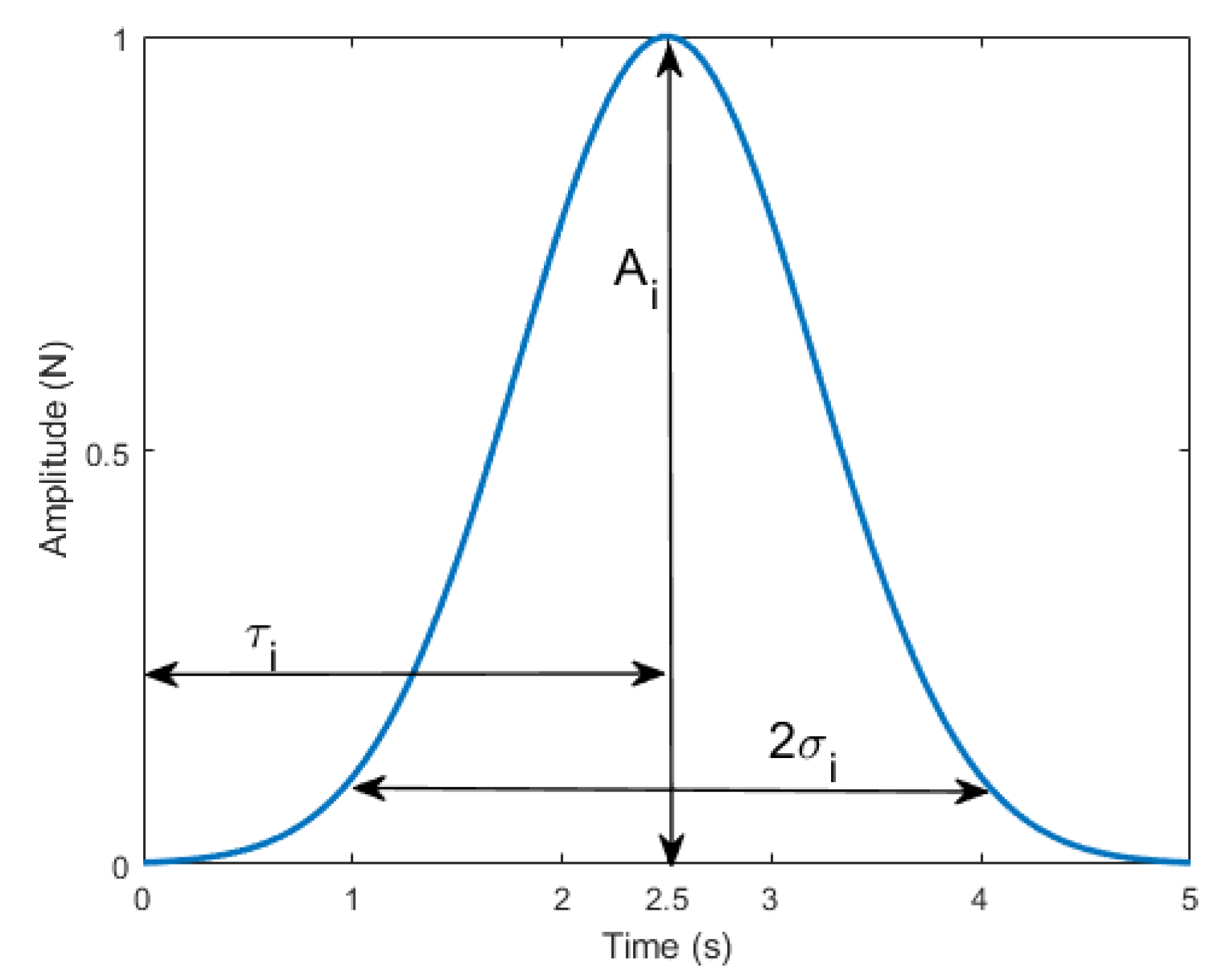
A large part of this research was performed using simulation. Thus, external forces had to be modeled mathematically in a randomized manner, but in such a way that they performed as forces from the real world. A bell-shaped curve was used since it captures the similarity to the real world where the experimenter applied force. Thus, the external force was modeled as:
where , , and are amplitude, time offset, and standard deviation (it defines the width) of the bell-shaped curve, respectively; these definitions are shown in Figure 1. The term is a randomly generated sign (unbiased). n is the number of how many times the external force acts on the robot end-effector in a particular trajectory (the values were integers in the range [5, 15] per measurement instance). Amplitudes, time offsets, and standard deviation were all generated randomly and distributed uniformly (ranges: [5, 20] N, [5, 10] s, and [0.5, 1.5] s, respectively).
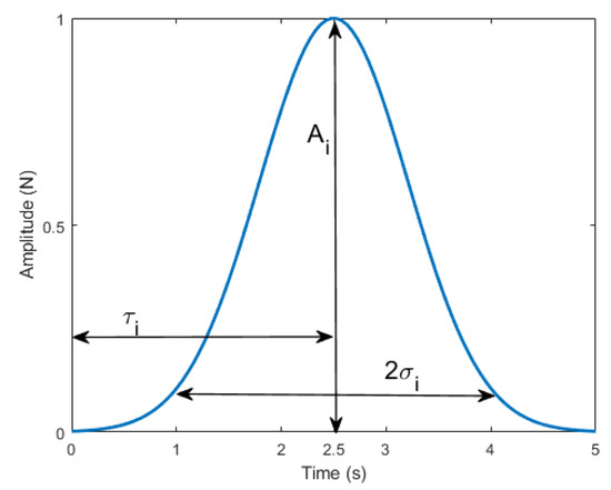
Figure 1.
Bell-shaped curve template used to generate external forces.
There were 1000 measurement instances with between 5 and 50 valid trajectories executed in each. For trajectory generation, first, a valid goal was generated randomly (uniform, in joint space), then a trajectory to that goal from the present robot state was planned using Open Planning Library [24] and its default planning algorithm, the Rapidly-exploring Random Tree (RRT) Connect algorithm. If no trajectory was found, the procedure was repeated until a valid trajectory was found. Between the execution of trajectories, there was a 1 s standstill.
The data set was split in the following manner: The test set was created by randomly selecting 20% of data instances, and the other 80% was used for training and validation purposes. Furthermore, a random 20% (or 16% in terms of total data instances) was used as a validation set, and the rest was used as a training set. As such, the training set consisted of 640 simulation instances, the validation set consisted of 160 simulation instances, and the test set included 200 simulation instances. Note that the same percentage data split was used throughout the manuscript.
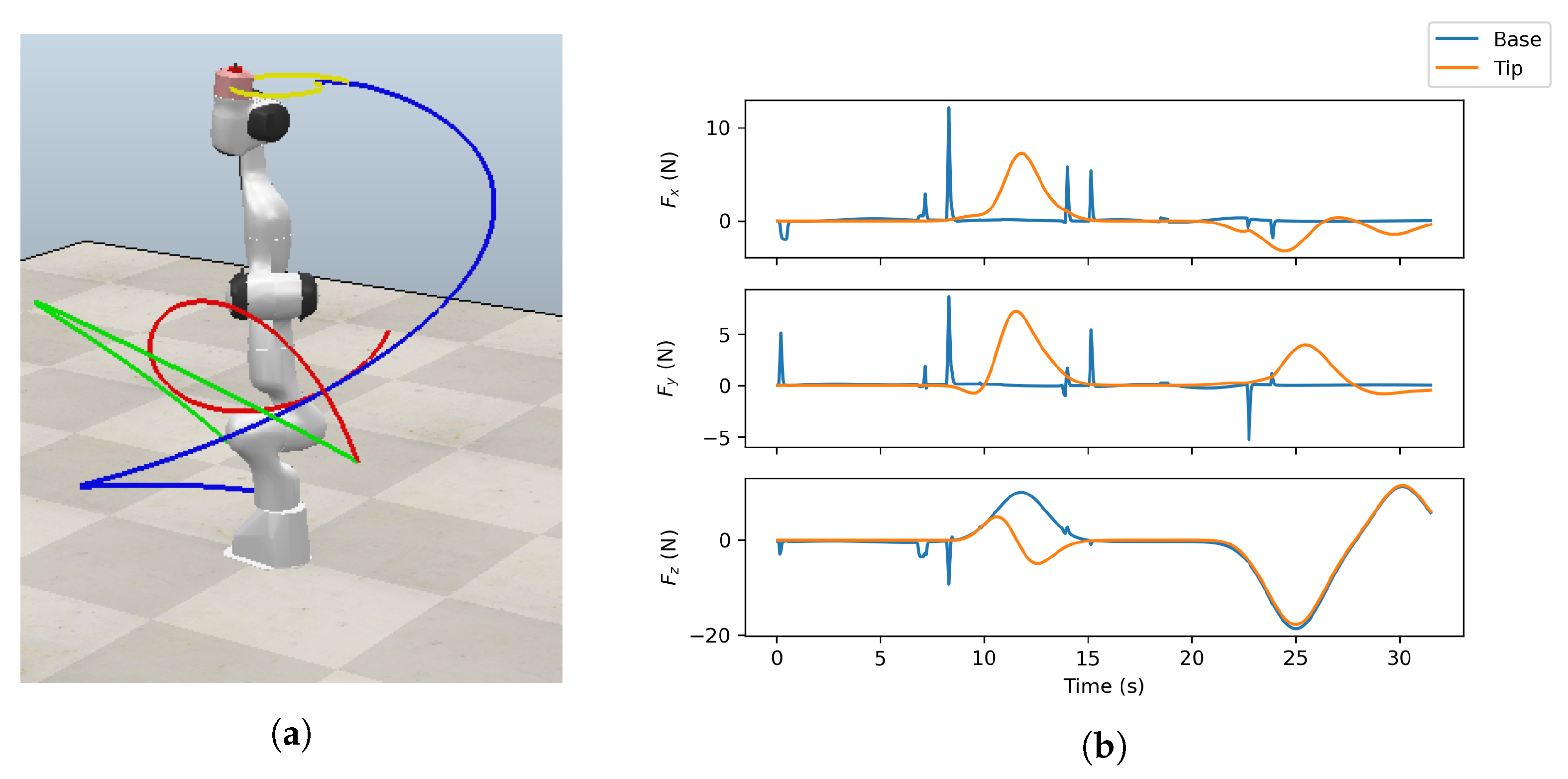
A total of 3,919,800 samples were collected, which took about 48 h in simulation on a computer with an Intel Core i3-6100 processor (Intel Corporation, Santa Clara, CA, USA) with 16 GB RAM, but in practice, it was a shorter time since simulation runs faster than real-time. The simulation engine used for the simulations was provided by the CoppeliaSim environment, and it was the Newton Dynamics engine [25]. The simulation step was set to 50 ms. An example of a simulation ran using the described experimental setup with four visualized trajectories and plotted forces on the base and tip is shown in Figure 2. Please note that periods may exist without an external force acting on the end-effector during the execution of the trajectories. As such, the data set was made more diverse in order to improve generalization.
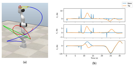
Figure 2.
Example of the simulation run: (a) CoppeliaSim with four visualized trajectories; (b) three corresponding force interactions acting on the base and the end-effector for four visualized trajectories.
Another set of data was collected along with these data, with the same simulation-based setup except that no external forces were acting on the robot end-effector. This approach enabled us to directly compare our (generic) neural network architecture with other approaches from the literature using an elaborate ad hoc neural-network-based architecture such as the one in [19]. It also showcases the possibility of hybrid training: training the network on large amounts of data from simulation (taking into account time and safety considerations) and then using transfer learning based on real-world force interaction measurements.
3.2. Neural Networks
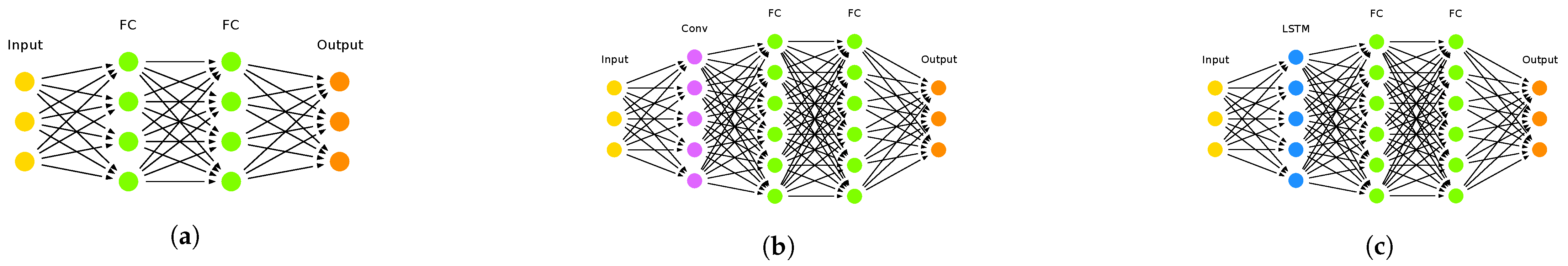
In this study, three different neural network architectures were used: multilayer perceptron (occasionally, the term deep feedforward neural network is used), convolutional neural network, and long short-term memory (LSTM) network. They are conceptually depicted in Figure 3 and are briefly introduced in this subsection. Additionally, a deep Lagrangian network (DeLaN) [19], also introduced in Section 2, was used to compare our presented method for joint torques estimation.
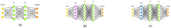
Figure 3.
Conceptual presentations of the network architectures used in this research: (a) multilayer perceptron; (b) 1D-convolutional network; (c) LSTM network.
The multilayer perceptron is the most basic deep learning model and a basis for many other important architectures, including those used in this research. Each neuron in a layer is connected to every neuron in the following layer. Thus, this kind of layer is referred to as a dense layer or fully connected layer.
Convolutional neural networks are a neural network architecture specialized for processing data that “use convolution in place of general matrix multiplication in at least one of their layers” [26]. They are often used to process grid-like data (1D grid for time series data or 2D pixels for images). These networks are an extension of the multilayer perceptron, which assumes that neighboring features are not independent, i.e., they likely belong to the same temporal sequence (in the case of 1D convolution, the one that was used in this research) or the same visual structure (in the case of images). Convolutional neural networks are usually deeper than multilayer perceptrons because they are intended for processing more complex data. Convolutional neural networks begin with a convolution layer whose main characteristic is sparse weights, meaning that, unlike in fully connected layers, every unit is not necessarily connected to all units in the next layer. This connection is achieved because the kernel used in the convolution operation is smaller than the input. A convolutional layer is optionally followed by a pooling layer, which reduces the dimension of the features produced by the convolutional layer. It takes the activated outputs of the convolutional layer producing an output at a location that provides summary statistics about the location’s surroundings. More convolution layers may follow, possibly each followed by a pooling layer. Fully connected layers then follow these layers as in the multilayer perceptron case. Stacking the layers enables convolutional networks to learn based on the features extracted by the convolution(s) rather than learning on raw inputs, which is the case of multilayer perceptrons.
Recurrent neural networks (RNNs) are used to process sequential data, most often temporal sequences. Most notable applications include signal processing and natural language processing. A recurrent neural network contains one or more recurrent layers at the beginning of the network, with fully connected layers following. It is similar to 1D convolutional neural networks in that both have a similar structure, but they are significantly different in how the data are processed in convolutional and recurrent layers. The recurrent layer consists of cells that feature a loop (or feedback), allowing a piece of information to persist between the training steps. In this way, a recurrent neural network may be seen as multiple copies of the same network chained one after another. However, these networks are unable to handle long-term dependencies [27] (finding the connection between previously seen information and the present task). Therefore, long short-term memory (LSTM) networks were introduced [14] to resolve this problem. This architecture was proposed as a replacement to traditional recurrent neural networks and are nowadays used for most applications.
All networks described in this paper were initialized with a Glorot uniform initializer [28], and trained using Adam optimizer [29], starting with a learning rate of 0.001 (the optimizer is adaptive; thus, the learning rate changes during the training). In the training process, the mean squared error (MSE) was used as a loss function, while the Rectified Linear Unit (ReLU) function was used for activating neurons. Finally, as a performance metric, the root mean squared error (RMSE) function was used (only on a test data set). In all instances, the training lasted until there was no improvement in validation loss for five consecutive epochs. The training was conducted using Tensorflow 2.0 and Keras, while the hyperparameter tuning was achieved using the Keras Tuner (hyperparameter tuning library, which is a part of Tensorflow and Keras framework). Note that the loss function (regardless of which set it was calculated on) in architectures that include regularization (as our does) consists of two terms: per-example loss (MSE in our case) and loss due to the regularization (whose impact is defined by user-defined hyperparameters) [26]. The metric only describes the differences between the estimates and the targets (on a per-example basis). This, in turn, implies that the metric in these particular cases is lower or equal to the loss function in its value.
3.3. End-Effector Forces Estimation
Several neural networks of different types of architectures were trained with varying hyperparameters. An overview of the trained neural networks with their respective hyperparameters is summarized in Table 1. Note that these architectures were selected among many other trained architectures by varying different hyperparameters using a trial-and-error approach and our previous experience in the field. However, only the ones presented in Table 1 are discussed here as the best-performing ones among them due to space constraints.

Table 1.
Trained neural networks with selected hyperparameters.
The inputs to the network were the forces measured with the sensor mounted under the robot base, joint positions, velocities and accelerations, and, in some instances, joint torques, as indicated in the table. Joint positions and velocities are usually available from most (if not all) robots and can easily be used in the approach. Although the availability of joint torques (either through direct measurement or estimation from other measured values such as joint motor currents) is becoming more widespread, there is still a number of robot manipulators (mainly educational and more affordable ones) that do not have this feature. The outputs were the forces measured using the sensor mounted on the robot tip. Multilayer perceptron (MLP) networks have a higher number of neurons per layer than other architectures, which is based on our previous experience in the field and the fact that MLP performs the learning on raw input data rather than temporal features (which is the case with convolutional and long short-term memory (LSTM) networks), and thus need more neurons to generalize appropriately. In convolutional and LSTM networks, a single 1D convolution or LSTM layer is used at the beginning of the network, because a single layer is enough to extract interesting temporal features for relatively low-dimensionality and - complexity data. Therefore, the number of units in those layers was fixed to 16 for all training instances.
Following these networks, two more networks were obtained using parameter optimization to obtain more accurate estimates. The optimized hyperparameters were the number of LSTM layers, the number of LSTM units per layer, the number of fully connected layers, the number of units per layer, and the activation function. These networks are included in the table and are marked with *. Contrary to the others, they have two LSTM layers with 32 units each and use ReLU as an activation function. These networks are the best-performing ones selected during the optimization process amongst those considered, with different values of hyperparameters.
The goal of training different architectures of neural networks with different hyperparameters was not to identify the optimal hyperparameters or architecture. Thus, only a small-scale hyperparameter optimization was conducted to assess if there was some improvement in network performance. Instead, the main goal was to identify what architecture is best-suited for the problem at hand and whether the inclusion of additional information provided by the robot as inputs (in our case, joint torques) significantly affects the performance of the neural networks.
3.4. Joint Torques Estimation
Following the training of the neural networks for end-effector force estimation, another experiment was conducted to assess the performance of the robot’s inverse dynamic model approximated by various neural networks and to compare it with the analytical inverse dynamic model identified in [23] and with the DeLaN network [19]. Our inverse dynamic model is also based on neural networks, which take joint positions, velocities, and accelerations and output control torques.
The inverse dynamic model is derived from the Euler–Lagrange equation as
where is the mass matrix, is a term describing centripetal and Coriolis forces, is the gravity term, is the torque due to friction, and is the vector of joint-side torques. All these data are available in the simulation data sets. This experiment differed from the previous in that inputs to the neural network were joint positions, velocities, and accelerations, this time without forces measured by the force/torque sensor, since the inverse dynamics model is not dependent on external forces.
For this experiment, neural networks were trained with simulation data and with real-world data. Thus, additional data were collected on the real-world robot of the same type, in a similar experimental setup as in simulation, where force was applied to the end-effector by the experimenter. There were 260 measurement instances with between 5 and 20 valid trajectories executed in each instance, which resulted in 480 min of pure robot working time. The data sets for neural network training and testing were split in the same ratios as the simulation case. Random trajectories were generated with the same path planning algorithm as in the simulation (RRT-Connect), now within the MoveIt tool [30] implemented as part of the robot operating system (ROS) package MoveIt1. The package is part of the ROS Melodic distribution running on top of Ubuntu 18.04 (Canonical Ltd., London, UK). Control of the Franka robot was possible through the libfranka 0.8.0 package.
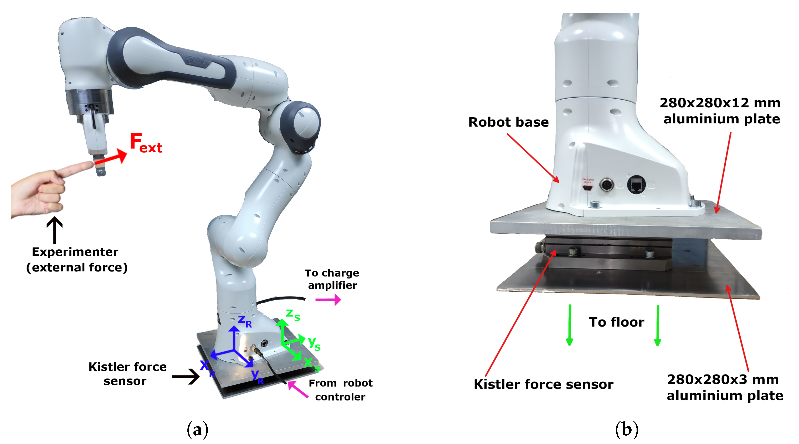
In this experiment, the force sensor was mounted under the robot base between two aluminium plates, as shown in Figure 4. The force sensor used was a Kistler 9257A, with a Kistler 5070A charge amplifier (both by Kistler Instrumente AG, Winterthur, Switzerland) and an NI USB-6009 A/D converter (National Instruments, Austin, TX, USA) for data acquisition. The spatial calibration between the robot’s base and the Kistler 9257A sensor (i.e., two coordinate frames in Figure 4a) was achieved manually using a digital calliper with a resolution of 0.01 mm and accuracy up to 0.03 mm depending on the measuring range.
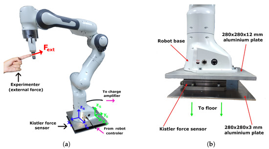
Figure 4.
Real-world experimental setup: (a) Franka robot during measurements with installed sensor under the base; (b) interconnection between the robot base, force sensor, and the environment.
Special consideration was given to the interconnection between the robot base, the Kistler force sensor underneath it, and the environment to ensure the stability and repeatability of robot motion. This is closely depicted in Figure 4b. The robot base was attached at four points defined by the manufacturer via bolts to a rigid aluminium sheet of 280 × 280 × 12 mm. This was then secured to the sensor’s top surface at predefined attachment points with sink-in head screws so that the robot laid flat on the aluminium plate. This was then attached to a 280 × 280 × 12 mm aluminium sheet to provide extra stability when attaching it to the environment (e.g., floor). special care was given to robot pose positioning relative to the sensor surface underneath to place a base footprint as large as possible robot over it and ensure that, in the initial configuration, the whole system was balanced (i.e., even without the bolts and screws).
4. Results and Discussion
4.1. End-Effector Force Estimation—Simulation Experiment
The results for the neural networks trained using the data obtained on the Franka robot in the simulation are shown in Table 2 with row numbers corresponding to the architectures in Table 1.
Table 2.
Network losses and RMSE for Franka robot during simulation.
From these results, it is apparent that the performance of the Franka robot significantly improved, i.e., that force estimates were much more accurate than those presented in our previous research [31]. When interpreting the values presented in the table, it should be kept in mind (as outlined in Section 3) that the loss function contains a regularization term which is the result of a training/learning procedure. This value might differ for each of the eleven individual cases (rows) in the table since they are separate learning instances. Thus, it is impossible to directly compare loss function trends and metric values. However, comparison within a loss function or metric is possible. This holds for all other instances within the manuscript with the same parameters.
The Franka robot state has many other features in addition to joint positions: joint velocities, accelerations, and torques. Consequently, there are more features to learn on; thus, the inverse dynamics of the Franka robot can be better captured using these features. Moreover, since joint velocities and accelerations are the inputs of any inverse dynamics model, it makes the accurate learning of inverse dynamics possible. However, inverse dynamics is learned implicitly using this approach as part of an end-to-end neural network for end-effector force estimation.
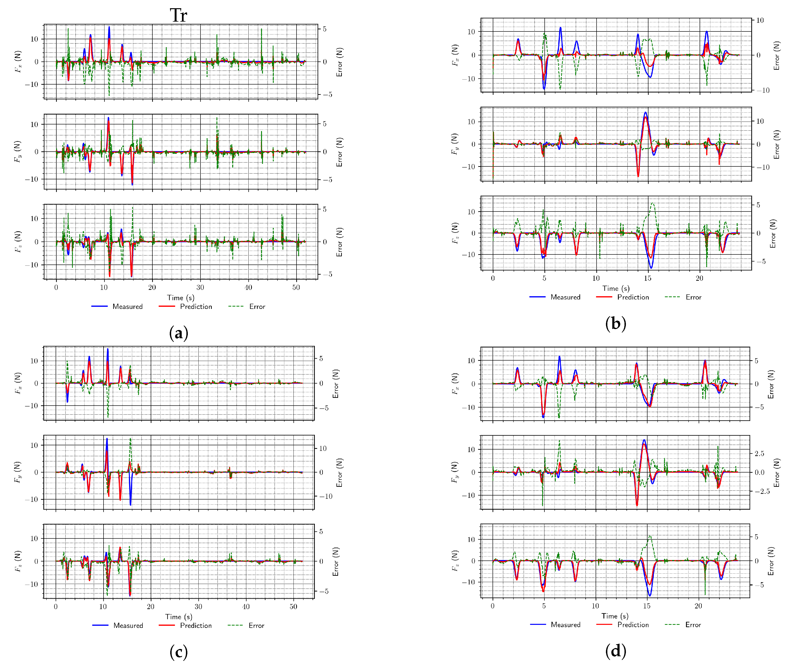
It is also noticeable from the results that networks operating on sequential inputs perform better than MLP networks. However, also among those, LSTM networks provide significantly better performance than convolutional ones. Moreover, when using longer sequences of input data (five samples vs. ten samples), the performance was improved. Finally, the inclusion of additional data about the robot state (joint torques) is also beneficial (as per the RMSE), since it improved the performance for each of the trained architectures compared with the performance of networks of the same architectures when those data were not used for about 15%. We think that the RMSE is more relevant when analyzing network performance since the produced RMSE value includes only the error between targets and estimates, while loss, along with those, includes a component due to regularization loss. A similar trend is noticeable in the optimized network architectures. Example force predictions from the test set using the trained networks are shown in Figure 5 (the architectures correspond to those defined in Table 1).
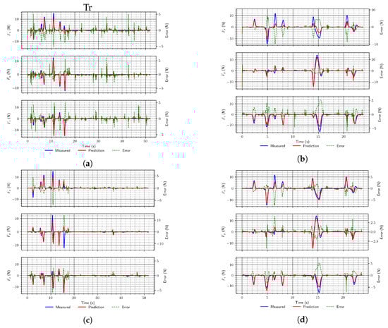
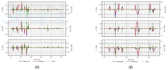
Figure 5.
Two random examples (a,c,e and b,d, and f, respectively) of end-effector force predictions using the simulation data test set for different types of proposed network architectures. (a) MLP (arch. #2); (b) MLP (arch. #3); (c) Convolutional (arch. #4); (d) Convolutional (arch. #6); (e) LSTM (arch. #7); (f) LSTM (arch. #9).
This good performance might have been obtained in part because the data for training these networks were collected in simulation, and the simulation is only an approximation of the real world (i.e., less complex than the real world), so it is expected that the approach would perform better in simulation than in the real world.
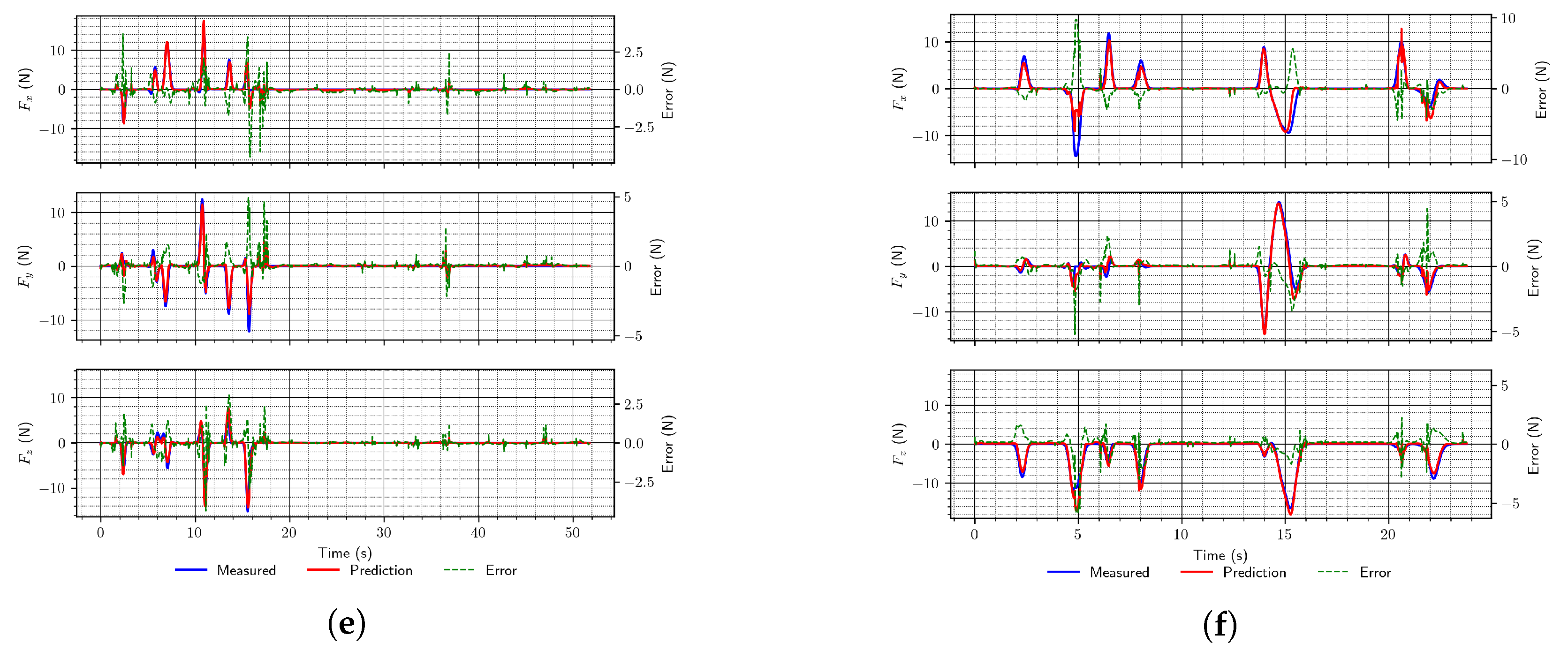
The hyperparameter optimization that was performed yielded networks that produced somewhat better estimates, which is shown in Figure 6. The optimized network that used a data set with joint torques performed better than one without it, according to the RMSE (0.1533 vs. 0.1647). Additionally, from the figure, it can be seen that estimates are better for all three axes, and errors are smaller than with the presented networks that were not optimized.
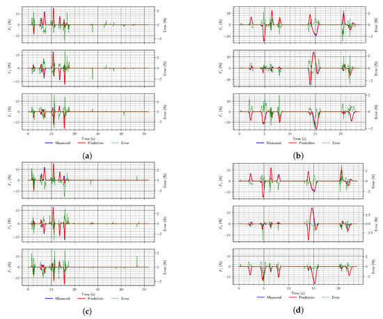
Figure 6.
Examples of end-effector force predictions using the simulation data test set for optimized LSTM architectures. (a) Optimized LSTM (arch. #10); (b) optimized LSTM (arch. #10); (c) optimized LSTM (arch. #11); (d) optimized LSTM (arch. #11).
4.2. Joint Torques Estimation—Simulation and Real-World Experiment
In this subsection, all obtained results regarding joint torque estimation are reported and summarized in Table 3. The results obtained for the same experiment using simulation data sets are reported first, followed by the results obtained using real-world data sets.
Table 3.
Joint torque estimation summary.
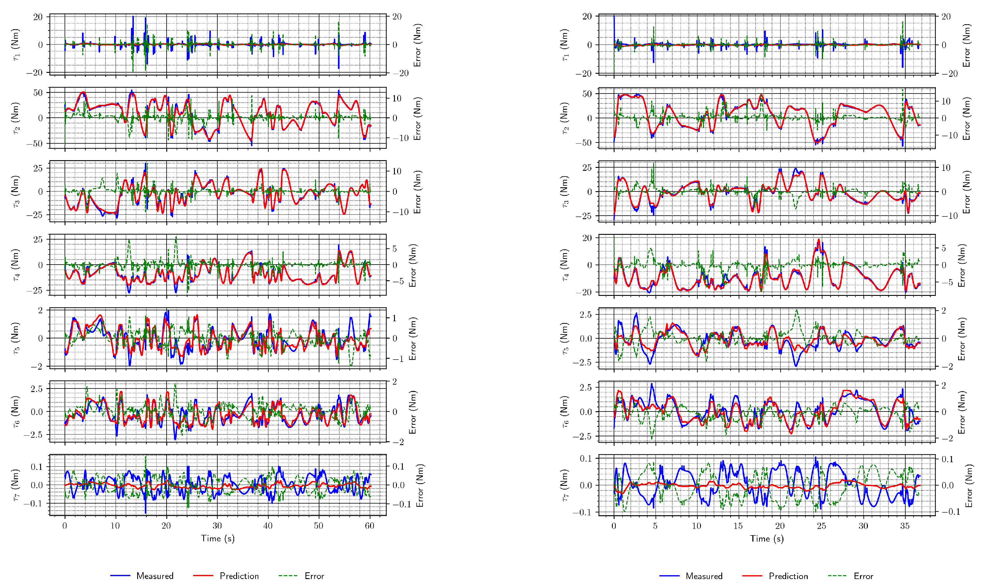
The torques were first estimated using the DeLaN architecture, proposed in [19]. In that paper, the experiment that was conducted considered only four lower joints, since they “dominate dynamics” [19]. In our research, we trained the DeLaN network for all seven joints with the data set that had no external forces acting and obtained reasonably good estimates, as shown in the two examples in Figure 7.
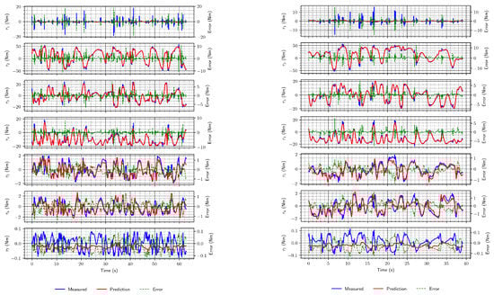
Figure 7.
Two examples of torque estimates using the DeLaN architecture without external forces acting.
From Figure 7, it is evident that the primary sources of inconsistency between the actual and estimated torque plots/trajectories are joints 1 and 7. However, their relative contribution to the total error differs since they pertain to different torque scales as depicted by the y axis ranges in the figure.
Predictions for joint 1 are inaccurate due to the peaks in the torque in the moments the robot starts or stops moving, which could not be learned easily by this architecture. In addition to the peaks that are rare during the whole measurement sequence, joint torques for this joint have small values, and thus it seems as if the network is filtering out the peaks. On the other hand, with joint 7, estimates are inconsistent, but this may not be a critical issue since this joint contributes least to the whole robot dynamics. Additionally, similar to joint 1, the torque values are minimal compared to the torques for other joints (i.e., other joint torques are at least one order of magnitude higher, often more).
When this architecture was trained on the data set with external forces acting, the results were slightly worse: the validation and test data sets resulted in higher losses, and the estimates were not overlapping for the most part. This is also in line with the significantly worsened RMSE, which does not contain a regularization term as do loss functions. The examples are shown in Figure 8. The performance of this network is generally similar to the previous case, with observations about joints 1 and 7 holding. However, the estimates are somewhat less accurate for other joints than in the previous case. When trained using a data set with external forces, this network appears to neglect external forces, i.e., the predictions are as if there is no external force acting, which is especially visible in the estimates of joints 5 and 6, and on joint 4, to a lesser extent.
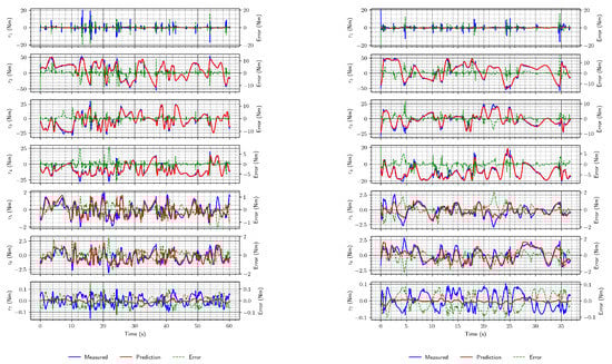
Figure 8.
Two examples of torque estimates using the DeLaN architecture with external forces acting.
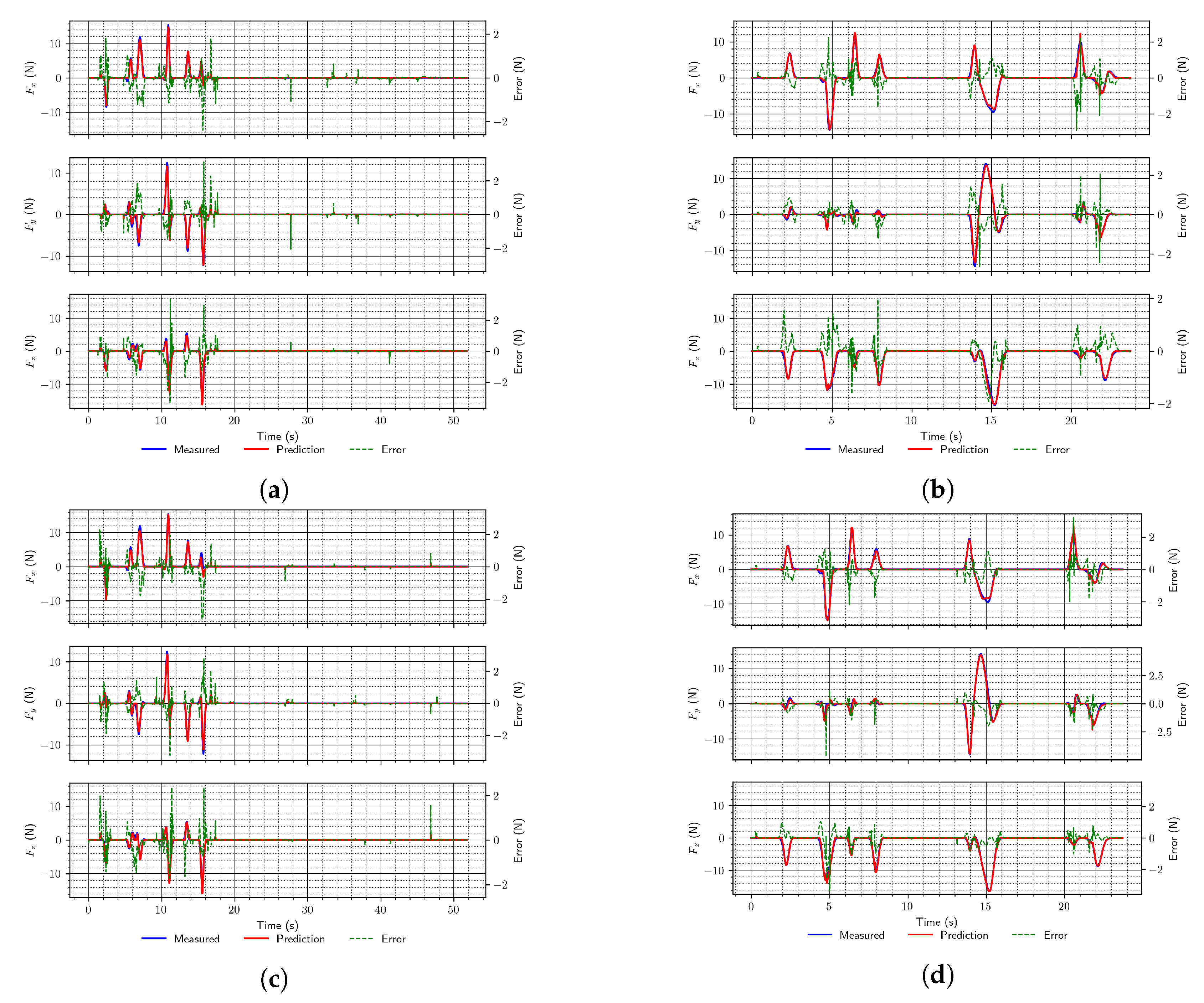
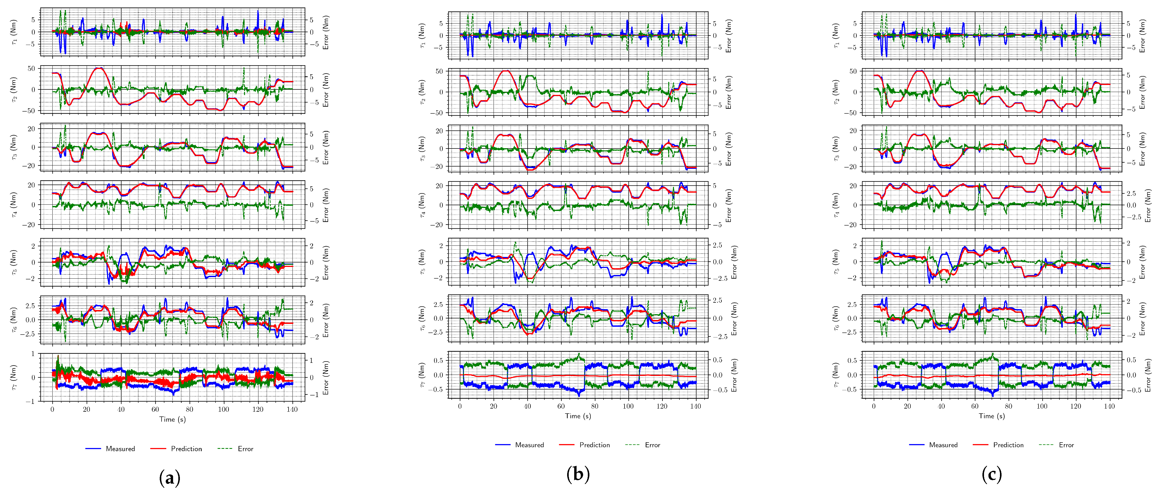
Classical neural network architectures, especially LSTMs (which operate on sequences), perform well when external forces act on the robot, as shown in Figure 9. Their estimates are even better than the DeLaN estimates (supported by RMSE values obtained on the test set, in Table 3), which leads to the conclusion that this architecture is well-suited for the task.
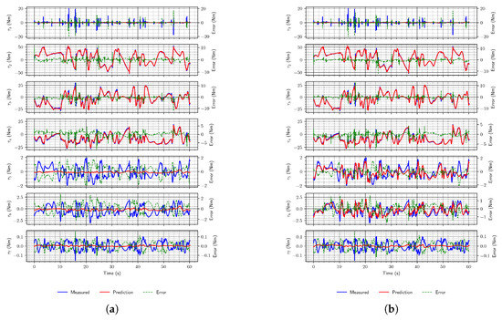
Figure 9.
Example torque estimates using convolutional and LSTM network. (a) Convolutional network; (b) LSTM network.
Finally, the DeLaN network performs better when no external forces are acting, a case that is not particularly useful for real applications but shows that this architecture captures the robot’s dynamic model best (among those tested).
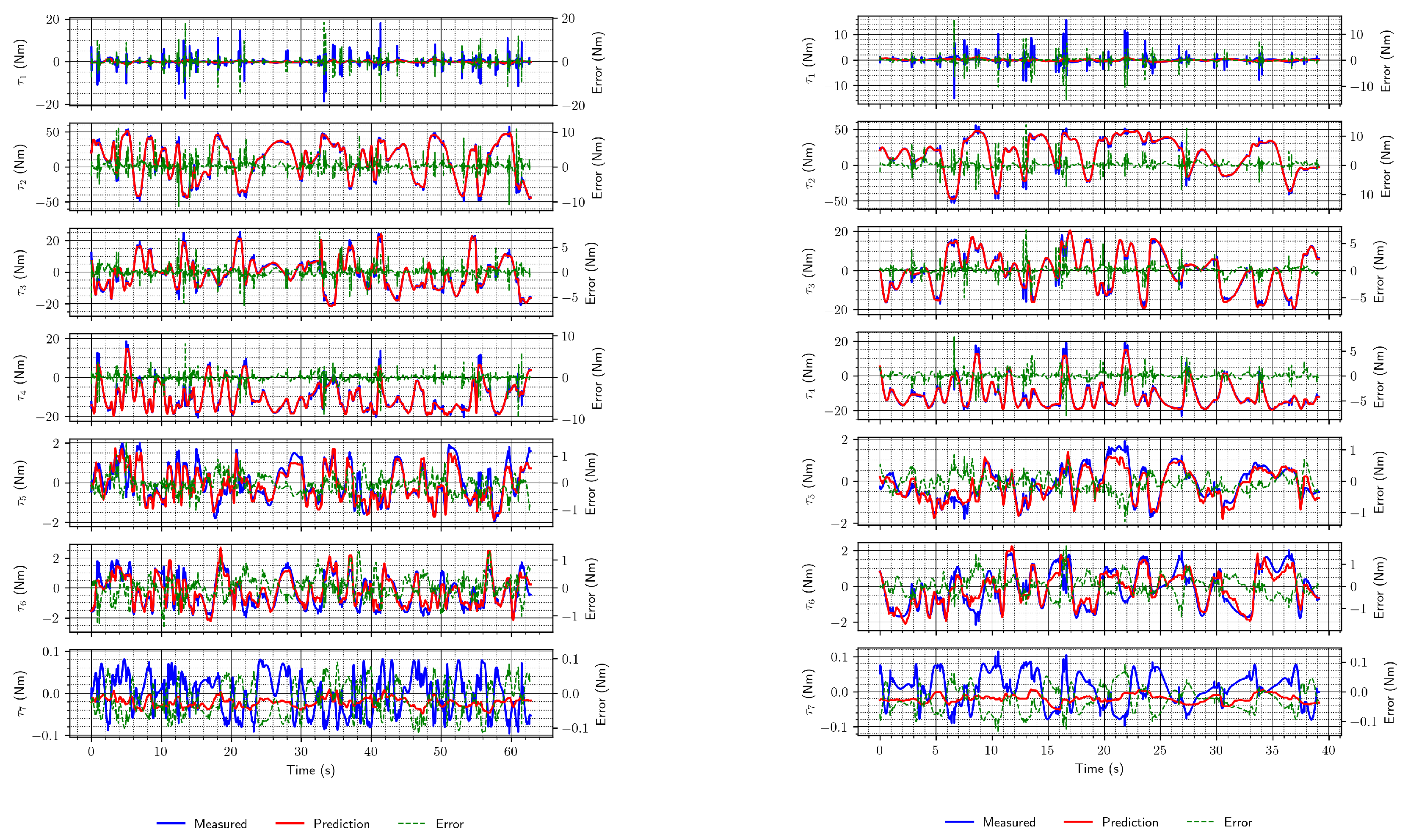
The results obtained using data from the simulation were then compared to the ones from the real world. They are numerically (RMSE) and visually (Figure 10) slightly worse than those from the simulation, but the same trends are followed. Thus, again, the LSTM network was identified as the one that performs the best.
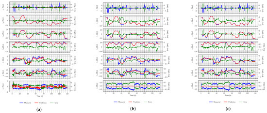
Figure 10.
Example torque estimates on the real-world data sets. (a) DeLaN; (b) convolutional network; (c) LSTM network.
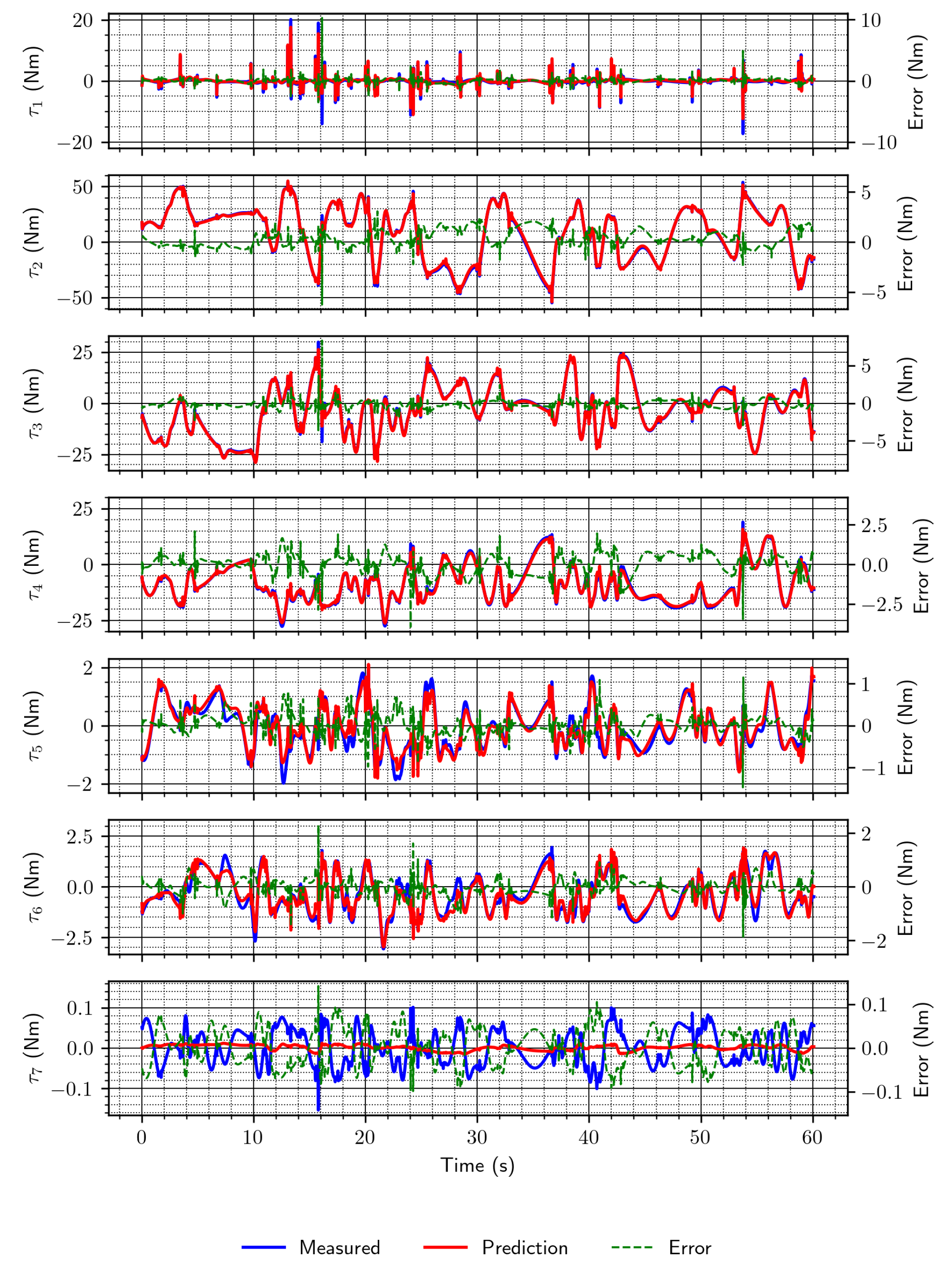
In the case of joint torques estimation, hyperparameter optimization was also performed. Again, a network with two LSTM layers with 32 units each was identified as best (among those considered during the optimization process). However, this time, the two fully connected layers had only eight units each, and the activation function was different; this time, hyperbolic tangent was chosen instead of ReLU (in Table 3, this architecture is marked with an asterisk). This network performed better than those that were not optimized. This is especially evident in Figure 11, where improvements in the estimates for joints 1, 5, and 6 can be seen. Joint 1 peak predictions are now mostly correct, and joints 5 and 6 mostly follow the measured values, thus reducing the error. The optimization was also performed using a real-world data set. The obtained architecture was identical to that obtained using the simulation data set, but since the RMSE value was worse, this network was not considered further.
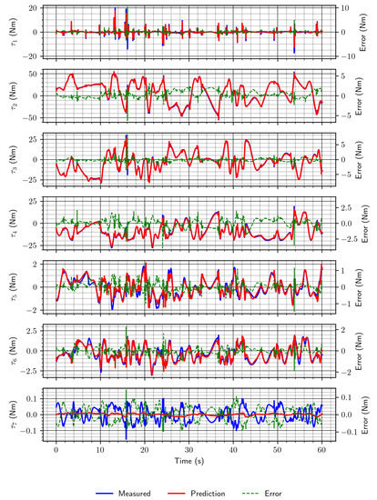
Figure 11.
Example joint torque estimates for optimized LSTM network.
If the proposed approach is to be applied in real-world settings, especially for human–robot (force-based) interactions, the safety of the approach needs to be discussed (but this was not the focus of this research). Assuming that the network was trained appropriately (with a sufficient amount and variety of data), additional potential sources of network malfunction (in terms of safety) could be faulty sensor readings and adversarial attacks on the network. Faulty sensor issues could be addressed by one of the fault diagnosis algorithms [32] (which include neural networks) before the data are fed to our network. This is an issue in all force measurement and estimation approaches regardless of which algorithm is used. Adversarial attacks on convolutional networks are well-documented and known [33], but these types of attacks are becoming more and more present in recurrent-type networks, including LSTM. Fortunately, countermeasures exist [34] and can be deployed in real-world scenarios.
5. Conclusions
This paper presented the methods for robot end-effector force estimation and joint torque estimation. Both methods are based on deep neural networks, and contrary to traditionally used methods, knowledge about robot dynamics is not required since it is learned implicitly during the training of the network. The methods were first trained with the data obtained in simulation, which enabled collecting an abundance of data with minimal risk and controlling all of the parameters. The results for both methods identified the LSTM network as the best architecture among those considered. The approach to joint torque estimation was then tested on data obtained on a real-world robot. The obtained results are slightly worse than those from the simulation, but generally, the estimates behave very similarly, demonstrating the approach’s validity. Since the research goal was to assess the validity of the proposed approach, only a small-scale optimization was performed, which identified better-performing network architectures. Thus, large-scale optimization could be performed in future research on the topic, possibly leading to even better performance.
We plan to extend our research to include end-effector force estimates for the real Franka robot and try the approach on other models, both in simulation and the real world. Furthermore, we plan to extend the approach so that a neural network is used to correct the error in the predictions produced by the analytical/identified model, possibly by incorporating the analytical model into the loss function and integrating the approach on a real-world mobile manipulator. Finally, we plan to explore the use of an array of simple 1D strain gauges under the robot base (in place of more expensive force/torque sensors) to estimate robot joint torques and interaction forces, which would be more applicable to educational robots where budgeting is of importance.
Author Contributions
Conceptualization, S.K. and J.M.; formal analysis, S.K., J.M. and R.K.; methodology, S.K., J.M. and R.K.; software, S.K.; supervision, V.P.; validation, J.M.; visualization, S.K.; writing—original draft, S.K.; writing—review and editing, J.M., R.K. and V.P. All authors have read and agreed to the published version of the manuscript.
Funding
This research received no external funding.
Acknowledgments
Authors would like to express gratitude to Marko Mladineo and Sonja Jozić from Faculty of Electrical Engineering, Mechanical Engineering and Naval Architecture, University of Split, for making their hardware available for use for the real-world experiment.
Conflicts of Interest
The authors declare no conflict of interest.
Abbreviations
The following abbreviations are used in this manuscript:
| GPU | Graphics Processing Unit |
| MLP | Multilayer perceptron |
| LSTM | Long Short-term Memory |
| DeLaN | Deep Lagrangian Network |
| LNN | Lagrangian Neural Network |
| RNN | Recurrent Neural Network |
| ReLU | Rectified Linear Unit |
| MSE | Mean squared error |
| RMSE | Root-mean-square error |
| ROS | Robot Operating System |
References
- Siciliano, B.; Villani, L. Robot Force Control; Springer: Berlin/Heidelberg, Germany, 1999. [Google Scholar] [CrossRef]
- Song, A.; Fu, L.F. Multi-dimensional force sensor for haptic interaction: A review. Virtual Real. Intell. Hardw. 2019, 1, 121–135. [Google Scholar] [CrossRef] [Green Version]
- Sebastian, G.; Li, Z.; Crocher, V.; Kremers, D.; Tan, Y.; Oetomo, D. Interaction Force Estimation Using Extended State Observers: An Application to Impedance-Based Assistive and Rehabilitation Robotics. IEEE Robot. Autom. Lett. 2019, 4, 1156–1161. [Google Scholar] [CrossRef]
- Alcocer, A.; Robertsson, A.; Valera, A.; Johansson, R. Force estimation and control in robot manipulators. IFAC Proc. Vol. 2003, 36, 55–60. [Google Scholar] [CrossRef]
- Hacksel, P.; Salcudean, S. Estimation of environment forces and rigid-body velocities using observers. In Proceedings of the 1994 IEEE International Conference on Robotics and Automation, San Diego, CA, USA, 8–13 May 1994. [Google Scholar] [CrossRef]
- Ohishi, K.; Miyazaki, M.; Fujita, M.; Ogino, Y. H∞ observer based force control without force sensor. In Proceedings of the IECON ’91: 1991 International Conference on Industrial Electronics, Control and Instrumentation, Kobe, Japan, 28 October–1 November 1991. [Google Scholar] [CrossRef]
- Eom, K.; Suh, I.; Chung, W.; Oh, S.R. Disturbance observer based force control of robot manipulator without force sensor. In Proceedings of the 1998 IEEE International Conference on Robotics and Automation (Cat. No.98CH36146), Leuven, Belgium, 20–20 May 1998. [Google Scholar] [CrossRef]
- Stolt, A.; Linderoth, M.; Robertsson, A.; Johansson, R. Force controlled robotic assembly without a force sensor. In Proceedings of the 2012 IEEE International Conference on Robotics and Automation, Saint Paul, MN, USA, 14–18 May 2012. [Google Scholar] [CrossRef] [Green Version]
- Liu, S.; Wang, L.; Wang, X.V. Sensorless force estimation for industrial robots using disturbance observer and neural learning of friction approximation. Robot. Comput.-Integr. Manuf. 2021, 71, 102168. [Google Scholar] [CrossRef]
- el Dine, K.M.; Sanchez, J.; Corrales, J.A.; Mezouar, Y.; Fauroux, J.C. Force-Torque Sensor Disturbance Observer Using Deep Learning. In Springer Proceedings in Advanced Robotics; Springer International Publishing: Cham, Switzerland, 2020; pp. 364–374. [Google Scholar] [CrossRef] [Green Version]
- van Damme, M.; Beyl, P.; Vanderborght, B.; Grosu, V.; van Ham, R.; Matthys, A.; Lefeber, D. Estimating robot end-effector force from noisy actuator torque measurements. In Proceedings of the 2011 IEEE International Conference on Robotics and Automation, Shanghai, China, 9–13 May 2011. [Google Scholar] [CrossRef]
- Wahrburg, A.; Bos, J.; Listmann, K.D.; Dai, F.; Matthias, B.; Ding, H. Motor-Current-Based Estimation of Cartesian Contact Forces and Torques for Robotic Manipulators and Its Application to Force Control. IEEE Trans. Autom. Sci. Eng. 2018, 15, 879–886. [Google Scholar] [CrossRef]
- Levine, S.; Pastor, P.; Krizhevsky, A.; Ibarz, J.; Quillen, D. Learning hand-eye coordination for robotic grasping with deep learning and large-scale data collection. Int. J. Robot. Res. 2017, 37, 421–436. [Google Scholar] [CrossRef]
- Jin, L.; Li, S.; Yu, J.; He, J. Robot manipulator control using neural networks: A survey. Neurocomputing 2018, 285, 23–34. [Google Scholar] [CrossRef]
- Bousmalis, K.; Irpan, A.; Wohlhart, P.; Bai, Y.; Kelcey, M.; Kalakrishnan, M.; Downs, L.; Ibarz, J.; Pastor, P.; Konolige, K.; et al. Using Simulation and Domain Adaptation to Improve Efficiency of Deep Robotic Grasping. In Proceedings of the 2018 IEEE International Conference on Robotics and Automation (ICRA), Brisbane, Australia, 21–26 May 2018. [Google Scholar] [CrossRef] [Green Version]
- Smith, A.C.; Hashtrudi-Zaad, K. Application of neural networks in inverse dynamics based contact force estimation. In Proceedings of the 2005 IEEE Conference on Control Applications (CCA 2005), Toronto, ON, Canada, 28–31 August 2005. [Google Scholar] [CrossRef]
- Marban, A.; Srinivasan, V.; Samek, W.; Fernández, J.; Casals, A. A recurrent convolutional neural network approach for sensorless force estimation in robotic surgery. Biomed. Signal Process. Control 2019, 50, 134–150. [Google Scholar] [CrossRef] [Green Version]
- Aviles, A.I.; Alsaleh, S.; Sobrevilla, P.; Casals, A. Sensorless force estimation using a neuro-vision-based approach for robotic-assisted surgery. In Proceedings of the 2015 7th International IEEE/EMBS Conference on Neural Engineering (NER), Montpellier, France, 22–24 April 2015. [Google Scholar] [CrossRef] [Green Version]
- Lutter, M.; Ritter, C.; Peters, J. Deep Lagrangian Networks: Using Physics as Model Prior for Deep Learning. In Proceedings of the International Conference on Learning Representations, New Orleans, LA, USA, 6–9 May 2019. [Google Scholar]
- Cranmer, M.; Greydanus, S.; Hoyer, S.; Battaglia, P.; Spergel, D.; Ho, S. Lagrangian Neural Networks. In Proceedings of the ICLR 2020 Workshop on Integration of Deep Neural Models and Differential Equations, Addis Ababa, Ethiopia, 26 April 2020. [Google Scholar]
- Greydanus, S.; Dzamba, M.; Yosinski, J. Hamiltonian Neural Networks. arXiv 2019, arXiv:1906.01563. [Google Scholar]
- Rohmer, E.; Singh, S.P.N.; Freese, M. CoppeliaSim (formerly V-REP): A Versatile and Scalable Robot Simulation Framework. In Proceedings of the International Conference on Intelligent Robots and Systems (IROS), Tokyo, Japan, 3–7 November 2013. [Google Scholar]
- Gaz, C.; Cognetti, M.; Oliva, A.; Giordano, P.R.; Luca, A.D. Dynamic Identification of the Franka Emika Panda Robot with Retrieval of Feasible Parameters Using Penalty-Based Optimization. IEEE Robot. Autom. Lett. 2019, 4, 4147–4154. [Google Scholar] [CrossRef] [Green Version]
- Sucan, I.A.; Moll, M.; Kavraki, L.E. The Open Motion Planning Library. IEEE Robot. Autom. Mag. 2012, 19, 72–82. [Google Scholar] [CrossRef] [Green Version]
- Massera, G.; Cangelosi, A.; Nolfi, S. Evolution of Prehension Ability in an Anthropomorphic Neurorobotic Arm. Front. Neurorobotics 2007, 1, 4. [Google Scholar] [CrossRef] [PubMed] [Green Version]
- Goodfellow, I.; Bengio, Y.; Courville, A. Deep Learning; MIT Press: Cambridge, MA, USA, 2016. [Google Scholar]
- Bengio, Y.; Simard, P.; Frasconi, P. Learning long-term dependencies with gradient descent is difficult. IEEE Trans. Neural Netw. 1994, 5, 157–166. [Google Scholar] [CrossRef] [PubMed]
- Glorot, X.; Bengio, Y. Understanding the difficulty of training deep feedforward neural networks. In Proceedings of the Machine Learning Research, Proceedings of the Thirteenth International Conference on Artificial Intelligence and Statistics, PMLR, Chia Laguna Resort, Sardinia, Italy, 13–15 May 2010; Teh, Y.W., Titterington, M., Eds.; MIT Press: Cambridge, MA, USA, 2010; Volume 9, pp. 249–256. [Google Scholar]
- Kingma, D.P.; Ba, J. Adam: A Method for Stochastic Optimization. arXiv 2014, arXiv:1412.6980. [Google Scholar]
- Coleman, D.; Sucan, I.; Chitta, S.; Correll, N. Reducing the Barrier to Entry of Complex Robotic Software: A MoveIt! Case Study. J. Softw. Eng. Robot. 2014, 5, 3–16. [Google Scholar] [CrossRef]
- Kružić, S.; Musić, J.; Kamnik, R.; Papić, V. Estimating Robot Manipulator End-effector Forces using Deep Learning. In Proceedings of the 2020 43rd International Convention on Information, Communication and Electronic Technology (MIPRO), Opatija, Croatia, 28 September–2 October 2020. [Google Scholar] [CrossRef]
- Li, D.; Wang, Y.; Wang, J.; Wang, C.; Duan, Y. Recent advances in sensor fault diagnosis: A review. Sens. Actuators Phys. 2020, 309, 111990. [Google Scholar] [CrossRef]
- Heaven, D. Why deep-learning AIs are so easy to fool. Nature 2019, 574, 163–166. [Google Scholar] [CrossRef] [PubMed]
- Rosenberg, I.; Shabtai, A.; Elovici, Y.; Rokach, L. Defense Methods Against Adversarial Examples for Recurrent Neural Networks. arXiv 2019, arXiv:1901.09963. [Google Scholar]

Publisher’s Note: MDPI stays neutral with regard to jurisdictional claims in published maps and institutional affiliations. |
© 2021 by the authors. Licensee MDPI, Basel, Switzerland. This article is an open access article distributed under the terms and conditions of the Creative Commons Attribution (CC BY) license (https://creativecommons.org/licenses/by/4.0/).