Cryptocurrencies and Tokens Lifetime Analysis from 2009 to 2021

Abstract

The success of Bitcoin has spurred emergence of countless alternative coins with some of them shutting down only few weeks after their inception, thus disappearing with millions of dollars collected from enthusiast investors through initial coin offering (ICO) process. This has led investors from the general population to the institutional ones, to become skeptical in venturing in the cryptocurrency market, adding to its highly volatile characteristic. It is then of vital interest to investigate the life span of available coins and tokens, and to evaluate their level of survivability. This will make investors more knowledgeable and hence build their confidence in hazarding in the cryptocurrency market. Survival analysis approach is well suited to provide the needed information. In this study, we discuss the survival outcomes of coins and tokens from the first release of a cryptocurrency in 2009. Non-parametric methods of time-to-event analysis namely Aalen Additive Hazards Model (AAHM) trough counting and martingale processes, Cox Proportional Hazard Model (CPHM) are based on six covariates of interest. Proportional hazards assumption (PHA) is checked by assessing the Kaplan-Meier estimates of survival functions at the levels of each covariate. The results in different regression models display significant and non-significant covariates, relative risks and standard errors. Among the results, it was found that cryptocurrencies under standalone blockchain were at a relatively higher risk of collapsing. It was also found that the 2013–2017 cryptocurrencies release was at a high risk as compared to 2009–2013 release and that cryptocurrencies for which headquarters are known had the relatively better survival outcomes. This provides clear indicators to watch out for while selecting the coins or tokens in which to invest.

1. Introduction

Cryptocurrencies are digital currencies in which transactions are verified and records maintained by decentralized systems known as blockchains. Blockchains use cryptography or a third-free peer-to-peer electronic system, rather than a centralized trade in which transactions are made by the banks (Angela 2016). Transacting a cryptocurrency is mobile, non-taxable and does not require bank intermediary. Blundell-Wignall (2014) points that digital cash cannot have multiple copies. Hence, a cryptocurrency cannot be used more than once, unlike the bank services where multiple transfers are common.

Cryptocurrecies operate either as coins or tokens. Crypto-coins are native from their own blockchain whilst tokens are built on top of another existing blockchain (Wu et al. 2018). An important number of cryptocurrencies use Euthereum network as an alternative to standalone. Many other known networks include Waves, Stellar, Nem, Couterparty, Bitshares, Achain, Omni, Neo, Ardor, Qtum, Icon and Ubiq. The discretion in cryptocurrency transaction makes a more secure and reliable modern mode of payment as suggest manuscripts such as Blundell-Wignall (2014); Hendrickson et al. (2016) or Urquhart (2016).

The cryptocurrencies release started with the Bitcoin in 2009 Blundell-Wignall (2014). The other popular cryptocurrencies that followed include Litecoin (2011), Peercoin (2012), Ripple (2012), Alphacoin (2013–2014) and Aircoin (2014–2016). As for the year 2021, the new cryptocurrencies include Bogged Finance (2021) and Recharge Finance (2020). The total number of cryptocurrencies in 2021 exceeds 6000 in which around 2000 are inactive (or dead) (Best 2022). The high rate of death of cryptocurrencies has been a barrier of many investors. The risk of collapsing of a number of cryptocurrencies has persuaded some governments to ban such digital financial markets with argument that cryptocurrency trade could facilitate illegal transactions and disrupting the government activities (Hendrickson et al. 2016). However, El Salvador officially adopted Bitcoin as legal tender on 9 June 2021, making it the first country to do so (Thul 2021). In some other countries such as Panama, Brasil, Paraguay, Mexico and Argentina, the governments are hand in hand with the researchers on sustainability of Bitcoin for a future adoption (Thul 2021).

In 2020, the globe was under a relatively rising situation of the outbreak of COVID-19 and at the same time, the relatively high degree spillover of Bitcoin was observed (Xiao et al. 2021). The trade of cryptocurrencies was then globally affected (Youssef et al. 2021). Azimli (2020) suggests that COVID-19 pandemic impacts the financial market through the high level of economic policy uncertainty. The unknown future situation of COVID-19 leads to low cash flow expectations, resulting in possible stock market depreciation (Azimli 2020).

Several studies on cryptocurrencies emerged in many domains such as Mathematical Sciences, Financial Economics and Engineering. Mathematical and statistical modeling on cryptocurrency is found for example in (Gatabazi et al. 2019a, 2019b, 2019c, 2019d) and Chan et al. (2017). Mba and Wang (2019) used copula in describing cryptocurrencies in financial economics framework, a field in which many other manuscripts including Urquhart (2016) and Angela (2016) analyse cryptocurrencies. However, the scientific analysis on the lifetime of cryptocurrencies is not yet popular. To understand the event history analysis of cryptocurrencies and the associated factors may adopt another insight by which the researcher may predict accurately the future of these digital currencies.

The present study uses the time-to-event data analysis for estimating the life-time and the factors of death for cryptocurrencies during the study time ranging from 2009 to 2021.

In addition to the introductory section, the study is subdivided as follows: Section 2 presents the methodology of the study. Section 3 presents the main results and interpretation and Section 4 gives a conclusion.

2. Methodology

This part introduces the time-to-event analysis, discusses the time-to-event regression analysis and then presents the dataset of interest. Preliminary analysis will be displayed by the graphs and the useful statistical tests.

2.1. Concept of the Time-to-Event Data Analysis

The time-to-event analysis or survival analysis aims at making the inference of the time elapsed between the onset of observations until the occurrence of some event of interest. The related regression model expresses the dependence of time-to-event on predictor variables. Methods used in general statistical analysis, in particular in regression analysis, are not directly applicable to survival data due to censoring and truncation. Hosmer et al. (2008) describe three types of censoring: right censoring arising when an individual is not subject to the event until the end of study due to either loss to follow up, or the event has not occurred at the end of the study, or the event has occurred from another cause not related to the cause of interest. Left censoring arises when an individual experienced an event before the onset of the study. Interval censoring refers to when the event occurs within some interval in the study time, or the individual dropped out or observed the event at an unknown time before study termination for reasons unrelated to the study, or the individual was lost to follow-up in an interval between two specified time points. Two types of truncation described in Klein and Moeschberger (2003) are the left truncation and the right truncation. Left truncation occurs when subjects under a survival study have been at risk before the study time. Right truncation arises when interest is only on individuals who have experienced the event by a specified future time before study termination. In this study, interest will be only on right censoring.

In time-to-event analysis, a non-negative random variable representing the time-to-event is generally characterized by three fundamental functions: the probability density function (for continuous random variables) or probability mass function (for discrete random variables), the survival function and the hazard function as detailed in Hosmer et al. (2008). The hazard function is also known as risk function or intensity rate (Hosmer et al. 2008). Any of these three functions can be uniquely determined from at least one of the other two functions (Collet 2003; Hosmer et al. 2008).

2.2. Comparison of Two or More Groups of Survival Data

Two or more groups survival time may be compared by using the plots of the survival functions in one system of axes. Log-rank and Wilcoxon tests are popular tests for comparing survival functions (Collet 2003; Klein and Moeschberger 2003). The tests are based on the following hypotheses:

H0 ：

No difference in survival experiences of the individuals in the groups,

H1 ：

There is difference in survival experiences of the individuals in the groups.

In several studies, statistical significance is based on comparing p-values to a specified level of significance, $\alpha$ Generally $\alpha$ = 0.05 or $\alpha =0.01$. In this study, we prefer using the interpretation described in Collet (2003) that is summarised in Table 1. The same interpretation was used in Gatabazi and Kabera (2015), and Gatabazi et al. (2018, 2019e, 2020a).

Table 1. Evidence for or against $H_0$ based on comparing the p-value with the level of significance $\alpha =0.05$.

p-Value (P)	Interpretation
$P>0.1$	No evidence to reject the null hypothesis
$0.05<P\le 0.1$	Slight evidence against the null hypothesis
$0.01<P\le 0.05$	Moderate evidence against the null hypothesis
$0.001\le P\le 0.01$	Strong evidence against the null hypothesis
$P<0.001$	Overwhelming evidence against the null hypothesis

The log-rank test is better if proportional hazards can be assumed (Collet 2003). In such situation, the plots of survival functions do not cross one another. The Wilcoxon test is suitable when there is no proportional hazards assumption. Here, the survival curves of some groups cross one another (Collet 2003).

2.3. Cox Proportional Hazards Model (CPHM)

Assume p fixed covariates with values ${\mathbf{x}}_i={(x_{i1},x_{i2},\dots ,x_{ip})}^{\prime }$ for $i=1,\dots ,n$ where n is the number of observations.

The CPHM is given by

$$h\left(t\right|{\mathbf{x}}_i)=h_0\left(t\right)exp\left({\mathit{\beta }}^{\prime }{\mathbf{x}}_i\right)$$

(1)

where $\mathit{\beta }={({\beta }_1,{\beta }_2,\dots ,{\beta }_p)}^{\prime }$ is a p-dimensional vector of model parameters and and $h_0\left(t\right)$ is the baseline hazard function, that the hazard function when all the covariates are set to zero. The quantity

$${\psi }_k=e^{{\beta }_k}$$

(2)

is called “hazard ratio”, and is reported in applied studies as it is easier to interpret than the model parameters or log-hazard ratio ${\beta }_k=ln{\psi }_k$ for $k=1,\dots ,p$ (Collet 2003).

Parameter estimation for model (1) with no tied events is conducted using partial likelihood introduced by Cox (1972).

Three approaches of approximating the partial likelihood in presence of tied event are suggested by Breslow (1974), Efron (1977) and Cox (1972). In practice, the three approximations of the partial likelihood function lead to similar results (Collet 2003). Many statistical packages, including STATA, provide options for using each of the above approximations. In STATA, Beslow is taken as the default.

2.4. Aalen Additive Hazards Model (AAHM)

The AAHM at time t of the ith of n individuals is given by

$$h\left[t\right|{\mathbf{x}}_i\left(t\right)]={\beta }_0\left(t\right)+{\beta }_1\left(t\right)x_{i1}\left(t\right)+{\beta }_2\left(t\right)x_{i2}\left(t\right)+\dots +{\beta }_p\left(t\right)x_{ip}\left(t\right)$$

(3)

where $\mathit{\beta }\left(t\right)={\left({\beta }_0\left(t\right),{\beta }_1\left(t\right),\dots ,{\beta }_p\left(t\right)\right)}^{\prime }$ is the vector of parameter functions that may be estimated and ${\displaystyle {\mathbf{x}}_i\left(t\right)={\left(x_{i1}\left(t\right),x_{i2}\left(t\right),\dots ,x_{ip}\left(t\right)\right)}^{\prime }}$ is the vector of covariates. The parameter function ${\beta }_0\left(t\right)$ is the baseline hazard function, that is the hazard when all the covariate functions are set to zero.

Aalen et al. (2008, p. 157) argue that, for computation stability, estimation in model (3) should be based on the cumulative parameter functions

$$B_k\left(t\right)={\int }_0^t{\beta }_k\left(v\right)dv,$$

(4)

$k=0,1,2,\dots ,p$. Clearly, if ${\beta }_k\left(t\right)$ is constant, say ${\beta }_k\left(t\right)={\beta }_k$, then

$$B_k\left(t\right)={\int }_0^t{\beta }_{k}dv={\beta }_{k}t\mathrm{which}\mathrm{is}\mathrm{represented}\mathrm{by}\mathrm{a}\mathrm{straight}\mathrm{line}.$$

Proposition 1.

Let

$$Y_i\left(t\right)=\left\{\begin{array}{cc}1,\hfill & ifindividualiisatriskattimet\hfill \\ 0,\hfill & otherwise.\hfill \end{array}\right.$$

Assume that $d{N}_i\left(t\right)$ and $d{M}_i\left(t\right)$ are respectively a response variable and a random error terms of the ith individual. Model (3) leads to the form

$$d{N}_i\left(t\right)=\sum _{k=0}^p{Y}_i\left(t\right)x_{ik}\left(t\right)d{B}_k\left(t\right)+d{M}_i\left(t\right)$$

(5)

where $x_{i0}=1$.

The proof of Proposition 1 can be found for example in Gatabazi et al. (2020b).

Thus, Model (5) has the form of a multiple linear regression model for the ith individual with covariates $Y_i\left(t\right)x_{ik}$ and parameters $d{B}_k\left(t\right)$ for $k=0,1,2,\dots ,p$ and $i=0,1,2,\dots ,n$.

Model (5) can be written in matrix form as

$$d\mathbf{N}\left(t\right)=\mathbf{X}\left(t\right)d\mathbf{B}\left(t\right)+d\mathbf{M}\left(t\right)$$

(6)

where

• $d\mathbf{N}\left(t\right)$ is the $n\times 1$ vector of observations $d{N}_i\left(t\right)$
• $\mathbf{X}\left(t\right)$ is the $n\times (p+1)$ design matrix with ith row given by $Y_i\left(t\right),Y_i\left(t\right)x_{i1}\left(t\right),\dots ,Y_i\left(t\right)x_{ip}\left(t\right)$
• $d\mathbf{B}\left(t\right)={\left(d{B}_0\left(t\right),d{B}_1\left(t\right),\dots ,d{B}_p\left(t\right)\right)}^{\prime }$ is the $(p+1)\times 1$ vector of parameter functions
• $d\mathbf{M}\left(t\right)$ is the $n\times 1$ vector of martingales (error terms) each with mean zero.

It follows from (6) and from the theory of least square estimation that if $\mathbf{X}\left(t\right)$ is of full rank, that is ${\left[\mathbf{X}\left(t\right)\right]}^{\prime }\mathbf{X}\left(t\right)$ is non singular, then the ordinary least squares estimator of $d\mathbf{B}\left(t\right)$ is

$$d\widehat{\mathbf{B}}\left(t\right)={\left[{\left(\mathbf{X}\left(t\right)\right)}^{\prime }\mathbf{X}\left(t\right)\right]}^{-1}{\left(\mathbf{X}\left(t\right)\right)}^{\prime }d\mathbf{N}\left(t\right)$$

(7)

If $\mathbf{X}\left(t\right)$ is not of full rank, then $d\mathbf{B}\left(t\right)$ is not estimable unless some constraint is imposed. However, most of current statistical packages have built-in routines to deal with matrices that are not of full rank and provide robust estimates of model parameters. The estimator $\widehat{\mathbf{B}}\left(t\right)$ obtained by integrating both sides of Equation (7) with respect to t is

$$\begin{array}{ccc}\hfill \widehat{\mathbf{B}}\left(t\right)& =& {\int }_0^t{\left[{\left(\mathbf{X}\left(t\right)\right)}^{\prime }\mathbf{X}\left(t\right)\right]}^{-1}{\left(\mathbf{X}\left(t\right)\right)}^{\prime }d\mathbf{N}\left(t\right)\hfill \\ & =& \sum _{t_j\le t}{\left[{\left(\mathbf{X}\left(t_j\right)\right)}^{\prime }\mathbf{X}\left(t_j\right)\right]}^{-1}{\left(\mathbf{X}\left(t_j\right)\right)}^{\prime }{\mathbf{y}}_j\hfill \end{array}$$

(8)

where ${\mathbf{y}}_j$ is $n\times 1$ vector of zeros except the jth component equals to unit if the jth individual observes an event at time $t_j$ (Aalen et al. 2008, p. 158; Hosmer and Royston 2002). Furthermore, the variance-covariance matrix of $\widehat{\mathbf{B}}\left(t\right)$ is

$$\mathrm{Var}\left[\widehat{\mathbf{B}}\left(t\right)\right]=\sum _{t_j\le t}{\left[{\left(\mathbf{X}\left(t_j\right)\right)}^{\prime }\mathbf{X}\left(t_j\right)\right]}^{-1}{\left(\mathbf{X}\left(t_j\right)\right)}^{\prime }\mathbf{D}\left(t_j\right)\mathbf{X}\left(t_j\right){\left[{\left(\mathbf{X}\left(t_j\right)\right)}^{\prime }\mathbf{X}\left(t_j\right)\right]}^{-1}$$

(9)

where $\mathbf{D}\left(t_j\right)$ is an $n\times n$ diagonal matrix with elements $y_j$ on the main diagonal (Aalen et al. 2008, p. 158; Hosmer and Royston 2002). The derivation of results (9) from (8) is easy to understand. In fact if two random vectors of variables $\mathbf{X}$ and $\mathbf{Y}$ are linked by $\mathbf{Y}=\mathbf{A}\mathbf{X}$, where $\mathbf{A}$ is a matrix, then

$$\mathrm{Var}\left(\mathbf{Y}\right)=\mathbf{A}\mathrm{Var}\left(\mathbf{X}\right){\mathbf{A}}^{\prime }$$

(Mulaik 2009).

As described in Hosmer and Royston (2002), if the vector of cumulative parameter coefficients at time t is estimated by (8), and its variance-covariance matrix by (9), then the estimator of the model vector of parameters at time $t_j$ is

$$\widehat{\mathit{\beta }}\left(t_j\right)={\left[{\left(\mathbf{X}\left(t_j\right)\right)}^{\prime }\mathbf{X}\left(t_j\right)\right]}^{-1}{\left(\mathbf{X}\left(t_j\right)\right)}^{\prime }{\mathbf{y}}_j$$

(10)

and

$$\mathrm{Var}\left[\widehat{\mathit{\beta }}\left(t_j\right)\right]={\left[{\left(\mathbf{X}\left(t_j\right)\right)}^{\prime }\mathbf{X}\left(t_j\right)\right]}^{-1}{\left(\mathbf{X}\left(t_j\right)\right)}^{\prime }\mathbf{D}\left(t_j\right)\mathbf{X}\left(t_j\right){\left[{\left(\mathbf{X}\left(t_j\right)\right)}^{\prime }\mathbf{X}\left(t_j\right)\right]}^{-1}.$$

(11)

Aalen et al. (2008, p. 159) showed that the cumulative parameter function estimator $\widehat{\mathbf{B}}\left(t\right)$ has approximately a multivariate normal distribution around its true value $\mathbf{B}\left(t\right)$, with the variance-covariance matrix expressed in (9). Therefore, the $100(1-\alpha )\%$ confidence interval for the kth cumulative parameter functions $B_k\left(t\right)$ is expressed by

$${\widehat{B}}_k\left(t\right)\pm z_{\frac{\alpha }{2}}\sqrt{{\widehat{\sigma }}_{kk}\left(t\right)}$$

(12)

where ${\widehat{\sigma }}_{kk}\left(t\right)$ is the kth diagonal element of the variance-covariance matrix expressed in the Equation (9). To test that a covariate $X_k$ has no significant effect on the hazard function given in model (3), Aalen et al. (2008) formulated the null and alternative hypotheses in the usual way as follows

$$H_0:{\beta }_k\left(t\right)=0,\forall t\in [0,t_0]$$

versus

$$H_1:{\beta }_k\left(t\right)>0\mathrm{or}{\beta }_k\left(t\right)<0$$

where $t_0$ is a suitably chosen time point, but often $t_0$ is the upper limit of the study time interval. If $H_0$ is true, then the increment $\mathsf{\Delta }{\widehat{B}}_k\left(t_j\right)$ at time $t_j$ of the cumulative parameter function given in (8) tends to fluctuate around zero (Aalen et al. 2008). Under the alternative hypothesis $H_1:{\beta }_k\left(t\right)>0$, the increment $\mathsf{\Delta }{\widehat{B}}_k\left(t_j\right)$ tends to be positive while under $H_1:{\beta }_k\left(t\right)<0$, the increment $\mathsf{\Delta }{\widehat{B}}_k\left(t_j\right)$ tends to be negative. Furthermore if ${\widehat{B}}_k\left(t\right)$ approximately follows a straight line, then ${\beta }_k\left(t\right)$ is constant. The test described above is helpful when the estimated cumulative parameter functions are plotted against time. However, a quantitative measure of significance may be needed to assess the magnitude of significance. Hosmer and Royston (2002) advised to proceed as follows. Consider model (3) and assume that there is a need to test the null hypothesis

$$H_0:{\beta }_k\left(t_j\right)=0\mathrm{for}\mathrm{all}k\mathrm{with}k=0,1,\dots ,p.$$

(13)

Hosmer and Royston (2002) stated that the $(p+1)$ statistics for the above hypothesis are obtained from the components of the vector

$$\widehat{\mathbf{u}}=\sum _{t_j}{\mathbf{K}}_j\widehat{\mathit{\beta }}\left(t_j\right)$$

(14)

where $\widehat{\mathit{\beta }}\left(t_j\right)$ given by (10) is the vector of estimators of the parameter coefficients for model (3), and ${\mathbf{K}}_j$ is a $(p+1)\times (p+1)$ diagonal matrix of weights. Four types of weights can be used.

• Weights 1: ${\mathbf{K}}_j=\mathrm{diag}\left(1\right)$, that is ${\mathbf{K}}_j$ is a diagonal matrix with each element of the main diagonal equals to unit.
• Weights 2: ${\mathbf{K}}_j=\mathrm{diag}\left(n_j\right)$ where $n_j$ is the number of individuals at risk at time $t_j$.
• Weights 3: ${\mathbf{K}}_j=\mathrm{diag}\left[{\widehat{S}}_{KM}\left(t_{j-1}\right)\right]$ where ${\widehat{S}}_{KM}\left(t_{j-1}\right)$ is the Kaplan–Meier estimate of the survival function at time $t_{j-1}$ for $j=2,3,\dots$ and ${\mathbf{K}}_1=\mathrm{diag}\left[{\widehat{S}}_{KM}\left(t_0\right)=1\right]$.
• Weights 4: ${\mathbf{K}}_j=\mathrm{diag}\left[{\widehat{S}}_{KM}\left(t_{j-1}\right)/\mathrm{se}({\widehat{\beta }}_{kk}\left(t_j\right)\right]$ where ${\widehat{\beta }}_{kk}\left(t_j\right)$ is the kth diagonal element of the variance-covariance matrix (11). Hence, ${\mathbf{K}}_j$ is a diagonal matrix whose main diagonal elements are the ratio of the Kaplan–Meier estimates of the survival function at time $t_{j-1}$ and the standard error of the Aalen estimate of the parameter function of interest at time $t_j$.

To completely define the test statistic to use, the estimator of the variance-covariance matrix of $\widehat{\mathbf{u}}$ given in (14) is obtained from the symmetric matrix ${\mathbf{K}}_j$ and the variance of $\widehat{\beta }\left(t_j\right)$ given by (11). Hence,

$$\begin{array}{ccc}\hfill \widehat{\mathrm{Var}}\left(\widehat{\mathbf{u}}\right)& =& \sum _{t_j}{\mathbf{K}}_j\mathrm{Var}\left[\widehat{\mathit{\beta }}\left(t_j\right)\right]{\mathbf{K}}_j^{\prime }\hfill \\ & =& \sum _{t_j}{\mathbf{K}}_j{\left[{\left(\mathbf{X}\left(t_j\right)\right)}^{\prime }\mathbf{X}\left(t_j\right)\right]}^{-1}{\left(\mathbf{X}\left(t_j\right)\right)}^{\prime }\mathbf{D}\left(t_j\right)\mathbf{X}\left(t_j\right){\left[{\left(\mathbf{X}\left(t_j\right)\right)}^{\prime }\mathbf{X}\left(t_j\right)\right]}^{-1}{\mathbf{K}}_j^{\prime }.\hfill \end{array}$$

(15)

Hence, the test statistic for $H_0$ given in (13) is

$$z_{u_k}=\frac{{\widehat{u}}_k}{\mathrm{se}\left({\widehat{u}}_k\right)}$$

(16)

where ${\widehat{u}}_k$ is the kth element of $\widehat{\mathbf{u}}$ given in (14) and $\mathrm{se}\left({\widehat{u}}_k\right)$ is the square root of the kth diagonal element of $\widehat{\mathrm{Var}}\left(\widehat{\mathbf{u}}\right)$ given in (15). Hosmer and Royston (2002) pointed out that the statistic $z_{u_k}$ in (16) approximately follows the standard normal distribution.

2.5. Dataset

Among over 6000 active and inactive cryptocurrencies, we recorded 500 cryptocurrencies whose information on the variables of interest is available. The details of other cryptoccurrencies is not available, and for many of them, the white papers are not decentralized. The covariates of interest are described in Table 2.

Table 2. Description of variables of interest.

Variable	Description	Code/Value/Unit
Type	The type of a cryptocurrency	${\displaystyle 0=\mathrm{token}}$
		${\displaystyle 1=\mathrm{coin}}$
Blockchain	Indicator of the type of blockchain of a cryptocurrency	${\displaystyle 0=\mathrm{other}}$
		${\displaystyle 1=\mathrm{Ethereum}}$
		${\displaystyle 2=\mathrm{Standalone}}$
Series	Indicator on when a cryptocurrency was released	${\displaystyle 0=\mathrm{series}1}$ (2009–2013)
		${\displaystyle 1=\mathrm{series}2}$ (2013–2017)
		${\displaystyle 2=\mathrm{series}3}$ (2017–2021)
Mining	Indicator on whether a cryptocurrency is minable or not	${\displaystyle 0=\mathrm{not}\mathrm{minable}}$
		${\displaystyle 1=\mathrm{minable}}$
Region	Region in which a cryptocurrency’ s’headquarters are based	${\displaystyle 0=\mathrm{unknown}}$
		${\displaystyle 1=\mathrm{South}\mathrm{America}}$
		${\displaystyle 2=\mathrm{Oceania}}$
		${\displaystyle 3=\mathrm{North}\mathrm{America}}$
		${\displaystyle 4=\mathrm{Europe}}$
		${\displaystyle 5=\mathrm{Asia}}$
		${\displaystyle 6=\mathrm{Africa}}$

The Kaplan–Meir estimation of the overall survival function (Figure 1) at the end of the study time is $75\%$, or equivalently, the rate of death at the end of the study time is $25\%$. The time is in years with origin fixed in 2009.

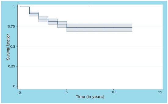
Figure 1. Kaplan–Meier estimates and 95% confidence limits of the survival function for the cryptocurrency data.

The survival outcomes of the levels of the variables can be compared graphically by using the Kaplan–Meier estimation of the survival function per group of covariate. The plots are displayed in Figure 2. The log-rank and Wilcoxon test statistics are summarized in Table 3.

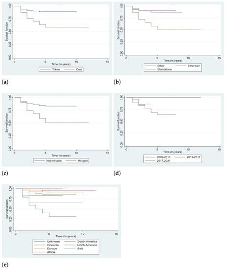
Figure 2. Plots of the Kaplan–Meier estimates of the survival function for levels of covariates from 2009 to 2021. (a) Type, (b) Blockchain, (c) Mining, (d) Series, (e) Region.

Table 3. Log-rank and Wilcoxon test statistics.

Variable	Log-Rank ${\mathit{\chi }}^2$ Test Statistic (p-Value)	Wilcoxon ${\mathit{\chi }}^2$ Test Statistic (p-Value)
Type	42.02 ($p<0.001$)	35.45 ($p<0.001$)
Blockchain	66.90 ($p<0.001$)	55.62 ($p<0.001$)
Mining	32.22 ($p<0.001$)	22.34 ($p<0.001$)
Series	13.10 (0.001)	8.04 (0.018)
Region	153.49 ($p<0.001$)	132.03 ($p<0.001$)

Figure 2a suggests that the survival outcome is significantly better for tokens as compared to coins $({\chi }^2=42.02;p<0.001)$. Figure 2b indicates a relatively better survival outcome for cryptocurrencies under Ethereum $({\chi }^2=66.90;p<0.001)$. Figure 2d suggests a significant high risk as a cryptocurrency is minable $({\chi }^2=32.22;p<0.001)$. Among the levels of the variable Series, cryptocurrencies released in the series 2009–2013 present significantly better survival outcomes $({\chi }^2=8.04;p=0.018)$ as Figure 2d indicates, this is the same for South American cryptocurrencies $({\chi }^2=132.03;p<0.001)$ as Figure 2e shows of the variable Region.

The log-rank test for comparison is suitable for comparing levels of covariates that obey the proportional hazard assumption (PHA); these are covariates Type, Blockchain and Mining for which the plots are approximately parallel. Wilcoxon test is suitable in comparing the levels of covariates Series and Region for which corresponding plots cross each other, leading to the violation of the PHA.

3. Results and Interpretation

3.1. Cox Proportional Hazards Model (CPHM)

Unlike Kaplan–Meier estimation, which treats one variable at a time, the the CPHM makes inference by considering several variables at a time.

Table 4 presents the estimated hazard ratios based on all the covariates.

Table 4. Cox Proportional hazards model for all covariates.

Covariate (Reference)	Level	Haz. Ratio	Std. Err.	z	P > z	95% Conf. Int.
Type (Token)	Coin	0.737	0.350	−0.640	0.521	[0.290; 1.872]
Blockchain (Other)	Ethereum	0.798	0.382	−0.470	0.638	[0.312; 2.041]
	Standalone	2.771	1.159	2.440	0.015	[1.221; 6.288]
Series (Series 1)	Series 2	$3.270$	$0.230$	2.840	0.671	$[1.452;3.215]$
	Series 3	$2.870$	0.952	1.450	0.424	[1.413; 3.624]
Mining (Not minable)	Minable	0.855	0.208	−0.640	0.520	[0.530; 1.378]
Region (Unknown)	South America	$0.091$	0.396	−0.562	0.741	[0.067; 0.201].
	Oceania	0.402	0.414	−0.880	0.377	[0.053; 3.031]
	North America	0.148	0.059	−4.800	$p<0.001$	[0.068; 0.322]
	Europe	0.230	0.068	−4.980	$p<0.001$	[0.129; 0.410]
	Asia	0.075	0.036	−5.370	$p<0.001$	[0.029; 0.193]
	Africa	0.755	0.554	−0.380	0.702	[0.179; 3.182]

The model suggests that the risk of death of cryptocurrencies under standalone blockchain is 2.771 (95% CI: 1.221; 6.288) times that of cryptocurrencies under the referral blockchain.

The significance for covariate Region is observed in North America, Europe and Asia. I all these regions the survival outcomes are better than the referral level. The CPHM suggests that the risk of death of cryptoccurrencies from unknown region is 6.757 (95% CI: [3.106; 14.706]) times that of cryptocurrencies based in North America. Such risk is 4.348 (95% CI: [2.439; 7.752]) times that of cryptocurrencies based in Europe and 13.333 (95% CI: [5.181; 34.483]) times that of cryptocurrencies based Asia.

3.2. Aalen Additive Hazards Model (AAHM)

Hosmer and Royston (2002) designed a STATA code based on an ado file for analysing survival data using the AAHM.

Figure 3a displays the cumulative parameter function with its 95% confidence limits for cryptocurrencies under Ethereum blockchain. The plot oscillates around the zero line, and the plot of 95% confidence limits are on either sides of the zero line. This indicates that the slope may be zero at some time value, and the risk of cryptocurrencies under Ethereum may not be significantly different from that of the referral group. The same AAHM results are observed for the crypto-coins (Figure 3c) and minable cryptocurrencies (Figure 3d).

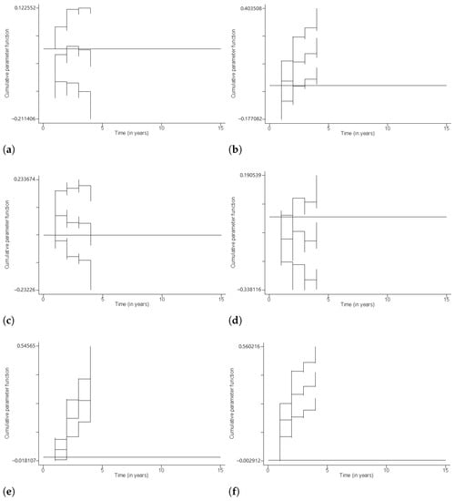
Figure 3. AAHM for levels of covariates Type, Blockchain, Mining and Series. (a) Ethereum, (b) Standalone, (c) Coin, (d) Minable, (e) Series 2 (2013–2017), (f) Series 3 (2017–2021).

Figure 3b indicates that the cumulative parameter function for cryptocurrencies under standalone blockchain is positive, and so is the major part of the 95% confidence limits. This suggests that the risk of such cryptocurrencies is higher than that of the referral group. The same observation occurred for cryptocurrencies released from the year 2013 as Figure 3e,f show.

Figure 4 gives the plots of the cumulative parameter functions and their 95% confidence limits for levels of the variable Region. The cumulative parameter functions with their 95% confidence limits are negative for levels South America (Figure 4a), North America (Figure 4c), Europe (Figure 4d) and Asia (Figure 4e). The pattern for level Oceania is negative together with the major parts of its confidence limits (Figure 4b). This suggests a relatively higher risk of cryptocurrencies of the referral region. The pattern for level Africa (Figure 4f) oscillates around the zero line, and the plot of 95% confidence limits are on either sides of the zero line. This indicates that the slope may be zero at some time value, and the risk of African cryptocurrencies may not be significantly different from that of the referral region.

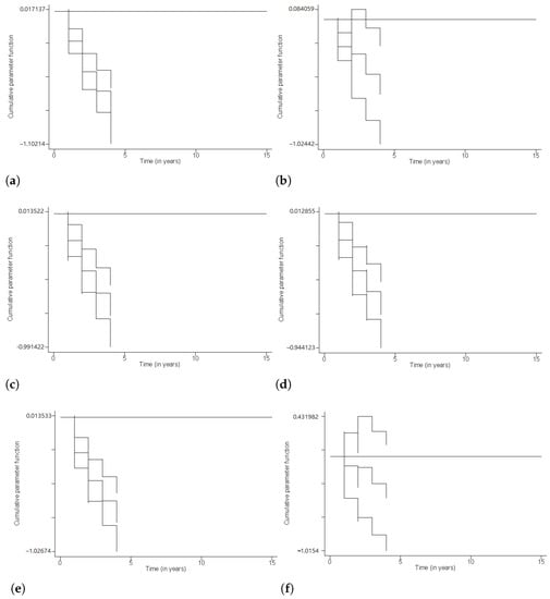
Figure 4. AAHM for levels of covariate Region. (a) South America, (b) Oceania, (c) North America, (d) Europe, (e) Asia, (f) Africa.

Table 5 displays the results of the test statistics of the AAHM for all the covariates using the four types of weights. All the tests are against the difference of the levels of covariate Mining. The test based on type 4 weights suggests the moderate evidence of difference of the levels of covariate Type and the overwhelming difference of levels of covariates Blockchain, Series and Region. The overwhelming difference for levels of covariate Series and some levels of covariate Region is also noticed by test 1, 2 and 3.

Table 5. Tests for significance of covariates.

		Test 1		Test 2		Test 3		Test 4
Covariate (Reference)	Level	z	P	z	P	z	P	z	P
Type (Token)	Coin	−0.477	0.634	0.004	0.997	−0.385	0.700	−2.229	0.026
Blockchain (Other)	Ethereum	−0.451	0.652	−0.437	0.662	−0.510	0.610	7.230	$p<0.001$
	Standalone	3.098	0.002	2.712	0.007	2.907	0.004	5.196	$p<0.001$
Series (Series 1)	Series 2	6.114	$p<0.001$	6.052	$p<0.001$	6.090	$p<0.001$	5.558	$p<0.001$
	Series 3	6.519	$p<0.001$	6.524	$p<0.001$	6.526	$p<0.001$	7.719	$p<0.001$
Mining (Not minable)	Minable	−0.324	0.746	−0.754	0.451	−0.448	0.654	0.990	0.322
Region (Unknown)	South America	−7.367	$p<0.001$	−7.784	$p<0.001$	−7.487	$p<0.001$	−7.365	$p<0.001$
	Oceania	−2.956	0.003	−2.935	0.003	−2.984	0.003	−7.153	$p<0.001$
	North America	−5.895	$p<0.001$	−6.312	$p<0.001$	−5.985	$p<0.001$	−6.110	$p<0.001$
	Europe	−5.332	$p<0.001$	−5.661	$p<0.001$	−5.403	$p<0.001$	−5.497	$p<0.001$
	Asia	−6.327	$p<0.001$	−6.837	$p<0.001$	−6.471	$p<0.001$	−6.353	$p<0.001$
	Africa	−1.468	0.142	−1.339	0.181	−1.418	0.156	−7.350	$p<0.001$

4. Conclusions

This paper used survival regression models for analysing the risk to death of the cryptocurrencies from 2009 to Q2 2021. The dataset is a sample of 500 cryptocurrencies for which a correct information on the covariates of interest were found. The exploration was conducted using the Kaplan–Meier estimation of the survival function.

The Cox Proportional Hazards Model (CPHM) also was used and suggested a relatively higher risk for cryptocurrencies under standalone blockchain. This result was also found by the plot of the survival functions of the levels of blockchain covariate. It was found by the CPHM that cryptocurrencies released in the series 2013–2017 are at a high risk as compared to those of 2009–2013 release. The CPHM also suggested that cryptocurrencies for which headquarters are unknown are at a relatively higher risk. The results of the Aalen Additive Hazards Models (AAHM) showed that unlike other covariates, the levels of covariate Mining are not significantly different.

Among more than 6000 active and inactive cryptocurrencies, this paper considered 500 cryptocurrencies for which the information on the variables of interest were easily found. The study still needs improvement by considering a relatively bigger sample size. Apart from considering a big sample in future research, re-sampling may also improve the measurement of the standard errors and then evaluate the accuracy of the results found in this paper.

References

- Aalen, Odd Olai, Ørnulf Borgan, and Håkon Kristian Gjessing. 2008. Survival and Event History Analysis. New York: Springer. [Google Scholar]
- Angela, Scott-Briggs. 2016. Ten types of digital currencies and how they work. Online Trading: Free Introductory eBook 2016: 24. [Google Scholar]
- Azimli, Asil. 2020. The impact of COVID-19 on the degree of dependence and structure of risk-return relationship: A quantile regression approach. Finance Research Letters 36: 101648. [Google Scholar] [CrossRef] [PubMed]
- Blundell-Wignall, Adrian. 2014. The Bitcoin question: Currency versus trust-less transfer technology. In OECD Working Papers on Finance, Insurance and Private Pensions, No 37. Paris: OECD Publishing. [Google Scholar]
- Breslow, Norman Edward. 1974. Covariance analysis of censored survival data. Biometrics 30: 89–99. [Google Scholar] [CrossRef] [PubMed]
- Chan, Stephen, Jeffrey Chu, Saralees Nadarajah, and Joerg Osterrieder. 2017. A statistical analysis of cryptocurrencies. Journal of Risk and Financial Management 10: 12. [Google Scholar] [CrossRef]
- Collet, David. 2003. Modeling Survival Data in Medical Research, 2nd ed. London: Chapman & Hall. [Google Scholar]
- Cox, David Roxbee. 1972. Regression models and life-tables (with discussion). Journal of the Royal Statistical Society, Series B 34: 187–220. [Google Scholar]
- De Best, Raynor. 2022. Number of cryptocurrencies worldwide. Statista 1: 2022. [Google Scholar]
- Efron, Bradley. 1977. The efficiency of Cox’s likelihood function for censored data. Journal of the American Statistical Association 72: 557–65. [Google Scholar] [CrossRef]
- Gatabazi, Paul, and Gaëtan Kabera. 2015. Survival Analysis and Its Stochastic Process Approach with Application to Diabetes Data. Johannesburg: University of Johannesburg. [Google Scholar]
- Gatabazi, Paul, Jules Clement Mba, and Edson Pindza. 2019a. Analysis of Cryptocurrencies Adoption Using Fractional Grey Lotka-Volterra Models. Johannesburg: University of Johannesburg. [Google Scholar]
- Gatabazi, Paul, Jules Clement Mba, and Edson Pindza. 2019b. Fractional Grey Lotka-Volterra model with application to cryptocurrencies adoption. Chaos: An Interdisciplinary Journal of Nonlinear Science 29: 073116. [Google Scholar] [CrossRef] [PubMed]
- Gatabazi, Paul, Jules Clement Mba, and Edson Pindza. 2019c. Modeling cryptocurrencies transaction counts using variable-order fractional grey Lotka-Volterra dynamical system. Chaos Solitons & Fractals 127: 283–90. [Google Scholar]
- Gatabazi, Paul, Jules Clement Mba, Edson Pindza, and Coenraad Labuschagne. 2019d. Grey Lotka-Volterra model with application to cryptocurrencies adoption. Chaos, Solitons & Fractals 122: 47–57. [Google Scholar]
- Gatabazi, Paul, Melesse Sileshi Fanta, and Shaun Ramroop. 2019e. Resampled Cox proportional hazards model for the infant mortality at the Kigali University Teaching Hospital. The Open Public Health Journal 12: 136–44. [Google Scholar] [CrossRef]
- Gatabazi, Paul, Melesse Sileshi Fanta, and Shaun Ramroop. 2018. Multiple events model for the infant mortality at Kigali University Teaching Hospital. The Open Public Health Journal 11: 464–73. [Google Scholar] [CrossRef][Green Version]
- Gatabazi, Paul, Melesse Sileshi Fanta, and Shaun Ramroop. 2020a. Comparison of three classes of marginal risk set model in predicting infant mortality among newborn babies at Kigali University Teaching Hospital, Rwanda, 2016. BMC Pediatrics 20: 62. [Google Scholar] [CrossRef] [PubMed]
- Gatabazi, Paul, Melesse Sileshi Fanta, and Shaun Ramroop. 2020b. Some Statistical Methods in Analysis of Single and Multiple Events with Application to Infant Mortality Data. KwaZulu Natal: University of KwaZulu Natal. [Google Scholar]
- Hendrickson, Joshua, Thomas Hogan, and William Luther. 2016. The political economy of Bitcoin. Economics Inquiry 54: 925–39. [Google Scholar] [CrossRef]
- Hosmer, David, Stanley Lemeshow, and Susanne May. 2008. Regression Modeling of Time-to-Event Data, 2nd ed. Haboken: John Wiley & Sons Inc. [Google Scholar]
- Hosmer, David, and Patrick Royston. 2002. Using Aalen’s linear hazards model to investigate time-varying effects in the proportional hazards regression model. The STATA Journal 2: 331–50. [Google Scholar] [CrossRef]
- Klein, John, and Melvin Moeschberger. 2003. Techniques for Censored and Truncated Data, 2nd ed. New York: Springer. [Google Scholar]
- Mba, Jules Clement, and Qing-Guo Wang. 2019. Multi-Period Portfolio Optimization: A Differential Evolution Copula-Based Approach. Johannesburg: University of Johannesburg. [Google Scholar]
- Mulaik, Stanley. 2009. Foundations of Factor Analysis, 2nd ed. Boca Raton: Chapman & Hall/CRC. [Google Scholar]
- Thul, Joaquin. 2021. El Salvador legalises Bitcoin: Hype or breakthrough? Infocus Macro Comment 9: 2021. [Google Scholar]
- Urquhart, Andrew. 2016. The inefficiency of Bitcoin. Economics Letters 148: 80–82. [Google Scholar] [CrossRef]
- Wu, Ke, Spencer Wheatley, and Didier Sornette. 2018. Classification of cryptocurrency coins and tokens by the dynamics of their market capitalizations. Royal Sosiety Open Science 5: 180381. [Google Scholar] [CrossRef]
- Xiao, Hui, Xiong Xiong, and Weiwei Chen. 2021. Introduction to the special issue on impact of COVID-19 and cryptocurrencies on the global fnancial market. Financial Innovation 7: 27. [Google Scholar] [CrossRef]
- Youssef, Manel, Khaled Mokni, and Ahdi Noomen Ajmi. 2021. Dynamic connectedness between stock markets in the presence of the COVID-19 pandemic: Does economic policy uncertainty matter? Financial Innovation 7: 13. [Google Scholar] [CrossRef] [PubMed]
Publisher’s Note: MDPI stays neutral with regard to jurisdictional claims in published maps and institutional affiliations. |
© 2022 by the authors. Licensee MDPI, Basel, Switzerland. This article is an open access article distributed under the terms and conditions of the Creative Commons Attribution (CC BY) license (https://creativecommons.org/licenses/by/4.0/).