Low-Thrust Transfer Method for Full Orbital Element Convergence Using J₂ Precession

Abstract

Low-thrust propulsion systems have become mainstream for Low Earth Orbit (LEO) satellites due to their superior propellant efficiency, yet conventional low-thrust transfer strategies suffer from high computational costs and failure to achieve full orbital element convergence. To address these drawbacks, this paper proposes a novel semi-analytical three-phase low-thrust transfer strategy that leverages $J_2$ gravitational precession to realize convergence of all orbital elements for circular orbits. The core of the method lies in the design of two symmetric thrust arcs and an intermediate coasting period that utilizes $J_2$ precession. By solving the resulting polynomial equation, the strategy achieves simultaneous controlled convergence of the Right Ascension of the Ascending Node (RAAN) and the argument of latitude (AOL). Simulation results demonstrate that the proposed method achieves significant fuel savings compared to direct transfer strategies, while simultaneously achieving superior computational speed. Extensive validation via 100,000 Monte Carlo simulations confirms the method’s scope of applicability, and the sufficient conditions for the existence of a solution are provided. It is further found that the proposed method is particularly well-suited for missions involving medium-to-high inclination orbits and large RAAN gaps, such as constellation deployment. In conclusion, this strategy provides a fuel-efficient and computationally fast solution for low-thrust transfer, establishing the basis for the operational management of future large-scale space systems equipped with low-thrust propulsion.

1. Introduction

Due to their very high effective exhaust velocity, low-thrust electric propulsion (EP) systems offer promising performance in propellant reduction, making them widely adopted in modern missions. With the exponential increase in the number of satellites being launched, an ever larger proportion of satellites are being equipped with EP systems. As of November 2025, more than 9500 of the over 12,000 operational LEO satellites are equipped with EP systems, including approximately 8800 Starlink satellites, about 650 OneWeb satellites, more than 100 Qianfan satellites, and more than 100 Xingwang satellites [1,2]. Mega-constellation satellites, numbering in the tens of thousands and characterized by the use of low-thrust EP systems, have come to dominate the LEO environment. In such constellations, deployment, configuration maintenance, reconfiguration, collision avoidance and deorbit all require low-thrust transfers performed by these satellites. The search for efficient low-thrust transfer strategies has therefore become a pressing problem.

Low-thrust transfer strategies have been extensively explored, typically formulating the problem as a time- or fuel-minimization task, where researchers derive near-optimal or optimal solutions using either direct or indirect methods. Direct methods convert the transfer problem into a discrete parameter optimization problem and solve it by Nonlinear Programming (NLP) algorithms, such as those demonstrated by Kluever and Oleseon [3], Gao [4], and Leomanni et al. [5]. Indirect methods convert the transfer problem into a Two-Point Boundary Value Problem (TPBVP) and solve it based on Pontryagin’s maximum principle (PMP), with representative techniques including the multihomotopic method [6] and heuristic approach [7]. Notably, combining the indirect method with the $J_2$ perturbation model can yield significant fuel savings for low-thrust transfer, as demonstrated by Cerf [8], who proposed a strategy for low-thrust transfer between circular orbits that exploits the natural $J_2$ precession to nullify the right ascension of the ascending node (RAAN) gap; subsequently, Shen [9] revisited Cerf’s approach, applying analytical optimization to derive an explicit, closed-form solution. Similarly, Wen et al. [10] expanded on Cerf’s study by addressing a control strategy incorporating yaw switch steering (YSS), further improving the fuel cost. Di Pasquale et al. [11] utilized an indirect approach, coupled with a genetic algorithm and Q-law algorithm, to reduce the time consumed for transfers exploiting $J_2$ precession. Huang et al. [12,13] achieved low-thrust rendezvous between circular and low-eccentricity orbits utilizing the natural RAAN drift caused by $J_2$ precession, but it still required the periodic switching of thrust on and off within each revolution. Dong et al. [14] achieved resonant control of low-thrust transfer with $J_2$ perturbation, but this required the thrust direction to be changed in real time. Similar methods utilizing $J_2$ precessions have also been applied to multi-target rendezvous [15] and debris removal missions [16].

However, the aforementioned methods are typically computationally expensive, with solving a single transfer case typically requiring tens of seconds to several minutes. This feature makes traditional optimization techniques unsuitable for contemporary mega-constellation scenarios, which may involve thousands of satellites and necessitate finding transfer solutions simultaneously. Consequently, there is a need to find analytical or semi-analytical strategies to improve computational efficiency. A common approach involves using closed-loop strategies based on current state variables, as exemplified by various studies [17,18,19]. Huang et al. developed a semi-analytical solution for efficient co-planar transfer with self-induced collision avoidance [20]. The authors’ team has introduced an artificial potential function-based method [21,22,23,24] that has been successfully validated in mega-constellation reconfiguration missions with proven Lyapunov stability.

Nevertheless, the preceding methods inherently require rapid adjustability of the thrust magnitude, thrust direction, satellite attitude, or frequent on/off switching, which often conflicts with the practical constraints imposed by most low-thrust propulsion systems and satellite attitude control in engineering applications; consequently, recent research has begun to shift toward finding analytical or semi-analytical strategies that utilize constant thrust. Kéchichianv [25] first calculated the analytic representations of optimal low-thrust transfer in circular orbit. McGarth and Macdonald [26] proposed an analytical method that incorporates both long- and short-term effects of $J_2$ perturbation based on constant thrust, and used it for constellation deployment [27]. Di Carlo and Vasile [28] further calculated analytical solutions for low-thrust orbit transfers, enabling variation in semi-major axes, inclination, and RAAN with $J_2$ perturbation. Despite the improved computational efficiency, these studies only guarantee the convergence of slow variables—semi-major axes, inclination, and RAAN—but fail to resolve the convergence issue of the phase variable, argument of latitude (AOL). Wang et al. [29] derived analytical approximations for the variation ranges of classical orbital elements under low-thrust conditions.

To address the problem of phase convergence, Lafleur and Apffel [30] proposed an analytical low-thrust strategy for in-plane phasing, but neglected the $J_2$ perturbation. Huang et al. [31] achieved the simultaneous adjustment of the RAAN and AOL by combining low-thrust with a pre-compensation for inclination and semi-major axes, using an analytical method and constant thrust. Hu et al. [32] introduced a semi-analytical three-stage strategy that achieved the convergence of all orbital elements for circular orbits; however, the method requires iterative computation of the time of flight, resulting in a relatively slow solution time of 40 s per case, and since it was only validated on a single case example, its utility cannot be guaranteed in more extensive maneuver scenarios. The authors’ recently proposed semi-analytical transfer method achieves a solution time of approximately half a second, and its application range has been validated through 100,000 Monte Carlo simulation cases [33,34]; however, this method treats the $J_2$ perturbation as a disturbing force and employs a direct maneuver to adjust the RAAN and AOL, resulting in relatively high fuel consumption.

To resolve the challenges posed by the preceding limitations, this paper develops a novel semi-analytical low-thrust transfer strategy that effectively utilizes $J_2$ precession to save fuel and guarantees the convergence of all orbital elements. The proposed methods are validated through extensive Monte Carlo simulations conducted over a substantial set of randomly generated cases, providing strong evidence for its broad practical applicability and lower fuel consumption compared to direct transfers. The remainder of the paper is organized as follows. In Section 2, the dynamical model is established. Section 3 defines the three-phase low-thrust maneuvering strategy. In Section 4, the effectiveness of the strategy is demonstrated through a specific example, and its applicability is validated by extensive numerical simulations. Section 5 discusses the existence conditions of the solutions of the proposed method and highlights its advantages and applicable missions. Finally, conclusions are drawn in Section 6.

2. Dynamical Model

Considering that the majority of operational Low Earth Orbit (LEO) satellites are currently operating in circular or near-circular orbits ($e\approx 0$), these trajectories are selected as the subject of this investigation. Consequently, the number of independent orbital elements required to define the orbit is reduced from $[a,e,i,\Omega ,\omega ,M]$ to $[a,i,\Omega ,u]$. The Lagrange planetary equations of mean orbital elements, considering only the long-term effects of $J_2$, reduce to [31]

$$\begin{array}{c}{\left({\displaystyle \frac{\mathrm{d}a}{\mathrm{d}t}}\right)}_{J_2}={\left({\displaystyle \frac{\mathrm{d}e}{\mathrm{d}t}}\right)}_{J_2}={\left({\displaystyle \frac{\mathrm{d}i}{\mathrm{d}t}}\right)}_{J_2}=0\end{array}$$

(1)

$$\begin{array}{c}{\left({\displaystyle \frac{\mathrm{d}\mathrm{\Omega }}{\mathrm{d}t}}\right)}_{J_2}=-{\displaystyle \frac{3n{J}_2{R}_e^2}{2a^2}}cosi\end{array}$$

(2)

$$\begin{array}{c}{\left({\displaystyle \frac{\mathrm{d}u}{\mathrm{d}t}}\right)}_{J_2}={\left({\displaystyle \frac{\mathrm{d}M}{\mathrm{d}t}}\right)}_{J_2}+{\left({\displaystyle \frac{\mathrm{d}\omega }{\mathrm{d}t}}\right)}_{J_2}=n+{\displaystyle \frac{3n{J}_2{R}_e^2}{2a^2}}\left(3-4{sin}^{2}i\right)\end{array}$$

(3)

where a is the semi-major axis, e is the eccentricity, i is the inclination, $\Omega$ is the RAAN, $\omega$ is the argument of perigee, M is the mean anomaly, $u=f+\omega$ is the AOL, $J_2$ is the coefficient of the second degree of the Earth’s gravitational zonal harmonic, and $R_e$ is the radius of the Earth. The mean motion n is defined as $n=\sqrt{\mu /a^3}$. For near-circular orbits, $f\approx M$; therefore, u can be approximated as $u\approx M+\omega$. Given that the propulsion acceleration is assumed to be small for a low-thrust system, the orbit is assumed to remain circular throughout the maneuver. This assumption is justified, as studies by Edelbaum [35] and Kechichian [36] indicate that the semi-major axis varies very slowly when the low-thrust acceleration is below ${10}^{-4}g$ (approximately $0.001{\mathrm{m}/\mathrm{s}}^2$). In such orbit evolution, the growth of eccentricity e is often regarded as a second-order small quantity; therefore, approximating the orbit as circular is acceptable for this analysis. The resulting equations of motion are thus [37]

$$\begin{array}{c}{\left({\displaystyle \frac{\mathrm{d}a}{\mathrm{d}t}}\right)}_{\mathrm{thrust}}={\displaystyle \frac{2}{n}}{a}_S\end{array}$$

(4)

$$\begin{array}{c}{\left({\displaystyle \frac{\mathrm{d}i}{\mathrm{d}t}}\right)}_{\mathrm{thrust}}={\displaystyle \frac{cosu}{na}}{a}_W\end{array}$$

(5)

$$\begin{array}{c}{\left({\displaystyle \frac{\mathrm{d}\Omega }{\mathrm{d}t}}\right)}_{\mathrm{thrust}}={\displaystyle \frac{sinu}{nasini}}{a}_W\end{array}$$

(6)

$$\begin{array}{c}{\left({\displaystyle \frac{\mathrm{d}u}{\mathrm{d}t}}\right)}_{\mathrm{thrust}}={\displaystyle \frac{2a_R}{na}}-{\displaystyle \frac{a_W}{na}}{\displaystyle \frac{sinu}{tani}}\end{array}$$

(7)

Here R is along the radius vector, W is along the orbit normal vector, and S is along the track (in orbit plane, normal to $R,W$) vector. $a_R,a_S,a_W$ are the along radius, track, and normal thrust accelerations. Equations (4)–(7) indicate that $a_W$ directly controls the RAAN and AOL, while $a_S$ directly controls the semi-major axis, thus indirectly controlling the RAAN and AOL.

3. Maneuver Strategy

The purpose of the maneuver is to make the orbital elements of the maneuvering satellite $\mathbf{z}={[a,i,\Omega ,u]}^{\mathrm{T}}$ converge to the reference value ${\mathbf{z}}_f={[a_f,i_f,{\Omega }_f,u_f]}^{\mathrm{T}}$, which can be characterized as a TPBVP, expressed as

$$\begin{array}{cc}\hfill & \dot{\mathbf{z}}={\mathbf{F}}_{\tilde{\mathbf{u}}}(\mathbf{z},\tilde{\mathbf{u}},t),{\dot{\mathbf{z}}}_f=\mathbf{F}({\mathbf{z}}_f,t)\hfill \\ \hfill & \mathbf{z}\left(t_0\right)={\mathbf{z}}_0={[a_0,i_0,{\Omega }_0,u_0]}^{\mathrm{T}},\hfill \\ \hfill & {\mathbf{z}}_f\left(t_0\right)={\mathbf{z}}_{f0}={[a_{f0},i_{f0},{\Omega }_{f0},u_{f0}]}^{\mathrm{T}}\hfill \\ \hfill & \mathbf{z}\left(t_0+\mathrm{ToF}\right)={\mathbf{z}}_f\left(t_0+\mathrm{ToF}\right)\hfill \\ \hfill & t\in \left[t_0,t_0+\mathrm{ToF}\right]\hfill \end{array}$$

(8)

Note that according to Equation (1), the values of $a_f$ and $i_f$ in the reference value can be considered constant throughout the entire process, i.e., $a_f\equiv a_{f0},i_f\equiv i_{f0}$. To achieve this goal, a low-thrust three-phase maneuvering strategy $\tilde{\mathbf{u}}$ is utilized, as illustrated in Figure 1.

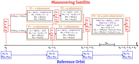
Figure 1. The diagram of the three-phase maneuvering strategy.

3.1. a-Adjustment and i-Adjustment: An Interchangeable Strategy

In Phases 1 and 2, a strategy is adopted where the adjustments of the semi-major axis a and the inclination i are interchangeable. We first address the adjustment of a assuming an arbitrary inclination i. An along-track acceleration $a_S$ is applied to maneuver the semi-major axis from $a_0$ to $a_f$:

$$a_S=\mathrm{sgn}(a_f-a_0)A$$

(9)

where A is the propulsive acceleration. $a_S$ takes a positive sign when the semi-major axis needs to increase and a negative sign when it decreases. The time duration and variation of orbital elements in a-adjustment are [31]

$$\begin{array}{cc}\hfill & t_a=\mathrm{sgn}(a_f-a_0){\displaystyle \frac{\sqrt{\mu }}{A}}\left({\displaystyle \frac{1}{\sqrt{a_0}}}-{\displaystyle \frac{1}{\sqrt{a_f}}}\right),\hfill \\ \hfill & \Delta a_a=a_f-a_0,\hfill \\ \hfill & \Delta i_a=0,\hfill \\ \hfill & \Delta {\Omega }_a\left(i\right)=\mathrm{sgn}(a_f-a_0)\left[{\Phi }_{\Omega }(a_f,i)-{\Phi }_{\Omega }\left(a_0,i\right)\right],\hfill \\ \hfill & \Delta u_a\left(i\right)=\mathrm{sgn}(a_f-a_0)\left[{\Phi }_u(a_f,i)-{\Phi }_u\left(a_0,i\right)\right]\hfill \end{array}$$

(10)

where

$$\begin{array}{cc}\hfill & {\Phi }_u\left(a,i\right)=-{\displaystyle \frac{\mu }{4A}}{a}^{-2}-{\displaystyle \frac{3\mu J_2{R}_E^2}{16A}}\left(3-4{sin}^{2}i\right)a^{-4}\hfill \\ \hfill & {\Phi }_{\Omega }\left(a,i\right)={\displaystyle \frac{3\mu J_2{R}_E^2}{16A}}cosi{a}^{-4}\hfill \end{array}$$

(11)

Next, we address the i-adjustment with the semi-major axis set to an arbitrary value a. The normal acceleration $a_W$ is applied to maneuver the inclination from $i_0$ to $i_f$, defined as [28]

$$a_W=\mathrm{sgn}(i_f-i_0)\mathrm{sgn}(cosu)A$$

(12)

$a_W$ takes a positive sign when the inclination needs to increase and a negative sign when it decreases. The time duration and variation of orbital elements in i-adjustment can be expressed as [34,38]

$$\begin{array}{cc}\hfill & t_i\left(a\right)={\displaystyle \frac{\pi |i_f-i_0|\sqrt{\mu }}{2A\sqrt{a}}},\hfill \\ \hfill & \Delta a_i=0,\hfill \\ \hfill & \Delta i_i=i_f-i_0,\hfill \\ \hfill & \Delta {\Omega }_i\left(a\right)=-{\displaystyle \frac{3\pi \mu J_2{R}_e^2(sin{i}_f-sin{i}_0)\mathrm{sgn}(i_f-i_0)}{4a^{4}A}},\hfill \\ \hfill & \Delta u_i\left(a\right)=\sqrt{{\displaystyle \frac{\mu }{a^3}}}{t}_i\hfill \end{array}$$

(13)

In Phases 1 and 2, the adjustments of the a and i are interchangeable in sequence. The values of t, $\Delta a$, $\Delta i$, $\Delta \Omega$, and $\Delta u$ for the two adjustment sequences ($a\to i$ and $i\to a$) across Phases 1 and 2 are presented in Figure 1. The presence of the $J_2$ perturbation causes the discrepancy between the maneuvering satellite’s RAAN and the reference value to evolve further following Phases 1 and 2. Consequently, selecting the appropriate adjustment sequence allows us to minimize the $\Delta \Omega$ required in Phase 3. Therefore, the absolute difference between the RAAN of the maneuvering satellite and the reference value at the end of Phase 2, $|\delta {\Omega }_2|=|{\Omega }_{f2}-{\Omega }_2|$, is adopted as the criterion to determine the actual execution order of adjusting a and i. The strategy yielding a smaller $|\delta {\Omega }_2|$ is chosen, as this facilitates a reduction in both fuel consumption and duration for Phase 3. $|\delta {\Omega }_2|$ under two adjustment sequences is defined as

$$\begin{array}{c}\hfill |\delta {\Omega }_2{|}_{ai}=\left|[{\Omega }_{f0}+{\dot{\Omega }}_f{t}_a+{\dot{\Omega }}_f{t}_i\left(a_f\right)]-[{\Omega }_0+\Delta {\Omega }_a\left(i_0\right)+\Delta {\Omega }_i\left(a_f\right)]\right|\\ \hfill |\delta {\Omega }_2{|}_{ia}=\left|\left[{\Omega }_{f0}+{\dot{\Omega }}_f{t}_i\left(a_0\right)+{\dot{\Omega }}_f{t}_a\right]-[{\Omega }_0+\Delta {\Omega }_i\left(a_0\right)+\Delta {\Omega }_a\left(i_f\right)]\right|\end{array}$$

(14)

Should $|\delta {\Omega }_2{|}_{ai}\le {\left|\delta {\Omega }_2\right|}_{ia}$, the sequence involving Phase 1 a-adjustment followed by Phase 2 i-adjustment is employed. Otherwise, the sequence of Phase 1 i-adjustment followed by Phase 2 a-adjustment is implemented.

It is particularly important to note that we need to clarify the influence of the two adjustment sequences ($a\to i$ and $i\to a$) on the fuel and time consumption in Phases 1 and 2. Considering that the expression for $t_a$ in Equation (10) is independent of the inclination term i, the time and fuel consumed for the a-adjustment (from $a_0$ to $a_f$) are identical, regardless of the chosen sequence. In addition, according to Equation (13), the time required for inclination adjustment, $t_i$, is inversely proportional to the square root of the semi-major axis a ($t_i\propto 1/\sqrt{a}$). Based on this relationship, we calculate that the relative difference in $t_i$ between orbits at altitudes of 300 km and 1200 km is approximately 6.5%. The velocity increment of inclination adjustment can also be estimated using $\Delta V_i=A·t_i$, indicating that approximately $200\mathrm{m}/\mathrm{s}$ is required to adjust the inclination by $1^{\circ }$. In typical low-thrust transfer missions, however, the required inclination change is usually limited to a few degrees. Consequently, the maximum time difference for the i-adjustment between the two sequences remains no more than $6.5\%$, corresponding to a maximum $\Delta V$ difference of approximately $15\mathrm{m}/\mathrm{s}$ per degree. This difference can be temporarily ignored, particularly in cases where the required RAAN adjustment in Phase 3 is substantial.

3.2. $\Omega$- and u-Joint Adjustment: A Three-Stage Strategy Using $J_2$ Precession

Following Phases 1 and 2, a and i reach their reference values ($a_2=a_f$ and $i_2=i_f$); Phase 3 utilizes a three-stage method based on [26]. Stage 1 of Phase 3 is an initial thrusting stage using constant along-track acceleration $a_s=\mathrm{sgn}\left(a_m-a_f\right)A$ to increase or decrease the satellite’s altitude relative to its initial orbit; this is followed by a Stage 2 of Phase 3, a coast arc at a constant altitude ($a_m$) for a total duration of $t_m$. Stage 3 of Phase 3 employs a thrust equal in magnitude but opposite in direction to Stage 1, over the same duration, to return the satellite to the initial $a_f$. The variation of maneuvering satellite’s a during Phase 3 is shown in Figure 2, where Figure 2a corresponds to the case $a_m>a_f$ and Figure 2b corresponds to $a_m<a_f$.

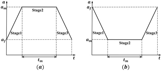
Figure 2. Variation of the semi-major axis a of the maneuvering satellite during the three-stage maneuver in Phase 3: (a) the case where $a_m>a_f$; and (b) the case where $a_m<a_f$.

The final objective of Phase 3 is to ensure that the maneuvering satellite’s RAAN $\Omega$ and AOL u equal their respective reference values, i.e., ${\Omega }_3={\Omega }_{f3}$ and $u_3=u_{f3}+2k\pi$, where $k\in \mathbb{Z}$. To achieve this goal, the altitude of the coast arc $a_m$ and duration $t_m$ must be determined; specifically, assuming the final inclination $i_f<{90}^{\circ }$ and the difference in RAAN ${\Omega }_{f2}>{\Omega }_2$ at the end of Phase 2, the satellite is required to perform an orbit increase for the RAAN phasing shown in Figure 2a (i.e., $a_m>a_f$), which leads to the following relationship based on Equation (10).

$$\begin{array}{c}{\Omega }_3={\Omega }_2+2\left[{\Phi }_{\Omega }\left(a_m\right)-{\Phi }_{\Omega }\left(a_f\right)\right]+{\dot{\Omega }}_m{t}_m\end{array}$$

(15)

$$\begin{array}{c}{u}_3=u_2+2\left[{\Phi }_u\left(a_m\right)-{\Phi }_u\left(a_f\right)\right]+n_m{t}_m\end{array}$$

(16)

and

$$\begin{array}{c}{\Omega }_{f3}={\Omega }_{f2}+{\dot{\Omega }}_f\left[{\displaystyle \frac{2\sqrt{\mu }}{A}}\left({\displaystyle \frac{1}{\sqrt{a_f}}}-{\displaystyle \frac{1}{\sqrt{a_m}}}\right)+t_m\right]\end{array}$$

(17)

$$\begin{array}{c}{u}_{f3}=u_{f2}+n_f\left[{\displaystyle \frac{2\sqrt{\mu }}{A}}\left({\displaystyle \frac{1}{\sqrt{a_f}}}-{\displaystyle \frac{1}{\sqrt{a_m}}}\right)+t_m\right]\end{array}$$

(18)

Using Equations (15) and (17) and condition ${\Omega }_3={\Omega }_{f3}$, $t_m$ can be expressed as

$$t_m={\displaystyle \frac{({\Omega }_{f2}-{\Omega }_2)-2\left[{\Phi }_{\Omega }\left(a_m\right)-{\Phi }_{\Omega }\left(a_f\right)\right]-(2\sqrt{\mu }/A)(a_f^{-0.5}-a_m^{-0.5}){\dot{\Omega }}_f}{{\dot{\Omega }}_m-{\dot{\Omega }}_f}}$$

(19)

Substituting the above $t_m$ expression into Equations (16) and (18), and utilizing the condition $u_3=u_{f3}+2k\pi ,k\in \mathbb{Z}$, the following equation containing only $a_m$ as the unknown can be obtained:

$$u_{f2}-u_2+2k\pi =2\left[{\Phi }_u\left(a_m\right)-{\Phi }_u\left(a_f\right)\right]-{\displaystyle \frac{2\sqrt{\mu }}{A}}(a_f^{-0.5}-a_m^{-0.5}){\dot{\Omega }}_f+(n_m-n_f)t_m,k\in \mathbb{Z}$$

(20)

Here, since the inclination adjustment is complete, the primitive function $\Phi$ is denoted as $\Phi (a,i)=\Phi \left(a\right)$. After simplifying the aforementioned equation by finding a common denominator, it can be reformulated as a polynomial equation in terms of $a_m^{-0.5}$. Recognizing that the degree of this polynomial equation exceeds five, it does not possess a closed-form (algebraic) solution. Consequently, a numerical solution must be determined using well-established methods such as Newton iteration. It should also be noted that, Equation (20) does not guarantee a solution for $a_m$; thus, to obtain the solvability condition, we denote the right-hand side of the equation as a continuous function of $a_m$, $g\left(a_m\right)$, and investigate its range, where a solution to Equation (20) exists if and only if $u_{f2}-u_2+2k\pi$ falls within the range of $g\left(a_m\right)$. Here we have

$$\begin{array}{cc}\hfill & g\left(a_m\right)=2\left[{\Phi }_u\left(a_m\right)-{\Phi }_u\left(a_f\right)\right]-{\displaystyle \frac{2\sqrt{\mu }}{A}}(a_f^{-0.5}-a_m^{-0.5}){\dot{\Omega }}_f\hfill \\ \hfill & +\left({\displaystyle \frac{n_m-n_f}{{\dot{\Omega }}_m-{\dot{\Omega }}_f}}\right)\left\{({\Omega }_{f2}-{\Omega }_2)-2\left[{\Phi }_{\Omega }\left(a_m\right)-{\Phi }_{\Omega }\left(a_f\right)\right]-{\displaystyle \frac{2\sqrt{\mu }}{A}}(a_f^{-0.5}-a_m^{-0.5}){\dot{\Omega }}_f\right\}\hfill \end{array}$$

(21)

To this end, we first consider the case where $a_m$ approaches its lower limit, shown in Figure 3a. Noting that although $a_m$ can infinitely approach $a_f$, causing $t_m$ to tend toward infinity, the function $g\left(a_m\right)$ remains finite and can be determined via L’Hôpital’s rule as

$$\begin{array}{cc}\hfill & g\left(a_f^{+}\right)=\underset{a_m\to a_f^{+}}{lim}g\left(a_m\right)=\underset{a_m\to a_f^{+}}{lim}\left[({\Omega }_{f2}-{\Omega }_2)\left({\displaystyle \frac{n_m-n_f}{{\dot{\Omega }}_m-{\dot{\Omega }}_f}}\right)\right]\hfill \\ \hfill & =({\Omega }_{f2}-{\Omega }_2)\underset{a_m\to a_f^{+}}{lim}\left[{\displaystyle \frac{\sqrt{\mu }(a_m^{-1.5}-a_f^{-1.5})+1.5\sqrt{\mu }{J}_2{R}_e^2(3-4{sin}^2{i}_f)(a_m^{-3.5}-a_f^{-3.5})}{-1.5\sqrt{\mu }{J}_2{R}_e^{2}cos{i}_f(a_m^{-3.5}-a_f^{-3.5})}}\right]\hfill \\ \hfill & =-({\Omega }_{f2}-{\Omega }_2)\left({\displaystyle \frac{2a_f^2}{7J_2{R}_e^{2}cos{i}_f}}+{\displaystyle \frac{3-4{sin}^2{i}_f}{cos{i}_f}}\right)\hfill \end{array}$$

(22)

Second, we consider the upper limit of $a_m$, where it is readily shown that $a_m$ attains its maximum value $a_m^{max}$ when $t_m=0$, shown in Figure 3b. This corresponds to the numerator of the right-hand side of Equation (19) being zero, which is

$$({\Omega }_{f2}-{\Omega }_2)+{\displaystyle \frac{3\mu J_2{R}_E^2}{8A}}cos{i}_f(a_m^{-4}-a_f^{-4})-{\displaystyle \frac{3\sqrt{\mu }{J}_2{R}_e^2}{A}}cos{i}_f(a_f^{-0.5}-a_m^{-0.5})a_f^{-3.5}=0$$

(23)

The equation above is an eighth-order monotonic polynomial equation with respect to $a_m^{-0.5}$, the solution of which provides $a_m^{max}$.

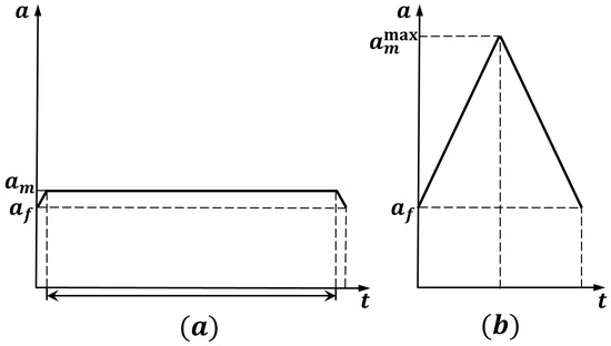
Figure 3. Variation in the semi-major axis a during Phase 3 when $a_m$ takes its boundary values: (a) the lower limit case where $a_m\to a_f^{+}$ and $t_m\to \infty$; and (b) the upper limit case where $a_m$ attains its maximum value, $a_m^{max}$, and $t_m=0$.

Furthermore, to obtain the range of $g\left(a_m\right)$, $g_{\mathrm{up}}$ and $g_{\mathrm{low}}$ are defined as follows:

$$\begin{array}{c}\hfill g_{\mathrm{up}}=max\left[g\left(a_f^{+}\right),g\left(a_m^{max}\right)\right],\\ \hfill g_{\mathrm{low}}=min\left[g\left(a_f^{+}\right),g\left(a_m^{max}\right)\right]\end{array}$$

(24)

When $a_m\in (a_f,a_m^{max}]$, the interval $(g_{\mathrm{low}},g_{\mathrm{up}}]$ is a subset of the range of $g\left(a_m\right)$; since $g\left(a_m\right)$ is a continuous function, we can consequently assert that for any $\delta u\in (g_{\mathrm{low}},g_{\mathrm{up}}]$, the equation $g\left(a_m\right)=\delta u$ guarantees a solution within the interval $a_m\in (a_f,a_m^{max}]$. In summary, we can therefore state the sufficient condition for the existence of solutions for $a_m$ and $t_m$:

$$\exists k\in \mathbb{Z},\mathrm{s}.\mathrm{t}.u_{f2}-u_2+2k\pi \in [g_{\mathrm{low}},g_{\mathrm{up}}]$$

(25)

Specifically, we define the interval length as $L=g_{\mathrm{up}}-g_{\mathrm{low}}$; it is evident that when $L\ge 2\pi$, solutions for $a_m$ and $t_m$ always exist, regardless of the values of $u_2$ and $u_{\mathrm{ref}2}$.

After solving for the semi-major axis $a_m$ and the duration $t_m$, the total maneuver duration or time of flight $\mathrm{ToF}$ of the entire maneuvering process are obtained by integrating the results from Section 3.1 and Section 3.2 as

$$\mathrm{ToF}=t_1+t_2+{\displaystyle \frac{2\sqrt{\mu }}{A}}\left|{\displaystyle \frac{1}{\sqrt{a_f}}}-{\displaystyle \frac{1}{\sqrt{a_m}}}\right|+t_m$$

(26)

3.3. Atmospheric Drag Compensation

In particular, during the maneuver, the satellite requires thrust aligned with the velocity vector to counteract the effects of atmospheric drag. Assuming a static atmosphere, the resulting acceleration due to atmospheric drag is given by

$$A_{\mathrm{atm}}={\displaystyle \frac{1}{2}}{\displaystyle \frac{C_{D}S}{m}}\rho v^2$$

(27)

where $\rho$ is the mass density of the atmosphere at the satellite’s position, $v=\sqrt{\mu /a}$ is the satellite velocity, $C_D$ is the drag coefficient, S is the cross-sectional area of the satellite perpendicular to its direction of motion, and m is the satellite mass. The exponential model is used to calculate the atmospheric density:

$$\rho ={\rho }_{\mathrm{ref}}\exp \left(-{\displaystyle \frac{h-h_{\mathrm{ref}}}{H}}\right)$$

(28)

where ${\rho }_{\mathrm{ref}}$ is the air density at reference height, and H is the effective height of atmosphere [39]. In the case of a circular orbit, the altitude above the Earth’s surface $h=a-R_e$.

Atmospheric drag primarily affects the semi-major axis and the AOL, leading to orbital decay and phasing errors. In practice, accurately quantifying the effect of atmospheric drag is nontrivial; therefore, we treat it as a perturbation. In particular, we compensate for the drag-induced acceleration by applying a small additional thrust along the S direction. Once the acceleration caused by atmospheric drag has been calculated for a fixed height using Equation (27), the velocity increment to compensate for the atmospheric drag during time length t is $\Delta V_{\mathrm{atm}}=A_{\mathrm{atm}}t$. Here t can be replaced by inclination adjustment time of i-adjustment $t_i$ or coasting time of Phase 3 Stage 2 $t_m$. For the a-adjustment and Phase 3 Stages 1 and 3, the semi-major axis a gradually increases or decreases linearly with time, leading to a corresponding change in atmospheric drag. By integrating the atmospheric drag acceleration over time during this process, the velocity increment that needs to be compensated when using along-track thrust to raise the semi-major axis from a to $a^{\prime }$ is given by

$$\Delta V_{\mathrm{atm}}={\varphi }_{\Delta V_{\mathrm{atm}}}{|}_a^{a^{\prime }}={\varphi }_{\Delta V_{\mathrm{atm}}}\left(a^{\prime }\right)-{\varphi }_{\Delta V_{\mathrm{atm}}}\left(a\right)$$

(29)

where ${\varphi }_{\Delta V_{\mathrm{atm}}}$ is the primitive function to compensate for atmospheric drag, given as

$$\begin{array}{cc}\hfill & {\varphi }_{\Delta V_{\mathrm{atm}}}\left(a\right)=\int A_{\mathrm{atm}}\mathrm{d}t=\int A_{\mathrm{atm}}{\displaystyle \frac{n}{2A}}\mathrm{d}a\hfill \\ \hfill & =\int {\displaystyle \frac{C_{D}S{\mu }^{\frac{3}{2}}}{4mA}}{\rho }_{\mathrm{ref}}exp\left({\displaystyle \frac{R_e+h_{\mathrm{ref}}}{H}}\right)\left[a^{-{\displaystyle \frac{5}{2}}}-{\displaystyle \frac{3}{4}}{J}_2{R}_E^2\left(3{sin}^{2}i-2\right)a^{-{\displaystyle \frac{7}{2}}}\right]exp\left(-{\displaystyle \frac{a}{H}}\right)\mathrm{d}a\hfill \\ \hfill & ={\displaystyle \frac{1}{4}}{\displaystyle \frac{C_{D}S{\mu }^{\frac{3}{2}}}{mA}}{\rho }_{\mathrm{ref}}exp\left({\displaystyle \frac{R_e+h_{\mathrm{ref}}}{H}}\right)\left[-H^{-{\displaystyle \frac{3}{2}}}\Gamma \left(-{\displaystyle \frac{3}{2}},{\displaystyle \frac{a}{H}}\right)+{\displaystyle \frac{3}{4}}{J}_2{R}_e^2\left(3{sin}^{2}i-2\right)H^{-{\displaystyle \frac{7}{2}}}\Gamma \left(-{\displaystyle \frac{7}{2}},{\displaystyle \frac{a}{H}}\right)\right]\hfill \end{array}$$

(30)

$\Gamma (s,x)$ is the upper incomplete Gamma function, defined by

$$\Gamma (s,x)={\int }_x^{\infty }{t}^{s-1}{e}^{-t}\mathrm{d}t$$

(31)

The total velocity increment $\Delta V_{\mathrm{total}}$ of the entire maneuvering process therefore is

$$\Delta V_{\mathrm{total}}=A·\mathrm{ToF}+A_{\mathrm{atm}}^{a_0}{t}_1+{\left|{\varphi }_{\Delta V_{\mathrm{atm}}}\right|}_{a_0}^{a_f}|+2{\left|{\varphi }_{\Delta V_{\mathrm{atm}}}\right|}_{a_f}^{a_m}|+A_{\mathrm{atm}}^{a_m}{t}_m$$

(32)

4. Simulation and Results

To conduct numerical simulations and validate the method’s feasibility, the initial step requires determining the appropriate satellite parameters and geographical constants, as shown in Table 1. The selected satellite parameters, featuring a thrust of 100 mN, a mass of 500 kg, and a specific impulse of 3000 s, were established by comparison with the Deep Space 1 (DS1) mission. For contextual reference, the DS1 spacecraft utilized the NSTAR ion thruster, with a thrust of 92 mN, a mass of 490 kg, and a specific impulse of 3280 s, carrying 83 kg of Xenon propellant [40], designed and fabricated by Hughes Electron Dynamics, Torrance, California, USA. Assuming the low-thrust acceleration remains constant during the maneuver, $A=F/m=2\times {10}^{-4}{\mathrm{m}/\mathrm{s}}^2$. The relationship between the total consumed fuel mass $\Delta m$ and the total velocity change $\Delta V$ is given by [24]

$$\Delta m={\displaystyle \frac{m\Delta V}{g{I}_{sp}}}$$

(33)

where g is the gravitational acceleration, $I_{sp}$ is the specific impulse, and $\Delta V$ can be calculated by Equation (32). This formula allows for the calculation of the total fuel mass consumed during the maneuver, $\Delta m$. In practice, the fuel consumption during the maneuver is typically minimal, generally not exceeding $5\%$ of the satellite’s total mass. The atmospheric density is modeled using CIRA-72 for 25–500 km and CIRA-72 with exospheric temperature $T_{\infty }=1000\mathrm{K}$ for 500–1000 km [41]. The reference density ${\rho }_{\mathrm{ref}}$ and the scale height H for different altitude intervals are provided in [37]. If the satellite crosses multiple altitude intervals during its maneuver, the integration can be performed separately for each interval. With these parameters established, the numerical simulation can now be performed. All simulation scenarios were run on an Intel Ultra 9-275HX processor with 24 cores @ 2.7 GHz using Matlab^® R2024b. Specifically, Equations (20) and (23) are solved using the modified Newton–Raphson method.

Table 1. Satellite parameters and geographical constants.

Constant	Value
Mass m	500 kg
Thrust F	100 mN
Specific Impulse $I_{sp}$	3000 s
Surface Area S	$5{\mathrm{m}}^2$
Drag Coefficient $C_D$	2.25
Earth Radius $R_e$	6378.137 km
Gravitational acceleration g	$9.80665\mathrm{m}/{\mathrm{s}}^2$
Earth gravitational constant $\mu$	398,600.4418 $\times {10}^9{\mathrm{m}}^3/{\mathrm{s}}^2$
$J_2$ constant	$1.0827\times {10}^{-3}$
Atmospheric model	CIRA-72

4.1. Performance of the Proposed Strategy

A comprehensive case study was conducted as an initial step to investigate the performance of the proposed strategy, quantitatively comparing the results of the three-phase maneuvering strategy using $J_2$ precession with those derived from the direct transfer method. The initial orbital elements of the maneuvering satellite and the reference orbit are provided in Table 2.

Table 2. Orbital elements for simulation.

Orbit	a, km	${\mathit{i},}^{\circ }$	${\mathbf{\Omega },}^{\circ }$	${\mathit{u},}^{\circ }$
Maneuvering ${\mathbf{z}}_0$	6878.137 km	${52}^{\circ }$	$0^{\circ }$	${10}^{\circ }$
Reference ${\mathbf{z}}_{f0}$	6978.137 km	${54}^{\circ }$	${15}^{\circ }$	${80}^{\circ }$

First, to verify the practical utility of the proposed method in an engineering context, a consistency check is conducted by comparing the analytical model with the results of numerical evolution. The high-fidelity numerical model employed for validation propagates the satellite state using Brouwer–Lyddane mean elements. The integration is performed via the Runge–Kutta–Fehlberg 7th-order and 8th-degree method with fractional step control, maintaining an absolute error tolerance of ${10}^{-10}$ and a relative tolerance of ${10}^{-13}$. The perturbation model accounts for a 10th-degree and 10th-order Earth gravity field, as well as the third-body gravitational effects from the Sun and Moon. Figure 4 presents the spatial separation between the satellite positions derived from the analytical and numerical models throughout the maneuver. Across different phases, this distance displays periodic oscillations, largely stemming from short-period perturbations triggered by the $J_2$ zonal harmonic and higher-order gravity terms, which are not explicitly modeled in the analytical framework. Over a propagation period exceeding 100 days, the maximum deviation reaches 174.92 km. These findings indicate that the developed analytical model maintains a substantial level of consistency with the high-fidelity numerical simulation regarding orbital maneuver predictions, further confirming the precision and robustness of the proposed analytical method.

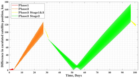
Figure 4. Distance between satellite positions as calculated by analytical and numerical solutions.

The control results obtained from the proposed three-phase method were then evaluated. According to the criterion defined in Section 3.1, the residual RAAN differences were $|\delta {\Omega }_2{|}_{ai}=18.{50}^{\circ }$ and $|\delta {\Omega }_2{|}_{ia}=23.{18}^{\circ }$, respectively. As the $a\to i$ sequence yields the smaller difference, the sequence of Phase 1 a-adjustment followed by Phase 2 i-adjustment is selected for the present case. In the simulation, the maneuver was completed within a total duration of $\mathrm{ToF}=100.68\mathrm{days}$, requiring a total velocity increment of $\Delta V_{\mathrm{total}}=607.29\mathrm{m}/\mathrm{s}$ (including atmospheric friction compensation $\Delta V_{\mathrm{atm}}=0.37\mathrm{m}/\mathrm{s}$), which corresponds to a fuel consumption of 10.32 kg. The durations for each specific phase were: 3.17 days for the semi-major axis adjustment (Phase 1), 23.97 days for the inclination adjustment (Phase 2), and 73.54 days for the joint adjustment of $\Omega$ and u (Phase 3); specifically within Phase 3, Stages 1 and 3 required 3.99 days, while the coasting arc in Stage 2 lasted for 65.56 days. The required $\Delta V$ values for the three phases were 54.81, 414.40, and 138.09 m/s, respectively.

Figure 5 illustrates the control inputs during the maneuver process, specifically the propulsive acceleration values in the $S, R,$ and W directions. It can be observed that in Phase 1 and Stage 1 of Phase 3, $a_S=A$ is applied to increase the semi-major axis, while $a_S=-A$ is required in Stage 3 of Phase 3 to decrease it. In Phase 2, $a_W=\pm A$ is utilized to achieve the inclination increment. No thrust is required throughout Stage 2 of Phase 3. $a_R$ remains zero for the entire process. Figure 6 illustrates the initial and final states of the maneuvering satellite and reference orbit. Despite their initial separation in distinct orbital elements, the satellites converge to a state of near-perfect collocation after the execution of the maneuver. The trajectory evolution of the maneuvering satellite is presented in Figure 7. The trajectories corresponding to the three phases are plotted using distinct colors: specifically, Phase 1 is represented by red, Phase 2 by orange, and Phase 3 is distinguished by yellow for Stages 1 and 3, and green for Stage 2, respectively.

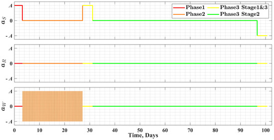
Figure 5. Control input $a_S, a_R, a_W$ during the maneuvering process; It is noted that $a_W$ needs to switch direction twice per orbital period in Phase 2, thus appearing very dense.

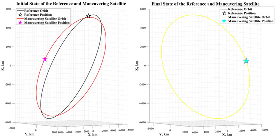
Figure 6. The initial and final trajectory of the maneuvering and reference satellite. It should be noted that the maneuvering satellite and the reference orbit in the right panel almost coincide.

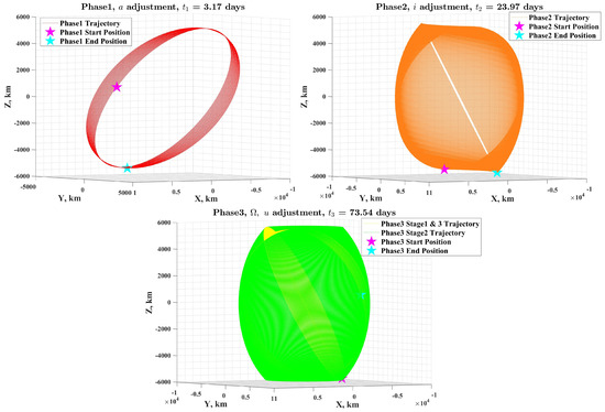
Figure 7. Trajectory of the maneuvering satellite during the three phases.

The time histories of the orbital elements of the maneuvering satellite and reference orbit during the maneuver are presented in Figure 8. Phases 1–3 are also marked with the same colors as in the previous figures. Specifically, to provide a more intuitive illustration, the time histories of ${\Omega }_f-\Omega$ and $u_f-u$ during the maneuver are plotted in Figure 9. Phase 3 Stage 2 (in green) corresponds to the segment where $J_2$ precession is used to drive the convergence of $\Omega$ and u. It can be observed that the orbital elements of the maneuvering satellite eventually converge to the reference values. At the final time, the deviation in the semi-major axis, $|a_3-a_{f3}|$, is less than $1\mathrm{m}$, the inclination error, $|i_3-i_{f3}|=0.{002}^{\circ }$, and both the RAAN error, $|{\Omega }_{f3}-{\Omega }_3|$, and the AOL error, $|u_{f3}-u_3|$, are less than ${10}^{-6\circ }$. Therefore, in this case, the proposed method achieves full orbital element convergence in $[a,i,\Omega ,u]$.

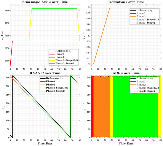
Figure 8. Orbital elements $a,i,\Omega ,u$ over time during maneuver.

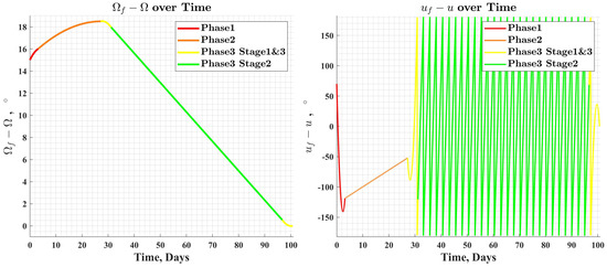
Figure 9. ${\Omega }_f-\Omega$ and $u_f-u$ over time during maneuver.

Furthermore, to facilitate a quantitative evaluation of computational speed and mission costs, the proposed method was benchmarked against a comparison method. In this baseline method, the adjustments of a and i are identical to the proposed method, but the adjustments of $\Omega$ and u employ the direct transfer method from our prior work [34]. The orbital elements used for the simulation remained identical to those presented in Table 2, and the CPU performance was also kept consistent. For the exact same case study, the proposed three-phase method achieved a solving time of 0.1 s, which is approximately one-fifth of the time required by the original method.

Consequently, since the strategies employed in the first two phases are the same, our primary comparison focuses on the fuel and time consumption of Phase 3. As illustrated in Table 3, the proposed method holds a significant advantage in terms of both mission time and fuel consumption due to its utilization of $J_2$ precession; the required duration for $\Omega$ and u adjustment was reduced by more than half, and the necessary $\Delta V$ was less than 5% of that required by the direct method. For the case study specified in Table 3, the proposed method achieves lower propellant consumption and shorter transfer time, thereby exhibiting superior performance. Particularly, for the adjustment of RAAN $\Omega$ and AOL u, this strategy eliminates the need for the ${180}^{\circ }$ thrust reversal required by the direct method every lap. Instead, it only necessitates continuous burning using constant along-track thrust followed by waiting during the coast arc, thereby making it more applicable in engineering.

Table 3. Time and $\Delta V$ cost and computation time comparison.

	Proposed Method	Direct Transfer Method in [34] for $\mathbf{\Omega },\mathit{u}$ Adjustment
ToF, days	100.68	208.10
$\Delta V$, m/s	607.29	3597.63
t for $\Omega ,u$ adjustment, days	73.54	180.96
$\Delta V$ for $\Omega ,u$ adjustment, m/s	138.09	3128.42
Computation Time, s	≈0.1 s	≈0.5 s

It should also be noted that the strategy proposed in this study is suboptimal by design (sequential) when compared to a fully optimal transfer. Compared with classical optimization methods, the proposed approach may require a longer transfer time. However, the best of existing studies show that solving the fully optimal transfer using indirect methods requires a computation time ranging from approximately 10 s to 1 min [6]. Therefore, the proposed method trades optimality for computational efficiency, yielding a performance gain of at least 100 times compared to the existing indirect methods. This significant speed improvement enables its application to the parallel computation of low-thrust transfers for mega-constellations comprising thousands of satellites, for which the computational cost using previous methods would be unacceptable.

4.2. General Applicability of the Proposed Strategy

To further assess the applicability of the proposed three-phase maneuver method, comprehensive validation was carried out utilizing Monte Carlo simulations. This extensive testing regime incorporated diverse initial conditions to confirm the method’s robustness and reliability. In total, 100,000 maneuver scenarios were stochastically generated, with the successful determination of $a_m$ and $t_m$ serving as the criterion for a successful solution. The initial orbital elements for these scenarios were sampled within the boundaries defined in Table 4.

Table 4. Orbital element range for Monte Carlo simulation.

Orbit	a, km	${\mathit{i},}^{\circ }$	${\mathbf{\Omega },}^{\circ }$	${\mathit{u},}^{\circ }$
Maneuvering ${\mathbf{z}}_0$	$R_e$ + [300 km, 1200 km]	$[{30}^{\circ },{80}^{\circ }]$	$[0^{\circ },{360}^{\circ })$	$[0^{\circ },{360}^{\circ })$
Reference ${\mathbf{z}}_{f0}$	$a_0$ + [−100 km, 100 km]	$i_0+[-3^{\circ },3^{\circ }]$	${\Omega }_0+[-{30}^{\circ },{30}^{\circ }]$	$[0^{\circ },{360}^{\circ })$

The entire simulation was processed in a total time of 10,457 s, yielding an average computational time of approximately 0.1 s per case, thus demonstrating exceptionally high computational efficiency. Among the 100,000 simulated scenarios, 73,658 cases satisfied the constraints on $u_{f2}-u_2$ and ${\Omega }_{f2}-{\Omega }_2$ as defined by Equation (25), all of which yielded feasible solutions. In contrast, 26,342 cases failed to meet the conditions in Equation (25). Within this subset, 15 cases were solvable, while the remaining 26,327 cases were unsolvable. These results demonstrate that the all the failed cases fall within the expectations established by the existence conditions in Equation (25). Nevertheless, a few exceptional cases exist where solutions are obtainable despite violating Equation (25). This phenomenon may be attributed to the non-monotonic behavior of $g\left(a\right)$ with respect to $a_m$ under these specific conditions, leading to the following possibilities:

$$\exists a_m\in (a_f,a_m^{max}],\mathrm{s}.\mathrm{t}.g\left(a_m\right)\notin [g_{\mathrm{low}},g_{\mathrm{up}}]$$

(34)

This outcome indicates that, within the established boundaries, the proposed method is applicable to approximately 73.67% of the scenarios defined in Table 4. The simulation results further indicate that the sufficient condition in Equation (25) is very close to being both necessary and sufficient; thus, in most cases, it can be used as an effective equivalence criterion for determining whether a feasible solution exists. The specific conditions under which the proposed method yields a solution will be further addressed in Section 5.

5. Discussion

As demonstrated in Section 4.2, the three-phase strategy does not always have a solution for all combinations of orbital elements. Therefore, the following question need to be addressed: under what conditions can the proposed method be applied? Equation (25) provides the sufficient condition for the existence of solutions for $a_m$ and $t_m$, indicating that a solution always exists when $L\ge 2\pi$. From Equations (22) and (23), it can be seen that L depends on the propulsive acceleration A, reference semi-major axis $a_f$, inclination $i_f$, maneuver, and the difference in RAAN of the reference satellite at the end of Phase 2, ${\Omega }_{f2}-{\Omega }_2$. Given that the propulsive acceleration A is fixed and the inclination $i_f$ typically changes little, we focus on investigating the impact of $a_f$ and ${\Omega }_{f2}-{\Omega }_2$ on L. To this end, we plot the contour of $L/2\pi$ as a function of $a_f$ and ${\Omega }_{f2}-{\Omega }_2$ for $A=2\times {10}^{-4}{\mathrm{m}/\mathrm{s}}^2$ and inclination $i={30}^{\circ }$–${80}^{\circ }$, shown in Figure 10. Specifically, the range for $a_f$ is $[R_e+300\mathrm{km},R_e+1200\mathrm{km}]$, and the range for the RAAN difference is ${\Omega }_{f2}-{\Omega }_2$, is $[0^{\circ },{30}^{\circ }]$. Due to symmetry, we only plotted the cases where ${\Omega }_{f2}-{\Omega }_2$ is positive; the corresponding negative values can be realized by setting $a_m<a_f$ in Phase 3 Stage 2 to implement RAAN waiting.

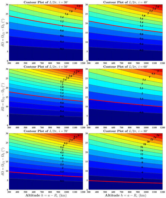
Figure 10. Contour plot of $L/\left(2\pi \right)$ for final inclinations $i_f=\{{30}^{\circ },{40}^{\circ },{50}^{\circ },{60}^{\circ },{70}^{\circ },{80}^{\circ }\}$. The axes display the satellite altitude ($h=a-R_e$) and the RAAN difference at the end of Phase 2 ($\delta \Omega ={\Omega }_{f2}-{\Omega }_2$). The critical $L/\left(2\pi \right)=1$ contour is marked in red lines.

We have delineated the contour lines, with the specific contour corresponding to $L/\left(2\pi \right)=1$ highlighted in red. The region above this specific line indicates the parameter space where the proposed method is guaranteed to have a solution, regardless of the initial values of $u_{f2}$ and $u_2$. For given values of $a_f$ and $i_f$, the RAAN difference, ${\Omega }_{f2}-{\Omega }_2$, must exceed a certain threshold to ensure that $L/\left(2\pi \right)\ge 1$. This threshold decreases as $a_f$ increases or as $i_f$ increases, with $i_f$ having a more significant impact. For instance, at $a_f=300\mathrm{km}$ and $i_f={30}^{\circ }$, a difference of ${\Omega }_{f2}-{\Omega }_2\ge 23.{88}^{\circ }$ is required to guarantee a solution; conversely, when the final semi-major axis is increased to $a_f=1200\mathrm{km}$ while maintaining $i_f={30}^{\circ }$, the required difference reduces to ${\Omega }_{f2}-{\Omega }_2\ge 17.{76}^{\circ }$; and when the final inclination is raised to $i_f={80}^{\circ }$ with $a_f=300\mathrm{km}$, the requirement is only ${\Omega }_{f2}-{\Omega }_2\ge 4.{89}^{\circ }$. Conversely, in the region below the $L/\left(2\pi \right)=1$ contour, the difference $u_{f2}-u_2$ must satisfy Equation (25) for a solution to potentially exist. In this region, the value of $L/\left(2\pi \right)$ can be interpreted as the probability that the proposed method yields a solution when $u_{f2}$ and $u_2$ are randomly selected.

From the analysis above, we can conclude that the most crucial condition for the existence of a solution using the proposed method is that the RAAN difference at the end of Phase 2 ${\Omega }_{f2}-{\Omega }_2$ must exceed a specific threshold. For the scenario presented in Figure 10, this threshold is approximately $5^{\circ }$ for $i_f={80}^{\circ }$, ${15}^{\circ }$ for $i_f={60}^{\circ }$, and ${20}^{\circ }$ for $i_f={40}^{\circ }$. This represents a substantial gap for low-thrust maneuvers, typically requiring tens of days or even longer to achieve. Consequently, the proposed method is primarily suited for maneuvers involving medium-to-high inclination orbits, large RAAN gaps, and mission requirements that prioritize low fuel consumption over short transfer time. A typical example of such a mission is the deployment of a Walker-Delta constellation, which requires deploying tens or even hundreds of satellites into planes with equal RAAN spacing using low-thrust maneuvers after a single launch. When applied to deployment, our proposed method, which relies solely on the satellite’s intrinsic low-thrust constant magnitude thrust, is simpler than the strategy presented by Huang et al. [31] that necessitates pre-compensation of orbital elements. Furthermore, due to its validation through Monte Carlo simulations, our method offers a wider applicability range compared to the approach by McGarth and Macdonald [27]. Therefore, the proposed method demonstrates a significant advantage in constellation deployment missions.

6. Conclusions

The three-phase transfer strategy using $J_2$ precession presented in this study provides an effective solution to the low-thrust rendezvous problem, ensuring convergence of all orbital elements while significantly reducing fuel consumption. This semi-analytical method demonstrates superior computational efficiency compared to prior sequential control approaches, with each maneuver being analyzable within 0.1 s—over five times faster than the latest method previously developed by the authors. Specifically, by fully utilizing $J_2$ precession, the proposed method is more fuel-efficient than the direct transfer method for adjusting the RAAN and AOL. In addition, the sufficient condition for the existence of a solution for the proposed method is derived analytically, and the applicability range of the proposed method is verified through 100,000 Monte Carlo simulation cases. Based on the simulation results, this paper concludes that the proposed method is particularly well-suited for missions involving medium-to-high inclination orbits, large RAAN gaps, and the requirement for low fuel consumption, such as the deployment of constellations. In conclusion, the proposed method presents a novel low-thrust transfer strategy that excels in both fuel efficiency and computational speed. Consequently, this work lays a robust foundation for the operational management of future large-scale space systems equipped with low-thrust propulsion, especially mega-constellations.

References

- CelesTrak. NORAD GP Element Sets Current Data. Available online: https://celestrak.org/NORAD/elements/gp.php?GROUP=active&FORMAT=tle (accessed on 1 November 2025).
- Satellitemap.space. Constellation Finder. Available online: https://satellitemap.space/constellations (accessed on 30 November 2025).
- Kluever, C.A.; Oleson, S.R. Direct approach for computing near-optimal low-thrust earth-orbit transfers. J. Spacecr. Rocket. 1998, 35, 509–515. [Google Scholar] [CrossRef]
- Gao, Y. Near-optimal very low-thrust Earth-orbit transfers and guidance schemes. J. Guid. Control Dyn. 2007, 30, 529–539. [Google Scholar] [CrossRef]
- Leomanni, M.; Bianchini, G.; Garulli, A.; Quartullo, R.; Scortecci, F. Optimal low-thrust orbit transfers made easy: A direct approach. J. Spacecr. Rocket. 2021, 58, 1904–1914. [Google Scholar] [CrossRef]
- Wu, D.; Cheng, L.; Li, J. Warm-start multihomotopic optimization for low-thrust many-revolution trajectories. IEEE Trans. Aerosp. Electron. Syst. 2020, 56, 4478–4490. [Google Scholar] [CrossRef]
- Pontani, M.; Corallo, F. Optimal Low-Thrust Earth Orbit Transfers with Eclipses Using Indirect Heuristic Approaches. J. Guid. Control Dyn. 2024, 47, 857–873. [Google Scholar] [CrossRef]
- Cerf, M. Low-thrust transfer between circular orbits using natural precession. J. Guid. Control Dyn. 2016, 39, 2232–2239. [Google Scholar] [CrossRef][Green Version]
- Shen, H. Explicit Approximation for J2-Perturbed Low-Thrust Transfers Between Circular Orbits. J. Guid. Control Dyn. 2021, 44, 1525–1531. [Google Scholar] [CrossRef]
- Wen, C.; Zhang, C.; Cheng, Y.; Qiao, D. Low-thrust transfer between circular orbits using natural precession and yaw switch steering. J. Guid. Control Dyn. 2021, 44, 1371–1378. [Google Scholar] [CrossRef]
- Di Pasquale, G.; Sanjurjo Rivo, M.; Pérez Grande, D. Optimal low-thrust orbital plane spacing maneuver for constellation deployment and reconfiguration including J2. In Proceedings of the AIAA SciTech 2022 Forum, AIAA 2022-1478, San Diego, CA, USA, 3–7 January 2022; p. 1478. [Google Scholar]
- Huang, A.Y.; Luo, Y.Z.; Li, H.N. Optimization of low-thrust rendezvous between circular orbits via thrust-switch strategy. J. Guid. Control Dyn. 2022, 45, 1143–1152. [Google Scholar] [CrossRef]
- Huang, A.Y.; Li, H.N. Simplified optimization model for low-thrust perturbed rendezvous between low-eccentricity orbits. Adv. Space Res. 2023, 71, 4751–4764. [Google Scholar] [CrossRef]
- Dong, Y.; Shang, H.; Yu, Z. Resonant Control of Low-Thrust Transfer with J2 Perturbation. J. Guid. Control Dyn. 2025, 48, 656–667. [Google Scholar] [CrossRef]
- Li, H.; Chen, S.; Baoyin, H. J2-perturbed multitarget rendezvous optimization with low thrust. J. Guid. Control Dyn. 2018, 41, 802–808. [Google Scholar] [CrossRef]
- Wijayatunga, M.C.; Armellin, R.; Holt, H.; Pirovano, L.; Lidtke, A.A. Design and guidance of a multi-active debris removal mission. Astrodynamics 2023, 7, 383–399. [Google Scholar] [CrossRef]
- Guelman, M.M.; Shiryaev, A. Closed-loop control of earth observation satellites. J. Spacecr. Rocket. 2019, 56, 82–90. [Google Scholar] [CrossRef]
- Pontani, M.; Pustorino, M. Nonlinear Earth orbit control using low-thrust propulsion. Acta Astronaut. 2021, 179, 296–310. [Google Scholar] [CrossRef]
- Burroni, T.; Thangavel, K.; Servidia, P.; Sabatini, R. Distributed satellite system autonomous orbital control with recursive filtering. Aerosp. Sci. Technol. 2024, 145, 108859. [Google Scholar] [CrossRef]
- Huang, S.; Colombo, C.; Bernelli-Zazzera, F. Low-thrust planar transfer for co-planar low Earth orbit satellites considering self-induced collision avoidance. Aerospace Sci. Technol. 2020, 106, 106198. [Google Scholar] [CrossRef]
- Xu, Y.; Wang, Z.; Zhang, Y. Autonomous Continuous Low-Thrust Reconfiguration Control for Mega Constellations. In Proceedings of the 72nd International Astronautical Congress (IAC), IAC-21-C1.2.2, Dubai, United Arab Emirates, 25–29 October 2021. [Google Scholar]
- Xu, Y.; Zhang, Y.; Wang, Z.; He, Y.; Fan, L. Self-organizing control of mega constellations for continuous Earth observation. Remote Sens. 2022, 10, 5896. [Google Scholar] [CrossRef]
- Fang, Z.; Liu, F.; Wang, Z. Low Thrust Control of Constellations Using Artificial Potential Function for Multipoint Emergency Observation. In Proceedings of the 14th International Academy of Astronautics Symposium on Small Satellites for Earth Observation (IAA SSEO), IAA-B14-0807P, Berlin, Germany, 7–11 May 2023. [Google Scholar]
- Fang, Z.; Liu, F.; Han, F.; Wang, Z. On Lyapunov stability of artificial potential function-based low-thrust constellation reconfiguration control. Adv. Space Res. 2024, 74, 2316–2330. [Google Scholar] [CrossRef]
- Kéchichian, J.A. Analytic Representations of Optimal Low-Thrust Transfer in Circular Orbit. In Spacecraft Trajectory Optimization; Conway, B.A., Ed.; Cambridge University Press: Cambridge, UK, 2010; pp. 139–177. [Google Scholar]
- McGrath, C.N.; Macdonald, M. General perturbation method for satellite constellation reconfiguration using low-thrust maneuvers. J. Guid. Control Dyn. 2019, 42, 1676–1692. [Google Scholar] [CrossRef]
- McGrath, C.N.; Macdonald, M. General perturbation method for satellite constellation deployment using nodal precession. J. Guid. Control Dyn. 2020, 43, 814–824. [Google Scholar] [CrossRef]
- Di Carlo, M.; Vasile, M. Analytical solutions for low-thrust orbit transfers. Celest. Mech. Dyn. Astron. 2021, 133, 33. [Google Scholar] [CrossRef]
- Wang, Z.; Cheng, L.; Jiang, F. Approximations for Secular Variation Maxima of Classical Orbital Elements under Low Thrust. Mathematics 2023, 11, 744. [Google Scholar] [CrossRef]
- Lafleur, T.; Apffel, N. Low-earth-orbit constellation phasing using miniaturized low-thrust propulsion systems. J. Spacecr. Rocket. 2021, 58, 628–642. [Google Scholar] [CrossRef]
- Huang, P.; Wen, G.; Wang, Z. Simultaneously Adjusting Deployment Strategies for Mega-Constellations Using Low-Thrust Maneuvers. J. Spacecr. Rocket. 2024, 62, 196–205. [Google Scholar]
- Hu, J.; Yang, H.; Li, S.; Liang, G. Rapid Trajectory Design for Low-Thrust Many-Revolution Rendezvous Using Analytical Derivations. J. Guid. Control Dyn. 2025, 48, 1449–1457. [Google Scholar] [CrossRef]
- Fang, Z.; Wang, Z. Multi-Target Continuous Coverage Constellation Using Low-Thrust Reconfiguration Strategy. In Proceedings of the 31st IAA Symposium on Small Satellite Missions, 75th International Astronautical Congress (IAC), IAC-24-B4, Milan, Italy, 14–18 October 2024; pp. 1488–1494. [Google Scholar]
- Fang, Z.; Cai, Y.; Huang, P.; Wang, Z. Constellation Reconfiguration Strategy for Emergency Multi-Target Continuous Coverage Using Low Thrust. J. Guid. Control Dyn. 2025, 1–17. [Google Scholar] [CrossRef]
- Edelbaum, T.N. Propulsion requirements for controllable satellites. ARS J. 1961, 31, 1079–1089. [Google Scholar] [CrossRef]
- Kechichian, J.A. Reformulation of Edelbaum’s low-thrust transfer problem using optimal control theory. J. Guid. Control Dyn. 1997, 48, 988–994. [Google Scholar] [CrossRef]
- Vallado, D. Fundamentals of Astrodynamics and Applications, 4th ed.; Microcosm Press: Hawthorne, CA, USA, 2013; pp. 567–568, 650–653. [Google Scholar]
- McInnes, C.R. Low-thrust orbit raising with coupled plane change and J2 precession. J. Guid. Control Dyn. 1997, 20, 607–609. [Google Scholar] [CrossRef]
- Jursa, A.S. Handbook of Geophysics and Space Environments; Hanscom Air Force Base: Springfield, VA, USA, 1985; Volume 5, pp. 1–25. [Google Scholar]
- Bond, T.A.; Christensen, J.A. NSTAR Ion Thrusters and Power Processors; Technical Report CR-1999-209162; NASA: Washington, DC, USA, 1999. Available online: https://ntrs.nasa.gov/api/citations/20000003023/downloads/20000003023.pdf (accessed on 30 November 2025).
- Committee on Space Research (COSPAR). International Reference Atmosphere 1972; Pergamon Press: Oxford, UK, 1972. [Google Scholar]
Disclaimer/Publisher’s Note: The statements, opinions and data contained in all publications are solely those of the individual author(s) and contributor(s) and not of MDPI and/or the editor(s). MDPI and/or the editor(s) disclaim responsibility for any injury to people or property resulting from any ideas, methods, instructions or products referred to in the content. |
© 2026 by the authors. Licensee MDPI, Basel, Switzerland. This article is an open access article distributed under the terms and conditions of the Creative Commons Attribution (CC BY) license.