Quantum Invariants of 3-Manifolds and Links: A Survey

Abstract

We survey the recent developments on quantum invariants of 3-manifolds and links: $\widehat{Z}$ and $F_L$. They are q-series invariants originated from mathematical physics, inspired by the categorification of a numerical quantum invariant—the Witten–Reshetikhin–Turaev (WRT) invariant—of 3-manifolds. They exhibit rich features, for example, quantum modularity, infinite-dimensional Verma module structures, and knot–quiver correspondence. Furthermore, they have connections to the 3d-3d correspondence and other topological invariants. We also provide a review of an extension of the above series invariants to Lie superalgebras.

1. Introduction

Topological quantum field theories (TQFTs) have been a fruitful source of interaction between physics and topology. From one to four dimensions, TQFTs have provided physical realizations of topological invariants or predicted new ones. Examples include the colored Jones polynomials and HOMFLY-PT polynomials of links [1,2], as well as the Donaldson and Seiberg–Witten invariants of smooth four-manifolds [3,4]. In three dimensions, $SU\left(2\right)$ Chern–Simons TQFT predicted the Witten–Reshetikhin–Turaev (WRT) invariant of 3-manifolds [2]. The introduction of this invariant motivated a rigorous construction via the quantum group $U_q\left(sl(2,\mathbb{C})\right)$ and its representations [5,6] (see [7] for a review). This established a gateway into quantum topology from the mathematics side.

On the mathematics side, TQFT was axiomatized in [8,9] (see [10] for a review), and its breadth and depth have since been greatly enriched. Axiomatic TQFT synthesizes topology, quantum algebra, representation theory, and category theory. One direction of advancement in TQFTs has been the construction of extended TQFTs, which introduced higher categories into the scene [11,12,13]. There has also been progress in the classification of such TQFTs [14]. Another line of development involves the construction of non-semisimple TQFTs associated with various quantum groups. Non-semisimple invariants of manifolds first appeared through the ADO polynomials of links [15] and their quantum group formulation in [16]. In three dimensions, this type of TQFT utilizes non-semisimple categories [17] and the modified quantum dimension [18,19]. A non-semisimple TQFT has led to a new quantum invariant of links and 3-manifolds, called the CGP invariant [20]. One of the advantages of non-semisimple invariants is that they can distinguish manifolds that semisimple invariants cannot, and they yield nonzero results in cases where semisimple invariants vanish. Furthermore, the underlying quantum groups of these TQFTs have been generalized to quantum supergroups [21,22,23].

Another rich source of interaction between physics and topology is the categorification program [24] (see [25,26,27,28] for reviews). Not only has it deepened the understanding of quantum invariants of manifolds, but it has also provided powerful new tools. In the case of link polynomials, many have been shown to be graded Euler characteristics of homology theories. For example, the Alexander polynomial, Jones polynomial, and HOMFLY-PT polynomial are the Euler characteristics of knot (or link) Floer homology [29,30,31], Khovanov (co)homology [32,33], and Khovanov–Rozansky homology [34], respectively. Furthermore, the quantum group itself has been categorified. This, combined with the quantum Weyl group, has led to a different approach to computing link polynomials [35,36].

From the physics perspective on categorification, string theory has played a vital role. Beginning with knot polynomials [37], the first physical realization of knot homology was achieved in [38]. It provided physical interpretations of Khovanov homology, Khovanov–Rozansky $sl\left(N\right)$ homology [39], and knot Floer homology. Furthermore, it predicted the existence of a categorification of the HOMFLY-PT polynomial—an unexpected development from the mathematics side [40]. In the case of colored HOMFLY homology, a detailed investigation for torus links revealed structural properties and differentials [41]. Additionally, an application of a spectral sequence to a four-dimensional supersymmetric quantum field theory (QFT) was accomplished. Subsequently, a gauge-theoretic realization of Khovanov homology using a brane system in string/M-theory was introduced in [42] (see [43,44] for reviews).

A major challenge of the categorification program has been categorifying the $sl(2,\mathbb{C})$ WRT invariant of closed 3-manifolds Y. The invariant is defined at roots of unity and does not exhibit a manifest integrality property that would allow it to be interpreted as the Euler characteristic of a homology theory. A strategy for its categorification was proposed in [45,46]. On the physics side, a three-dimensional supersymmetric quantum field theory (QFT) arising from six dimensions predicted the existence of a power series with integral coefficients associated with the WRT invariant [47,48]. This q-series, denoted by ${\widehat{Z}}_b$, is labeled by $Spi{n}^c$ structures b on Y, representing a vast generalization of [49]. Notably, the appearance of $Spi{n}^c$ structures is novel, as the original definition of the WRT invariant does not involve such structures. Moreover, ${\widehat{Z}}_b$ itself is a topological invariant of Y, implying that there are multiple invariants associated with Y distinguished by the choice of b. It was conjectured that the WRT invariant of Y can be expressed as a linear combination of the ${\widehat{Z}}_b$ invariants. This decomposition was proven for a particular class of 3-manifolds in [50].

Importantly, it was also conjectured that ${\widehat{Z}}_b$ is the graded Euler characteristic of a homology theory that would provide the desired categorification of the WRT invariant. From the physics point of view, ${\widehat{Z}}_b$ is the nonperturbative partition function for $SL(2,\mathbb{C})$ complex Chern–Simons theory on Y.

A generalization to 3-manifolds with torus boundary—particularly plumbed knot complements—was achieved in [51]. This led to the definition of a two-variable series invariant, $F_K(x,q)$, for the complement of a knot K. The series $F_K(x,q)$ provided access to ${\widehat{Z}}_b$ for closed manifolds beyond plumbed manifolds via Dehn surgery formulas. Following the introduction of the q-series ${\widehat{Z}}_b$ and $F_K$, there has been extensive development. For example, there are extensions to higher-rank Lie groups [52]; the discovery of a quantum modularity property [53,54]; connections to other (geometric) topological invariants [55,56]; an R-matrix formulation and generalizations to links, denoted by $F_L$ [57,58,59]; and a quiver formulation [60].

Motivated by ${\widehat{Z}}_b$, a variety of extensions of ${\widehat{Z}}_b\left(q\right)$ and $F_K$ have been introduced. For example, a two -variable refinement ${\widehat{\widehat{Z}}}_b(q,t)$ for negative definite plumbed 3-manifolds was defined in [61]. This invariant originates from lattice cohomology theory and reduces to ${\widehat{Z}}_b\left(q\right)$ when $t=-1$. The quantum modularity aspects of ${\widehat{\widehat{Z}}}_b(q,t)$ were explored in [62]. A generalization of ${\widehat{\widehat{Z}}}_b(q,t)$ to knot complements was presented in [63]. Another extension was introduced in [64], where a set of formal series denoted by $Y\left(q\right)$ is associated with higher-rank Lie groups and generalized $Spi{n}^c$ structures. It was shown that among $Y\left(q\right)$ series, the one invariant under the Weyl group action coincides with ${\widehat{Z}}_b\left(q\right)$, thereby demonstrating the uniqueness of ${\widehat{Z}}_b$.

An algebraic extension, namely, a q-series invariant associated with Lie superalgebras, was introduced in [65]. In the case of $sl\left(2\right|1)$, the series was denoted by ${\widehat{Z}}_{b,c}\left(q\right)$ and carries two labels $(b,c)\in Spi{n}^c\left(Y\right)\times Spi{n}^c\left(Y\right)$. For a class of 3-manifolds called plumbed manifolds $Y\left(\Gamma \right)$, it was shown that ${\widehat{Z}}_{b,c}$ decomposes a quantum invariant of $Y\left(\Gamma \right)$ constructed in [23]. From the physics viewpoint, string/M-theory predicted the existence of the topological invariant ${\widehat{Z}}_{b,c}\left(q\right)$. Furthermore, the super ${\widehat{Z}}_{b,c}\left(q\right)$ was generalized to plumbed knot complements in [66], leading to a three-variable series $F_K(y,z,q)$ that exhibits distinctive features compared with $F_K(x,q)$.

In this review article, we provide an overview of the developments on q-series invariants ${\widehat{Z}}_b\left(q\right)$ and $F_K(x,q)$, and the latter’s link generalization $F_L$ in terms of various aspects of these invariants. Moreover, we also survey their extensions to supergroups.

• Organization of this paper.

In Section 2 we describe the series invariant ${\widehat{Z}}_b$ for closed 3-manifolds and its underlying physics, properties, effects of line operator insertions, and relations to other invariants.

In Section 3 we describe the series invariant $F_L$ for complement of links, its R-matrix formulation, surgery formulas, and its connections to the ADO polynomials and quiver theory.

In Section 4 we review the series invariant super ${\widehat{Z}}_{b,c}$ associated with a Lie superalgebra for closed 3-manifolds and its underlying physics.

Finally, in Section 5 we summarize a three-variable series $F_K(y,z,q)$ for complements of plumbed knots and its relation to the super ${\widehat{Z}}_{b,c}$. We list open problems for future directions.

2. Series Invariant for Closed 3-Manifolds

As mentioned in the Introduction, a major challenge in the categorification program has been categorifying the WRT invariant of 3-manifolds. The goal is to define homology groups for closed, oriented 3-manifolds whose graded Euler characteristic equals the WRT invariant or an invariant closely related to it. This homology theory can be regarded as a 3-manifold analogue of Khovanov homology. A physics approach to the problem was introduced in [47,48]. Specifically, generalizing the result of [49], the existence of a q-series invariant for closed oriented 3-manifolds Y denoted by ${\widehat{Z}}_b(Y;q)$ exhibiting integrality properties was conjectured in [47,48]. For Y with $b_1\left(Y\right)=0$ (i.e., $Y=\mathbb{Q}H{S}^3$) and every $Spi{n}^c\left(Y\right)$ structure b,

$${\Delta }_b\in \mathbb{Q},c\in {\mathbb{Z}}_{+},{\widehat{Z}}_b(Y;q)\in {\displaystyle \frac{1}{2^c}}{q}^{{\Delta }_b}\mathbb{Z}\left[\left[q\right]\right],\left|q\right|<1.$$

It is a convergent q-series in the interior of the complex unit disc. It is conjectured that the WRT invariant of Y decomposes in terms of ${\widehat{Z}}_b\left(q\right)$.

Conjecture 1.

([48]). Let Y be a closed 3-manifold with $b_1\left(Y\right)=0$. Let $Spi{n}^c\left(Y\right)$ be the set of $Spi{n}^c$ structures on Y, with the action of $\mathbb{Z}/2$ by conjugation. Set

$$T:=Spi{n}^c\left(Y\right)/{\mathbb{Z}}_2.$$

The radial limit ${lim}_{q\to e^{i2\pi /k}}{\widehat{Z}}_b\left(q\right)$ exists, and in this limit, the WRT invariant of Y decomposes as a linear combination of ${\widehat{Z}}_b\left(q\right)$:

$$WRT[Y;k]={\displaystyle \frac{1}{i\sqrt{2k}}}\sum _{a,b\in T}{e}^{i2\pi klk(a,a)}{\displaystyle \frac{1}{|W_b|}}{S}_{ab}{\widehat{Z}}_b\left(q\right){|}_{q\to e^{{\displaystyle \frac{i2\pi }{k}}}}$$

$$S_{ab}={\displaystyle \frac{e^{i2\pi klk(a,b)}+e^{-i2\pi klk(a,b)}}{|W_b|\sqrt{|H_1(Y;\mathbb{Z})|}}},lk:Tor{H}_1(Y;\mathbb{Z})\times Tor{H}_1(Y;\mathbb{Z})\to \mathbb{Q}/\mathbb{Z},$$

where $W_x=Sta{b}_{{\mathbb{Z}}_2}\left(x\right)$ is ${\mathbb{Z}}_2$ if $x=-x$ and is 1 otherwise; $lk$ is the linking pairing.

Furthermore, $\widehat{Z}(Y;q)$ is supposed to admit a categorification

$$\chi \left[{\mathcal{H}}_{BPS}^{i,j}(Y;b)\right]={\widehat{Z}}_b[Y;q]=\sum _{i,j}{(-1)}^i{q}^j\dim {\mathcal{H}}_{BPS}^{i,j}(Y;b)$$

These homology groups ${\mathcal{H}}_{BPS}^{i,j}(Y;b)$ are claimed to be the desired homology groups categorifying the WRT invariant.

2.1. Plumbed Manifolds

We first review a class of 3-manifolds called plumbed manifolds. A closed oriented plumbed three-manifold $Y_{\Gamma }$ is described by a weighted graph $\Gamma$. It consists of vertices $\left\{v_i\right\}$ and edges. The former carry integer weights $\left\{k_i\right\}$, whereas the latter carry weight 1. These plumbing graph data are summarized by an adjacency matrix B, which is symmetric and, its size is set by the number of vertices s of $\Gamma$:

$$B_{i,j}=\left\{\begin{array}{c}{k}_i,v_i=v_j\hfill \\ 1,v_i,v_j\mathrm{connected}\hfill \\ 0,\mathrm{otherwise}\hfill \end{array}\right.$$

We assume that plumbing graphs are trees. An interpretation of $\Gamma$ is that each vertex $v_i$ represents an $S^1$-bundle over $S^2$ whose Euler number is $k_i$. The edge between two vertices represents gluing two $S^1$-bundles by cutting out a $D^2$ from each base space and attaching two $T^2$. Another useful interpretation is a surgery link $L\left(\Gamma \right)$ obtained by replacing a vertex by a $k_i$-framed unknot and an edge by a Hopf link between two unknots. Hence, $L\left(\Gamma \right)$ is always a tree link. Applying Dehn surgery (see Section 3.5 for a review) on $L\left(\Gamma \right)$ results in the same Y. The first homology of $Y_{\Gamma }$ is

$$H_1\left(Y_{\Gamma }\right)\cong {\mathbb{Z}}^s/B{\mathbb{Z}}^s.$$

(1)

In case B is nondegenerate, $Y_{\Gamma }$ is a rational homology sphere. When B is negative definite, we call $Y_{\Gamma }$ a negative definite plumbed 3-manifold.

A plumbed 3-manifold can be presented by different plumbing graphs that are related by a set of Kirby–Neumann moves in Figure 1. In [67,68,69], it was shown that two plumbing graphs $\Gamma$ and ${\Gamma }^{\prime }$ represent the same 3-manifolds $Y_{\Gamma }\simeq Y_{{\Gamma }^{\prime }}$ if and only if they are related by a sequence of these moves.

Figure 1. Kirby–Neumann moves on plumbing trees. Move 1: blow up/down (top); move 2: absorption/desorption (middle); move 3: fusion/fission (bottom).

A well-known class of plumbed 3-manifold is Seifert fibered manifolds. Their graphs are star-shaped; they consist of one central vertex of degree $\ge 2$ (the degree of a vertex is the number of legs emanating from it; the degree two case is a Lens space (a special Seifert fibered manifold)) and a finite number of legs attached to the central vertex. The degree of the vertices on the legs is one or two. These legs are singular fibers of the manifold. The graph data can be summarized in the following way.

$$M\left(b|{\displaystyle \frac{a_1}{b_1}},...,{\displaystyle \frac{a_n}{b_n}}\right),gcd(a_i,b_i)=1$$

$$e=b+\sum _{i=1}^n{\displaystyle \frac{a_i}{b_i}}\in \mathbb{Q},(b\in \mathbb{Z})$$

where e is the Euler number, b is the weight of the central vertex, n is the number of singular fibers, and $(a_i,b_i)$ are called Seifert invariants. Their continued fraction expansions yield the weights of the vertices on the legs.

$${\displaystyle \frac{b_i}{a_i}}=k_1^i-{\displaystyle \frac{1}{k_2^i-\frac{1}{\ddots -\frac{1}{k_s^i}}}}.$$

where s depends on the singular fibers. A vertex attached to the central vertex has weight $-k_1^i$, and the last vertex on the same leg has weight $-k_s^i$.

For negative definite plumbed 3-manifolds, $b<0$, and $0<a_i<b_i$. It was shown in [70] that the sign of e determines the positive or negative definiteness of the manifolds (the converse also holds). In the case where (1) is trivial, i.e., $H_1=0$, $Y_{\Gamma }$ is an integral homology three-sphere $\mathbb{Z}H{S}^3$. In terms of Seifert data, the $\mathbb{Z}H{S}^3$ condition is

$$e\prod _{i=1}^n{b}_i=\pm 1.$$

This subclass of manifolds is denoted by $\Sigma (b_1,\cdots ,b_n)$.

• $Spi{n}^c$ structures

We next describe $Spi{n}^c$ structures on plumbed manifolds $Y_{\Gamma }$ [51]. A $Spi{n}^c$ structure on an oriented 3-dimensional manifold Y is a lift of the structure group $SO\left(3\right)$ of its tangent bundle $TY$ to

$$Spi{n}^c\left(3\right)=Spin\left(3\right){\times }_{\mathbb{Z}/2}{S}^1\cong U\left(2\right).$$

They always exist for low-dimensional manifolds (dimension $\le 4$). And they form an affine space over $H^2(Y,\mathbb{Z})\cong H_1\left(Y\right)$; in other words, difference between two $Spi{n}^c$ structures corresponds to a 2-cocycle. To characterize $Spi{n}^c$ structures of $Y_{\Gamma }$ in terms of $\Gamma$, we first look at a closed 4-manifold X bounded by $Y_{\Gamma }$ ($\partial X=Y_{\Gamma }$).

$Spi{n}^c$ structures on X can be canonically identified with characteristic vectors $K\in H^2\left(X\right)$:

$$K\left(v\right):=⟨v,v⟩,\mathrm{for}\mathrm{all}v\in H_2\left(X\right).$$

And $H_2\left(X\right)=H^2\left(X\right)={\mathbb{Z}}^s$, where the Poincare duality was used, s is the number of vertices of $\Gamma$, and Vert is a set of its vertices. We have

$$K\equiv \overrightarrow{m}mod2{\mathbb{Z}}^s.$$

where $\overrightarrow{m}$ is a vector whose components are weights $m_v$ for $v\in$ Vert. From above, we have a natural identification

$$Spi{n}^c\left(X\right)\cong \overrightarrow{m}+2{\mathbb{Z}}^s$$

(2)

In order to pass to $Y_{\Gamma }$, we analyze the long exact sequence of cohomology groups for $Y_{\Gamma }$ and X,

$$H^2(X,\partial X)\to H^2\left(X\right)\to H^2\left(Y_{\Gamma }\right)\to 0$$

This entails that $H^2\left(Y_{\Gamma }\right)\cong H_1\left(Y_{\Gamma }\right)={\mathbb{Z}}^s/B{\mathbb{Z}}^s=Coker\left(B\right)$. Moreover,

$$Spi{n}^c\left(X\right)\twoheadrightarrow Spi{n}^c\left(Y_{\Gamma }\right).$$

From (2), we get a canonical identification (a proof that the identification is natural can be found in Section 4.2 in [51]):

$$Spi{n}^c\left(Y_{\Gamma }\right)\cong \left(2{\mathbb{Z}}^s+\overrightarrow{m}\right)/2B{\mathbb{Z}}^s.$$

This is in turn identified with

$$Spi{n}^c\left(Y_{\Gamma }\right)\cong \left(2{\mathbb{Z}}^s+\overrightarrow{\delta }\right)/2B{\mathbb{Z}}^s,\overrightarrow{\delta }={\left({\overrightarrow{\delta }}_v\right)}_{v\in Vert},$$

where ${\overrightarrow{\delta }}_v=deg\left(v\right)$ is the degree of $v\in$ Vert.

2.2. The Series Invariant

Let $Y_{\Gamma }$ be a (weakly) negative definite plumbed manifold with $b_1\left(Y_{\Gamma }\right)=0$ (i.e., $\mathbb{Q}H{S}^3$) and B be its adjacency matrix, equivalently a linking matrix of $L\left(\Gamma \right)$ (the definition of weakly in the parenthesis is in Section 4.3 of [51]; we primarily deal with negative definite plumbed manifolds in this review). The $SU\left(2\right)$ colored Jones polynomial of $L\left(\Gamma \right)$ is given by [48]

$$\begin{array}{c}\hfill \begin{array}{cc}\hfill J{[L\left(\Gamma \right);\underline{q}]}_{n_1,\cdots ,n_L}& ={\displaystyle \frac{2i}{{\underline{q}}^{1/2}-{\underline{q}}^{-1/2}}}\prod _{v=1}^L{\underline{q}}^{{\displaystyle \frac{a_v(n_v^2-1)}{4}}}{\left({\displaystyle \frac{2i}{{\underline{q}}^{n_v/2}-{\underline{q}}^{-n_v/2}}}\right)}^{\mathrm{deg}-1}\hfill \\ \hfill & \times \prod _{(v_1,v_2)\in E}{\displaystyle \frac{{\underline{q}}^{n_1{n}_2/2}-{\underline{q}}^{-n_1{n}_2/2}}{2i}},\hfill \end{array}\end{array}$$

where E denotes a set of edges of $\Gamma$ and $\underline{q}=e^{i2\pi /k},k\in {\mathbb{Z}}_{+}$. The $SU\left(2\right)$ WRT invariant of $Y_{\Gamma }$ is

$$\tau \left(Y_{\Gamma }\right)={\displaystyle \frac{F\left[L\right(\Gamma \left)\right]}{F{\left[L(+1)\right]}^{b_{+}}F{\left[L(-1)\right]}^{b_{-}}}},$$

(3)

$$F\left[L\left(\Gamma \right)\right]=\sum _{n\in {\left\{1,\cdots ,k-1\right\}}^L}J{[L\left(\Gamma \right);\underline{q}]}_{n_1,\cdots ,n_L}\prod _{v=1}^L{\displaystyle \frac{{\underline{q}}^{n_v/2}-{\underline{q}}^{-n_v/2}}{{\underline{q}}^{1/2}-{\underline{q}}^{-1/2}}}$$

where $L(\pm 1)$ are one-vertex plumbing graphs whose framings are $\pm 1$ and $b_{\pm }$ is the number of positive/negative eigenvalues of B.

Remark  1.

The invariant in (3) is its Dehn surgery formulation.

From (3), the q-series ${\widehat{Z}}_b$ of $Y_{\Gamma }$ can be obtained as follows [48] (see Appendix A of [48] for the derivation).

$${\widehat{Z}}_b[Y_{\Gamma };q]={(-1)}^{\pi }{q}^{{\displaystyle \frac{3\sigma -TrB}{4}}}\prod _{v\in Vert}PV{\oint }_{|z_v|=1}{\displaystyle \frac{d{z}_v}{i2\pi z_v}}{\left(z_v-{\displaystyle \frac{1}{z_v}}\right)}^{2-\mathrm{deg}\left(v\right)}{\Theta }_b^{-Y_{\Gamma }}(\overrightarrow{z},q),$$

(4)

where

$${\Theta }_b^{-Y_{\Gamma }}=\sum _{\overrightarrow{l}\in 2B{\mathbb{Z}}^L+\overrightarrow{b}}{q}^{-{\displaystyle \frac{(\overrightarrow{l},B^{-1}\overrightarrow{l})}{4}}}\prod _{v\in Vert}{z}_v^{l_v},b\in Spi{n}^c\left(Y_{\Gamma }\right)\cong H_1(Y_{\Gamma };\mathbb{Z})$$

$$\begin{array}{cc}\hfill \pi & =♯(\mathrm{positive}\mathrm{eigenvalues})\mathrm{of}B.\hfill \\ \hfill \sigma & =\mathrm{signature}\left(Y_{\Gamma }\right)=♯(\mathrm{positive}\mathrm{eigenvalues})\mathrm{of}B-♯(\mathrm{negative}\mathrm{eigenvalues})\mathrm{of}B.\hfill \end{array}$$

$$PV=\underset{ϵ\to 0}{lim}{\displaystyle \frac{1}{2}}\left({\oint }_{|z_v|=1+ϵ}+{\oint }_{|z_v|=1-ϵ}\right)$$

where $L=s$ is the number of components of $L\left(\Gamma \right)$ and $PV$ is the principal value prescription for the complex contour integral. From the perspective of the surgery link $L\left(\Gamma \right)$, (4) can be viewed as a surgery formula on a tree link (a tree link is a link consisting of unknots, and their linkings are all Hopf links).

Remark  2.

Negative definite refers to B being negative definite (i.e., all its eigenvalues are negative).

Proposition  1

([51]). ${\widehat{Z}}_b$ in (4) is invariant under the Kirby–Neumann moves in Figure 1.

Theorem  1

([50]). Conjecture 1.1 holds for negative definite plumbed 3-manifolds.

Remark  3.

For plumbed manifolds having $b_1\left(Y\right)>0$ (i.e., a graph containing a loop), (4) needs a modification [71].

Remark  4.

A closely related graphs to plumbing graphs are splice diagrams. They can be converted into each other. The splice diagrams are useful for revealing the connection of ${\widehat{Z}}_b$ to algebraic geometry. The series ${\widehat{Z}}_b$ for splice diagrams was analyzed in [72].

We next describe the physics underlying (4).

• Physics Story

The physical prediction for ${\mathcal{H}}_{BPS}^{i,j}(Y;b)$ originates from a brane system in M-theory given by the following setup [48]:

11D Spacetime	$\mathbb{R}$	×	$T^{\ast }Y$	×	Taub-NUT
N M5	$\mathbb{R}$	×	Y	×	$D^2$
Symmetries	$\phantom{1}$	$\phantom{1}$	$“U{\left(1\right)}_N”$	×	$U{\left(1\right)}_R\times U{\left(1\right)}_q$

where Y is a compact Riemannian manifold and $“U{\left(1\right)}_N^{″}$ exists if Y is a Seifert fibered manifold. The appearance of $T^{\ast }Y=$ Calabi–Yau 3-fold is required by supersymmetry preservation for any choice of metric on Y due to McLean’s theorem. Furthermore, Taub-NUT space is necessary to preserve supersymmetry along $D^2$ world-volume directions and the rotational symmetries $U{\left(1\right)}_R\times U{\left(1\right)}_q$. $D^2$ is in the shape of a cigar whose circle part is the M-theory circle. The world-volume theory on the stack of M5 branes is $6d\mathcal{N}=(2,0)$ theory. Dimensional reduction on Y gives rise to $3d\mathcal{N}=2U\left(N\right)$ SCFT on $\mathbb{R}\times D^2$, denoted by $T[Y;G=U(N\left)\right]$. The symmetries $U{\left(1\right)}_R\times U{\left(1\right)}_q$ give rise to the homological and quantum gradings on the BPS Hilbert space of $T[Y;G=U(N\left)\right]$. The boundary conditions b on $\partial D^2=S^1$ provide the torsion grading. Therefore, we arrive at the existence of the triply graded $\mathbb{Z}\times \mathbb{Z}\times Tor{H}_1\left(Y\right)/{\mathbb{Z}}_2$ homology group theory:

$${\mathcal{H}}_{BPS}\left(Y\right)\cong \underset{\begin{array}{c}b\in Tor{H}_1\left(Y\right)/{\mathbb{Z}}_2\\ i\in \mathbb{Z}+{\Delta }_b\\ j\in \mathbb{Z}\end{array}}{⨁}{\mathcal{H}}_{BPS}^{i,j}(Y;b)$$

The homological grading is denoted by j, and the shift factor ${\Delta }_b\left(Y\right)\in \mathbb{Q}$ in the quantum grading i is related to the d-invariant (the correction term) of the Heegaard–Floer homology $H{F}^{\pm }\left(Y\right)$ [56]. In the case where Y is a Seifert manifold, there is an additional grading.

Gluing two copies of the solid torus $S^1\times D^2$ along their common boundary $S^1$, we can create $S^1\times S^2$. An important quantity that represents $3d\mathcal{N}=2U\left(N\right)$ theory on $S^1\times S^2$ is the superconformal index $I_{sc}$ of $T[Y;U(N\left)\right]$; equivalently, its supersymmetric partition function [48] is

$$I_{sc}\left(q\right)=T{r}_{{\mathcal{H}}_{S^2}^{BPS}}{(-1)}^F{q}^{R/2+J_3}=Z_{T\left[Y\right]}\left(S^1{\times }_q{S}^2\right),$$

(5)

${\mathcal{H}}_{S^2}^{BPS}$ is the BPS sector of the Hilbert space, equivalently the Q-cohomology of all physical operators, i.e.,F: the fermion number; R: the generator of $U{\left(1\right)}_R$ symmetry; $J_3$: the Cartan generator of the $SO\left(3\right)$ isometry of $S^2$.

Furthermore, we let

$${\widehat{Z}}_b\left(q\right):=Z_{T\left[Y\right]}(S^1{\times }_q{D}^2;b),$$

where b is the $\mathcal{N}=(0,2)$ supersymmetric boundary condition on $T^2$; the subscript q means that as one traverses $S^1$, $D^2$ rotates around its symmetry axis by $Arg\left(q\right)$.

By the $3d-3d$ correspondence [73,74],

$$3d\mathcal{N}=2\mathrm{theory}T[Y;G]⟷G_{\mathbb{C}}\mathrm{Chern}-\mathrm{Simons}\mathrm{theory}\mathrm{on}Y,$$

${\widehat{Z}}_b(Y;q)$ is the nonperturbative partition function of the $SL(2,\mathbb{C})$ complex Chern–Simons theory on Y.

It was conjectured that ${\widehat{Z}}_b(Y;q)$ and its orientation-reversed version ${\widehat{Z}}_b(-Y;1/q)$ can be combined to form $I_{sc}[Y;q]$.

Conjecture  2

([48]). The superconformal index $I_{sc}$ of $T\left[Y\right]$ admits the following factorization:

$$I_{sc}[Y;q]=\sum _{b\in Tor{H}_1(Y;\mathbb{Z})/{\mathbb{Z}}_2}\left|W_b\right|{\widehat{Z}}_b(Y;q){\widehat{Z}}_b(-Y;1/q)\in \mathbb{Z}\left[\left[q\right]\right],$$

where ${\widehat{Z}}_b(1/q)$ is an analytic continuation of ${\widehat{Z}}_b\left(q\right)$ outside of a complex unit disc $\left|q\right|>1$.

This conjecture has a generalization by introducing an additional parameter t; hence, $I_{sc}[Y;q,t]\in \mathbb{Z}\left[t\right]\left[\left[q\right]\right]$, which is called the topologically twisted index (the above conjecture can be recovered by setting $t=q^{\beta },\beta \in \mathbb{Z}$). This generalized conjecture was verified for $Y=S^3,L(p,1),O(-p)\to {\Sigma }_g$ in [48].

• Examples (see [53] for additional examples)

$Y=\Sigma (2,3,7)$. Using the method described in Section 2.1, its plumbing graph (Figure 2) is given by

Figure 2. A plumbing graph of Y.

Its adjacency matrix B from Figure 2 is

$$B=\left(\begin{array}{cccc}-1& 1& 1& 1\\ 1& -2& 0& 0\\ 1& 0& -3& 0\\ 1& 0& 0& -7\end{array}\right)$$

$$H_1\left(Y\right)=Coker\left(B\right)=0.$$

$$(2Coker\left(B\right)+\overrightarrow{\delta })/{\mathbb{Z}}_2=⟨(1,-1,-1,-1)⟩,$$

where ${\overrightarrow{\delta }}_v=deg\left(v\right)-2$. Applying (4), we have

$$\begin{array}{cc}\hfill {\widehat{Z}}_0[Y_{\Gamma };q]& =q^{{\displaystyle \frac{3(-4)-TrB}{4}}}\prod _{v=1}^{4}PV{\oint }_{|z_v|=1}{\displaystyle \frac{d{z}_v}{i2\pi z_v}}{\left(z_1-{\displaystyle \frac{1}{z_1}}\right)}^{-1}\left(z_2-{\displaystyle \frac{1}{z_2}}\right)\left(z_3-{\displaystyle \frac{1}{z_3}}\right)\left(z_4-{\displaystyle \frac{1}{z_4}}\right)\hfill \\ \hfill & \times {\Theta }_b^{-Y_{\Gamma }}(\overrightarrow{z},q),\hfill \end{array}$$

where

$${\Theta }_b^{-Y}=\sum _{\overrightarrow{l}\in 2B{\mathbb{Z}}^4+\overrightarrow{b}}{q}^{-{\displaystyle \frac{(\overrightarrow{l},B^{-1}\overrightarrow{l})}{4}}}{z}_1^{l_1}{z}_2^{l_2}{z}_3^{l_3}{z}_4^{l_4}.$$

$$\begin{array}{c}\hfill {\widehat{Z}}_{(1,-1,-1,-1)}=q^{1/2}\left(1-q-q^5+q^{10}-q^{11}+q^{18}+q^{30}-q^{41}+q^{43}-q^{56}-q^{76}+q^{93}+\cdots \right)\end{array}$$

$Y=M\left(-1|{\displaystyle \frac{1}{2}},{\displaystyle \frac{1}{3}},{\displaystyle \frac{1}{9}}\right)$. Using the method described in Section 2.1, its plumbing graph (Figure 3) is given by

Figure 3. A plumbing graph of Y.

Its adjacency matrix B from Figure 3 is

$$B=\left(\begin{array}{cccc}-1& 1& 1& 1\\ 1& -2& 0& 0\\ 1& 0& -3& 0\\ 1& 0& 0& -9\end{array}\right)$$

$$Tor{H}_1\left(Y\right)=Coker\left(B\right)={\mathbb{Z}}^4/B{\mathbb{Z}}^4=⟨(0,0,0,0),(1,0,-1,-6),(1,0,-2,-3)⟩\cong \mathbb{Z}/3\mathbb{Z}.$$

$$(2Coker\left(B\right)+\overrightarrow{\delta })/{\mathbb{Z}}_2=⟨(1,-1,-1,-1),(3,-1,-3,-13)⟩,$$

where ${\overrightarrow{\delta }}_v=deg\left(v\right)-2$. Applying (4), we have

$$\begin{array}{cc}\hfill {\widehat{Z}}_b[Y_{\Gamma };q]& =q^{{\displaystyle \frac{3(-4)-TrB}{4}}}\prod _{v=1}^{4}PV{\oint }_{|z_v|=1}{\displaystyle \frac{d{z}_v}{i2\pi z_v}}{\left(z_1-{\displaystyle \frac{1}{z_1}}\right)}^{-1}\left(z_2-{\displaystyle \frac{1}{z_2}}\right)\left(z_3-{\displaystyle \frac{1}{z_3}}\right)\left(z_4-{\displaystyle \frac{1}{z_4}}\right)\hfill \\ \hfill & \times {\Theta }_b^{-Y_{\Gamma }}(\overrightarrow{z},q),\hfill \end{array}$$

where

$${\Theta }_b^{-Y}=\sum _{\overrightarrow{l}\in 2B{\mathbb{Z}}^4+\overrightarrow{b}}{q}^{-{\displaystyle \frac{(\overrightarrow{l},B^{-1}\overrightarrow{l})}{4}}}{z}_1^{l_1}{z}_2^{l_2}{z}_3^{l_3}{z}_4^{l_4}.$$

$$\begin{array}{cc}\hfill {\widehat{Z}}_{(1,-1,-1,-1)}& =q+q^5-q^6-q^{18}+q^{20}+q^{40}-q^{43}-q^{71}+q^{75}+q^{111}+\cdots \hfill \\ \hfill {\widehat{Z}}_{(3,-1,-3,-13)}& =-q^{4/3}\left(1+q^2-q^7-q^{13}+q^{23}+q^{33}-q^{48}-q^{62}+\cdots \right)\hfill \end{array}$$

Remark  5.

The number of $Spi{n}^c$ structures of $Y_{\Gamma }$ is $|Spi{n}^c\left(Y_{\Gamma }\right)|=|H_1(Y_{\Gamma };\mathbb{Z})|=|DetB|$.

2.3. Quantum Modularity

An important feature of ${\widehat{Z}}_b\left(q\right)$ is the quantum modularity property. It strengthens the connections between seemingly disparate fields—topology and number theory. Furthermore, the quantum modularity property reveals how false theta functions and mock theta functions are related from a topological perspective. Another significant aspect is the appearance of higher-depth quantum modular forms [75]. It has been shown that these forms appear in ${\widehat{Z}}_b$ invariants of plumbed manifolds whose graphs contain multiple high-valence (degree $>2$) vertices. This result highlights the role that multiple high-valence vertices play in modularity.

The quantum modularity feature of ${\widehat{Z}}_b\left(q\right)$ is not manifest from (4). In [53], it was shown that ${\widehat{Z}}_b\left(q\right)$ can be expressed in terms of quantum modular forms for Seifert fibered manifolds. This connection is realized by a certain representation of a covering group of the modular group $SL(2,\mathbb{Z})$, which is called the metaplectic group $\widetilde{SL(2,\mathbb{Z})}$. (It is an universal double-covering group of $SL(2,\mathbb{Z})$. It consists of elements of a pair $(\gamma ,v)$, where $\gamma \in SL(2,\mathbb{Z}),v:H\to \mathbb{C}$ is a holomorphic function satisfying a condition. The group multiplication is $(\gamma ,v)\ast ({\gamma }^{\prime },v^{\prime }):=(\gamma {\gamma }^{\prime },(v\circ {\gamma }^{\prime })v^{\prime })$.) We begin with a review of a (sub)representation of $\widetilde{SL(2,\mathbb{Z})}$.

Relevant subrepresentations for ${\widehat{Z}}_b$ are the Weil representations. They are subrepresentations of the $2m$-dimensional representation ${\Theta }_m$ spanned by the vector ${\theta }_m,m\in {\mathbb{Z}}_{+}$, whose components are ${\theta }_{m,r},r\in \mathbb{Z}/2m\mathbb{Z}$.

$${\theta }_{m,r}(\tau ,z):=\sum _{l\in rmod2m}{q}^{{\displaystyle \frac{l^2}{4m}}}{e}^{i2\pi zl},q=e^{i2\pi \tau }$$

(6)

From (6), weight $3/2$ unary theta functions in the upper half-plane H can be defined by

$${\theta }_{m,r}^1\left(\tau \right):={\displaystyle \frac{1}{i2\pi }}{\displaystyle \frac{\partial }{\partial z}}{\theta }_{m,r}(\tau ,z){|}_{z=0}$$

(7)

We next consider the group of exact divisors of m denoted by ${\mathrm{Ex}}_m$. (A divisor n of m is exact if $(n,m/n)=1$). Its group operation is $n\ast n^{\prime }=n{n}^{\prime }/{(n,n^{\prime })}^2$. For a subgroup $K\subset {\mathrm{Ex}}_m$, a subrepresentation ${\Theta }^{m+K}$ of ${\Theta }_m$ can be defined as follows. Consider a matrix

$${\Omega }_m{\left(n\right)}_{r,r^{\prime }}={\delta }_{r+r^{\prime }\left(mod2n\right)}{\delta }_{r-r^{\prime }(mod2m/n)}.$$

(8)

Using (8), projection operators can be defined as

$$P_m^{\pm }\left(n\right):=(1_m\pm {\Omega }_m\left(n\right))/2,n\in {\mathrm{Ex}}_m$$

For subgroups K not containing m (non-Fricke case) (for the Fricke case, see Section 8 in [53]) and m being a non-divisible square number, we can define additional projection operators as

$$P^{m+K}:=\left(\prod _{n\in K}{P}_m^{+}\left(n\right)\right)P_m^{-}\left(m\right),$$

(9)

where $m+K$ denotes the pair $(m,K)$ for $K=\left\{1,n,n^{\prime },\cdots \right\}$. Using (9), we define

$${\theta }_r^{m+K}=2^{\left|K\right|}\sum _{l\in \mathbb{Z}/2m\mathbb{Z}}{P}_{r,l}^{m+K}{\theta }_{m,l}$$

From above, we define a set ${\sigma }^{m+K}$ consisting of unequal (up to a sign) vectors ${\theta }_r^{m+K}$. This set provides a basis $\left\{{\theta }_r^{m+K}|r\in {\sigma }^{m+K}\right\}$ for ${\Theta }^{m+K}$. We have a few remarks in order.

Remark  6.

In case m is square-free and Ex_m$=K\cup (m\ast K)$, then ${\Theta }^{m+K}$ is irreducible.

Remark  7.

In case m is not square-free ($m=p^{2}r$ for some prime p and square-free r), (9) is modified (see Section 3.3 for details [53]).

Remark  8.

For Seifert fibered manifolds with three singular fibers, the Fricke case is relevant.

We next introduce the false theta functions and describe their relevance to $\widehat{Z}$.

Let $g\left(q\right)={\sum }_{n>0}{a}_g\left(n\right)q^n$ be a cusp form of integral or half-integral weight w. Its Eichler integral is defined by

$$\begin{array}{c}\hfill \begin{array}{cc}\hfill \tilde{g}\left(q\right)& :=\sum _{n>0}{n}^{1-w}{a}_g\left(n\right)q^n\hfill \\ \hfill & :={\displaystyle \frac{{\left(i2\pi \right)}^{w-1}}{\Gamma (w-1)}}{\int }_{\tau }^{i\infty }g\left({\tau }^{\prime }\right){({\tau }^{\prime }-\tau )}^{w-2}d{\tau }^{\prime },q=e^{i2\pi \tau }\hfill \end{array}\end{array}$$

(10)

Applying (10) to (7) leads to the false theta function, which is the Eichler integral (10) of the $w=3/2$ vector modular form:

$$\begin{array}{c}\hfill \begin{array}{cc}\hfill {\Psi }_{m,r}\left(\tau \right):={\tilde{\theta }}_{m,r}^1\left(\tau \right)& =2\sum _{n>0}{\left(P_m^{-}\left(m\right)\right)}_{r,n}{q}^{n^2/4m}\in q^{{\displaystyle \frac{r^2}{4m}}}\mathbb{Z}\left[\left[q\right]\right]\hfill \\ \hfill & =\sum _{\begin{array}{c}l\in \mathbb{Z}\\ l=rmod2m\end{array}}sgn\left(l\right)q^{l^2/4m}\hfill \end{array}\end{array}$$

(11)

A crucial observation in [53] was that ${\widehat{Z}}_b$ for Seifert fibered manifolds with three singular fibers $Y_{\Gamma }=M\left(b\right|{\left\{a_i/b_i\right\}}_{i=1}^3)$ can be expressed as a linear combination of (11). The appropriate linear combination is given by

$${\widehat{Z}}_b(Y_{\Gamma };q)=c\left(q^{\delta }{\Psi }_r^{m+K}+d\right),c\in \mathbb{C},\delta \in \mathbb{Q},d\in \mathbb{Z}\left[q\right],$$

(12)

where

$${\Psi }_r^{m+K}:={\tilde{\theta }}_r^{m+K,1}=2^{\left|K\right|}\sum _{n\ge 0}{P}_{r,n}^{m+K}{q}^{n^2/4m}.$$

And $b\in Spi{n}^c\left(Y\right)/{\mathbb{Z}}_2$. Furthermore, other data of Y are

$$\begin{array}{cc}\hfill 4m& =l.c.m\left(4{\left\{b_i\right\}}_{i=1}^n\cup {\left\{\mathrm{Denominators}\mathrm{of}CS\left(b\right)\right\}}_{0\ne b\in Spi{n}^c\left(Y\right)/{\mathbb{Z}}_2}\right)\hfill \\ \hfill CS\left(b\right)& =-(b,B^{-1}b).\hfill \end{array}$$

When $Y_{\Gamma }$ is the Brieskorn sphere $\Sigma (b_1,b_2,b_3)$, where positive integers $b_1<b_2<b_3$ are pairwise relatively prime, there is one ${\widehat{Z}}_b$. (Brieskorn spheres are $\mathbb{Z}H{S}^3$; hence, $H_1\left(\Sigma (b_1,b_2,b_3)\right)=0$.) The modular data and the Weil representation $m+K$ (we use ${\Theta }^{m+K}$ and $m+K$ notations interchangeably) are fixed by the above parameters:

$$m=b_1{b}_2{b}_3,r=m-b_1{b}_2-b_2{b}_3-b_3{b}_1,K=\left\{1,b_1{b}_2,b_2{b}_3,b_3{b}_1\right\}.$$

$$d=|{\sigma }^{m+K}|={\displaystyle \frac{1}{4}}(p_1-1)(p_2-1)(p_3-1),$$

(13)

where d is the dimension of the Weil representation. From the viewpoint of the $SU\left(2\right)$ Chern–Simons theory on $\Sigma (b_1,b_2,b_3)$, it is the number of flat connections.

Remark  9.

A proof of (13) can be found in [51] (cf. Proposition 4.8).

The above false theta function (11) is an example of quantum modular form defined in [76]. Specifically, (11) is a quantum modular form of weight $1/2$ (There is a weight change for quantum modular forms $w\to 2-w$ (see Section 7.3 in [53] for details)). The quantum modular form is defined through a particular a difference between the quantum modular form and its $SL(2,\mathbb{Z})$ transform.

Definition  1

([76]). A quantum modular form of weight k and multiplier χ on $SL(2,\mathbb{Z})$ is a function Q on $\mathbb{Q}$ such that for every $\gamma \in SL(2,\mathbb{Z})$, the function $p_{\gamma }:\mathbb{Q}\setminus \left\{{\gamma }^{-1}\infty \right\}\to \mathbb{C}$, defined by

$$\begin{array}{cc}\hfill p_{\gamma }\left(x\right)& {:=Q\left(x\right)-Q|}_{k,\chi }\gamma \left(x\right)\hfill \\ \hfill {Q|}_{k,\chi }\gamma & =Q\left({\displaystyle \frac{a\tau +b}{c\tau +d}}\right)\chi \left(\gamma \right){\left(c\tau +d\right)}^{-k},\gamma =\left(\begin{array}{cc}a& b\\ c& d\end{array}\right)\hfill \end{array}$$

has some property of continuity or analyticity for every $\gamma \in SL(2,\mathbb{Z})$.

Another example of quantum modular form is the Mock theta function. It plays an important role for $\widehat{Z}$ of orientation-reversed 3-manifolds $-Y$. We will discuss it in Section 2.7. Next, we move onto examples.

Examples (see [53] for additional examples)

$Y=M\left(-1|{\displaystyle \frac{1}{2}},{\displaystyle \frac{1}{3}},{\displaystyle \frac{1}{9}}\right)$. Its plumbing graph is depicted in Section 2.2. We compute the Chern–Simons values.

$$CS\left(b\right)=-(b,B^{-1}b)=\left\{\begin{array}{cc}0mod\mathbb{Z},\hfill & b=(0,0,0,0)\hfill \\ {\displaystyle \frac{1}{3}}mod\mathbb{Z},\hfill & b=(1,0,-1,-6)\hfill \end{array}\right.$$

We find that $m=3$. Then ${\sigma }^{18+9}=\left\{1,3,5,7\right\}$, where $K=\left\{1,9\right\}$. Using the q-series in Section 2.2 and (12), we find that

$$\begin{array}{cc}\hfill {\widehat{Z}}_{(1,-1,-1,-1)}& =q^{71/72}{\Psi }_1^{18+9}\left(q\right)\hfill \\ \hfill {\widehat{Z}}_{(3,-1,-3,-13)}& =-q^{71/72}{\Psi }_5^{18+9}\left(q\right).\hfill \end{array}$$

$Y=M\left(-2|{\displaystyle \frac{1}{2}},{\displaystyle \frac{1}{3}},{\displaystyle \frac{1}{2}}\right)$. Using the method described in Section 2.1, its plumbing graph (Figure 4) is

Figure 4. A plumbing graph of Y.

Its adjacency matrix B from Figure 4 is

$$B=\left(\begin{array}{cccc}-2& 1& 1& 1\\ 1& -2& 0& 0\\ 1& 0& -3& 0\\ 1& 0& 0& -2\end{array}\right)Tor{H}_1\left(Y\right)=\mathbb{Z}/8\mathbb{Z}$$

$$CS\left(b\right)=-(b,B^{-1}b)=\left\{\begin{array}{cc}0mod\mathbb{Z},\hfill & b=(0,0,0,0),(1,-1,0,-1)\hfill \\ {\displaystyle \frac{7}{8}}mod\mathbb{Z},\hfill & b=(0,-1,0,0),(0,0,0,-1)\hfill \\ {\displaystyle \frac{1}{2}}mod\mathbb{Z},\hfill & b=(0,0,-1,0)\hfill \end{array}\right.$$

We find that $m=6$. Then ${\sigma }^{18+2}=\left\{1,2,4\right\}$, where $K=\left\{1,2\right\}$.

$$\begin{array}{cc}\hfill {\widehat{Z}}_{(3,-1,-5,-3)}={\widehat{Z}}_{(3,-3,-5,-1)}& =-{\displaystyle \frac{1}{2}}{q}^{-5/12}{\Psi }_2^{6+2}\left(q\right)\hfill \\ \hfill {\widehat{Z}}_{(3,-1,-3,-13)}& =q^{-5/12}\left(2q^{1/24}-{\Psi }_1^{6+2}\left(q\right)\right)\hfill \\ \hfill {\widehat{Z}}_{(3,-1,-3,-13)}& =-q^{-5/12}{\Psi }_1^{6+2}\left(q\right)\hfill \\ \hfill {\widehat{Z}}_{(3,-1,-3,-13)}& =q^{-5/12}{\Psi }_4^{6+2}\left(q\right).\hfill \end{array}$$

Remark  10.

The calculations of ${\widehat{Z}}_b$ of Seifert fibered manifolds from the physics approach were conducted in [77].

2.4. Line Operators

Line operators in QFTs play an important role. They carry the phase structure of the theories. Well-known examples of line operators are Wilson and ’t Hooft lines. The former informs whether a QFT is in, for example, confining or deconfining phase. In TQFTs, expectation values of line operators yield topological invariants by wrapping knot or links with the operators. In the context of $\widehat{Z}$, an insertion of line operators into ${\widehat{Z}}_b$ was first analyzed in [48]. This is natural from the perspective of quantum field theories. Specifically, $3d\mathcal{N}=2$ gauge theory $T[M_3;G]$ contains $1/2$-BPS line operators. A knot K in $M_3$ colored by a finite dimensional (irreducible) representation R of G gives rise to a line operator $W_{K,R}$.

$$(K,R)\mapsto W_{K,R}\in \mathcal{C},$$

where $\mathcal{C}$ is a category of BPS line operators. From the M-theory viewpoint, the line operators originate from M2-branes wrapping cotangent bundles of K and located at the origin O of the cigar, $\mathbb{R}\times T^{\ast }K\times O$. We denote the Hilbert space of $T[M_3;G]$ with $W_{K,R}$ by

$${\mathcal{H}}_{T[M_3;G]}\left(D^2,W_{K,R};b\right),b\in Spi{n}^c\left(M_3\right)/{\mathbb{Z}}_2.$$

(14)

It is bigraded carrying homological (R-charge) grading j and q-grading i. Thus (14) can be decomposed via the gradings.

$${\mathcal{H}}_{T[M_3;G]}\left(D^2,W_{K,R};b\right)=\underset{\begin{array}{c}i\in {\Delta }_b+\mathbb{Z}\\ j\in \mathbb{Z}\end{array}}{⨁}{H}^{i,j}[M_3;W_{K,R}].$$

And the graded Euler characteristics yields the partition function on $S^1\times D^2$:

$$\chi \left({\mathcal{H}}_{T[M_3;G]}\left(D^2,W_{K,R};b\right)\right)={\widehat{Z}}_b(M_3,W_{K,R};q)=Z(S^1\times D^2,W_{K,R};q)=\sum _{i,j}{(-1)}^j{q}^i{H}^{i,j}[M_3;W_{K,R}].$$

From the viewpoint of ${\widehat{Z}}_b(M_3,W_{K,R};q)$, adding $W_{K,R}$ corresponds to inserting the $sl\left(2\right)$ character $\chi$ of R into the integrand of (4),

$${\chi }_{\lambda \left(R\right)}\left(z\right)={\displaystyle \frac{z^{\lambda +1}-z^{-\lambda -1}}{z-z^{-1}}}.$$

(15)

In case $M_3$ is a Len space $L(p,1)$, calculations have been carried out in Section 4.3.1 of [48].

Remark  11.

The calculations of ${\widehat{Z}}_b$ of Seifert fibered manifolds containing a knot from the physics approach were conducted in [78].

The above situation was generalized to a weakly negative definite plumbed manifold $Y_{\Gamma }$ with multiple Wilson line operators inserted in [54,79]. Specifically, for the $SU\left(2\right)$ gauge group, let $\overrightarrow{\omega }$ be the fundamental weight of $sl\left(2\right)$, and insert the line operators $W_v$ at vertices $v\in V_W$ of $\Gamma$. Then $\widehat{Z}(Y_{\Gamma },W_v;q)$ is given as follows.

Definition  2

([54]). Consider a weakly negative plumbed manifold $Y_{\Gamma }$ and defects associated to a collection of nodes $V_W$ in Γ, with the highest-weight representation with the highest-weight ${\lambda }_v\overrightarrow{\omega }$. Define the defect $\widehat{Z}$ by $\widehat{Z}(Y_{\Gamma },W_v;q)=$

$${(-1)}^{\pi }{q}^{{\displaystyle \frac{3\sigma -{\sum }_{v\in V}\alpha \left(v\right)}{4}}}PV\oint \prod _{v\in V}{\displaystyle \frac{d{z}_v}{i2\pi z_v}}{\left(z_v-{\displaystyle \frac{1}{z_v}}\right)}^{2-\mathrm{deg}\left(v\right)}\left(\prod _{v\in V_W}{\chi }_{{\lambda }_v}\left(z_v\right)\right){\Theta }_{b+{\left\{{\lambda }_v\right\}}_{v\in V_W}}^Y(q,z),$$

(16)

where ${\chi }_{{\lambda }_v}$ is the $sl\left(2\right)$ character (15).

We observe that an effect of inserting the line operators is shifting the $Spi{n}^c$ structures in ${\Theta }^Y$.

Proposition  2

([54]). The defect $\widehat{Z}$ (19) is invariant under the Kirby–Neumann moves in Figure 1 preserving the nodes with ${\lambda }_v\ne 0$. Hence it is a topological invariant of $Y_{\Gamma }$.

From the viewpoint of quantum modularity, the insertions of line operators (16) was predicted to realize all components of (11) for a class of plumbed manifolds. This is stated in the following conjecture.

Conjecture  3

([54] The modularity conjecture). Two infinite q-series are equivalent, $f_1\sim f_2$, if $f_1=q^{\Delta }{f}_2+q^{{\Delta }^{\prime }}p\left(q\right)$, where $\Delta ,{\Delta }^{\prime }\in \mathbb{Q}$ and $p\left(q\right)\in \mathbb{C}\left[q^{\pm 1}\right]$. Consider a Seifert manifold with three singular fibers $M_3$. Define

$$Span\left(\widehat{Z}\left(M_3\right)\right):=Spa{n}_{\mathbb{C}}\left\{{\widehat{Z}}_b(M_3,W_{\mathit{\nu }};q)|b\in Spi{n}^c\left(M_3\right),\mathit{\nu }\in N^3\right\}$$

And extend the equivalence between infinite q-series to their spans. There exists a Weil representation

$${\Theta }^{\left(M_3\right)}={\Theta }^{m+K}or{\Theta }^{\left(M_3\right)}={\Theta }^{m+K,irr}$$

for some positive integer m and a subgroup $K\subset E{x}_m$ such that the following is true:

1. 

When $M_3$ is negative definite, $Span\left(\widehat{Z}\left(M_3\right)\right)$ is equivalent to $Spi{n}_{\mathbb{C}}\left\{{\tilde{\theta }}_r^{\left(M_3\right)}|r\in \mathbb{Z}/2m\right\}$.

2. 

When $M_3$ is positive definite, there is an $SL(2,\mathbb{Z})$ vector-valued (mixed) mock modular form $f^{\left(M_3\right)}=\left(f_r^{\left(M_3\right)}\right)$ transforming in the dual representation of ${\Theta }^{\left(M_3\right)}$ such that $Span\left(\widehat{Z}\left(M_3\right)\right)$ is equivalent to $Spi{n}_{\mathbb{C}}\left\{f_r^{\left(M_3\right)}|r\in \mathbb{Z}/2m\right\}$.

This conjecture was proved for the Brieskorn spheres.

Theorem  2

([54]). Conjecture 2.18 is true for Brieskorn spheres $M_3=\Sigma (p_1,p_2,p_3)$. More precisely, we have

$$\widehat{Z}(\Sigma (p_1,p_2,p_3),W_{\mathit{\nu }};q)=c{q}^{\Delta }{\tilde{\theta }}_{r_{\mathit{\nu }}}^{m+K}+p\left(q\right),r_{\mathit{\nu }}=m-\sum _i(1+{\nu }_i){\overline{p}}_i,$$

where ${\overline{p}}_i=m/p_i,p\left(q\right)$ is a (possibly vanishing) polynomial and $c\in \mathbb{C}$.

Remark  12.

The modularity data of $\Sigma (p_1,p_2,p_3)$ are stated in (13).

We illustrate the above conjecture via examples [54].

Example $M_3=\Sigma (2,3,7)$: The modular data m and K are

$$m=42,K=\left\{1,6,14,21\right\},$$

And ${\sigma }^{m+K}=\left\{1,5,11\right\}$.

$$\widehat{Z}(M_3;q)\sim {\tilde{\theta }}_1^{m+K}.$$

In the absence of a line operator, we only have one element in ${\sigma }^{m+K}$. The other two can be realized via a line operator insertion.

$$\begin{array}{cc}\hfill \widehat{Z}(M_3,W_{0,0,1};q)& \sim {\tilde{\theta }}_5^{m+K}\hfill \\ \hfill \widehat{Z}(M_3,W_{0,0,2};q)& \sim {\tilde{\theta }}_{11}^{m+K}.\hfill \end{array}$$

$M_3=M\left(-2|{\displaystyle \frac{1}{2}},{\displaystyle \frac{2}{3}},{\displaystyle \frac{2}{3}}\right)$. Its $H_1\left(M_3\right)=\mathbb{Z}/3\mathbb{Z}$.

$$m=6,K=\left\{1,3\right\},$$

And ${\sigma }^{m+K}=\left\{1,3\right\}$.

$$\begin{array}{cc}\hfill {\widehat{Z}}_0(M_3;q)& \sim {\tilde{\theta }}_1^{m+K}\hfill \\ \hfill {\widehat{Z}}_{(1,1,-2,1,0,-1)}(M_3;q)& \sim {\tilde{\theta }}_3^{m+K}\hfill \end{array}$$

They span all the components. In this case, the line defect insertions result in

$$\begin{array}{cc}\hfill \widehat{Z}(M_3,W_{(0,0,1)};q)& \sim {\tilde{\theta }}_3^{m+K}\hfill \\ \hfill \widehat{Z}(M_3,W_{(0,0,2)};q)& \sim {\tilde{\theta }}_1^{m+K}.\hfill \end{array}$$

2.5. Effective Central Charge

The integrality of coefficients of ${\widehat{Z}}_b$ is a core feature of its topological invariance and its clue to existence of the deeper algebraic structure. From the physics perspective, coefficients of a (supersymmetric) partition function or (superconformal) index of a (supersymmetric) QFT reflect the dimensions of sectors of BPS Hilbert spaces of the theory. This is in turn tied to the central charge of the theory via the counting of dynamical degrees of freedom. In [80], the coefficients $a_n\in \mathbb{Z}$ of (5) were analyzed in the context of strongly coupled $3d\mathcal{N}=2$ superconformal field theories (SCFTs). Specifically, it was shown that $a_n$ has a particular growth behavior as a function of n and the specifics of the behavior were encoded via an analogue of central charge of the theories, which was called effective central charge $c_{eff}$. We begin with the following prediction about the BPS states of $3d\mathcal{N}=2$ SCFTs.

Conjecture  4

([80]). In every $3d\mathcal{N}=2$ SCFT, the spectrum of supersymmetric (BPS) states obeys

$$a_n\sim e^{2\pi \sqrt{{\displaystyle \frac{c_{eff}n}{6}}}}.$$

(17)

In other words, coefficients $a_n$ of the superconformal index or, equivalently, $S^2{\times }_q{S}^1$ partition function,

$$I\left(q\right)=T{r}_{H_{S^2}}\left[{(-1)}^F{q}^{R/2+J_3}\right]=Z\left(S^2{\times }_q{S}^1\right)=\sum a_n{q}^n$$

(18)

has the property in (17).

Definition  3

([80]). Assuming Conjecture 2.21, to any $3d\mathcal{N}=2$ SCFT we associate a quantity $c_{eff}$ defined via the asymptotic behavior of superconformal index (18):

$$c_{eff}:={\displaystyle \frac{3}{2{\pi }^2}}\underset{n\to \infty }{lim}{\displaystyle \frac{{\left(log\left(\right|a_n\left|\right)\right)}^2}{n}}.$$

(19)

It is expected that (19) measures the number of degrees of freedom of $3d\mathcal{N}=2$ SCFTs.

Evidence for the above conjectures was provided for non-negative definite Brieskorn spheres $-Y=-\Sigma (s,t,rst\pm 1)(gcd(s,t)=1),r\in {\mathbb{Z}}_{+}$ in [80]. The coefficients $a_n$ in (18) grow as

$$a_n(r,s,t)\sim exp\left[\sqrt{16{\pi }^2\left({\displaystyle \frac{m^2}{4st(rst\pm 1)}}-l\right)n}\right].$$

From numerical analysis, it was concluded that $l=0$ for $-Y$. And values of m are estimated, which are listed in Table 1.

Table 1. Values of m for various Brieskorn spheres [80].

$t\downarrow s\to$	2	3	4
4		3.90
5	2.72	5.01	6.69
7	4.35	7.10	9.54
8		8.16
9	5.88		12.38
10		10.27
11	7.36	11.33	15.21
13	8.22	13.45	18.02

Hence, the formula of $c_{eff}$ for $-Y$ is given by

$$c_{eff}=2+{\displaystyle \frac{24m^2}{4st(rst\pm 1)}}.$$

Remark  13.

We will describe ${\widehat{Z}}_b$ for orientation-reversed manifolds $-Y$ in Section 2.7.

Remark  14.

Further investigations on $c_{eff}$ were carried out recently in [81,82].

2.6. Relations to Other Invariants

A connection between the quantum invariant ${\widehat{Z}}_b\left(q\right)$ and topological invariants was first found in [56]. The authors investigated the spin-refined version of the WRT invariant at the fourth root of unity and elucidated that the corresponding $\widehat{Z}$ are related to the Rokhlin invariant $\mu (Y,s)$ and the d-invariant (or the correction term) of a certain version of the Heegaard–Floer homology for several classes of 3-manifolds (see Figure 5).

Figure 5. Topological invariants at the fourth and sixth roots of unity from the limits of ${\widehat{Z}}_b$.

Among a variety of topological invariants, an interesting one is the cobordism invariant. It establishes a relation between n-dimensional manifolds $M_1^n,M_2^n$ via cobordism: $(n+1)$-dimensional manifold $N^{n+1}(\partial N^{n+1}=M_1^n\cup -M_2^n$). This includes whether $M^n$ can bound $N^{n+1}$. This feature is informed by the cobordism groups $\Omega \left(n\right)$. If $\Omega \left(n\right)=0$, then this implies that $M^n$ can bound $M^{n+1}$. If $M^n$ is equipped with a spin structure, then the relevant cobordism groups are spin cobordism groups ${\Omega }^{Spin}\left(n\right)$. When $n=3$, it vanishes. Hence, spin $M^3$ bounds a (topological or smooth) spin four-manifold $M^4$. The spin structure of the latter originates from the former by an extension. Rokhlin proved that an $M^3$ invariant depending on its spin structure s is related to the signature of $M^4$ up to mod 16 [83]:

$$\mu (M^3,s)=\sigma \left(M^4\right)\mathrm{mod}16.$$

An implication is that if $M^4$ is smooth, then $\mu (M^3,s)=0$.

A precise relation between $\widehat{Z}$ and $\mu (Y,s)$ was shown in [56]:

$$e^{-i2\pi {\displaystyle \frac{3\mu (Y,s)}{16}}}=\sum _b{c}_{s,b}^{Rokhlin}{\widehat{Z}}_b[Y;q]{|}_{q\to i}s\in Spin\left(Y\right),b\in Spi{n}^c\left(Y\right).$$

Furthermore, the overall exponent ${\Delta }_b$ in $\widehat{Z}$ is related to the d-invariant as

$${\Delta }_b(Y,b)={\displaystyle \frac{1}{2}}-d(Y,b)\mathrm{mod}1.$$

In case of $Y=\mathbb{Z}H{S}^3$,

$$c^{Rokhlin}={\displaystyle \frac{1}{i\sqrt{8}}}.$$

In case of $Y=\mathbb{Q}H{S}^3$ (i.e., $H_1\left(Y\right)=\mathbb{Z}/p\mathbb{Z}$),

$$\begin{array}{cc}\hfill p& =\mathrm{odd},c_b^{Rokhlin}={\displaystyle \frac{1}{8}}\sum _{n=0}^7{e}^{-i\pi {\displaystyle \frac{{(np-2b)}^2+2p}{8p}}}\hfill \\ \hfill p& =\mathrm{even},c_{s,b}^{Rokhlin}={\displaystyle \frac{1}{4}}{e}^{-i\pi {\displaystyle \frac{2{(b+sp/2)}^2+p}{4p}}}\left(1+{(-1)}^b{e}^{(s-1){\displaystyle \frac{i\pi p}{2}}}\right).\hfill \end{array}$$

In general, for Y whose first Betti number $b_1\left(Y\right)=0$, $c^{Rokhlin}$ is given by

$$\begin{array}{cc}\hfill c_{s,\sigma (s,b)}^{Rokhlin}& ={\displaystyle \frac{1}{i\sqrt{8|H_1\left(Y\right)|}}}\sum _{a\in H_1\left(Y\right)}{e}^{-i2\pi lk(a,a)-i2\pi lk(a,b)},\hfill \\ \hfill \sigma & :Spin\left(Y\right)\times H_1(Y,\mathbb{Z})\to Spi{n}^c\left(Y\right)\hfill \\ \hfill lk& :Tor{H}_1(Y,\mathbb{Z})\times Tor{H}_1(Y,\mathbb{Z})\to \mathbb{Q}/\mathbb{Z},\hfill \end{array}$$

where $lk$ is the linking form.

The invariant $\Delta (Y,b)$ was further analyzed for negative definite plumbed manifolds $Y_{\Gamma }$ in [84]. It was found that ${\Delta }_b(Y,b)$ is related to a topological invariant $\gamma \left(Y\right):=k^2+s$, where s is the number of vertices of the plumbing graph and k is the characteristic vector. The latter is an element in $H^2\left(W\right)$, where W is a four-manifold bounded by Y. In case of negative definite plumbed manifolds, $\gamma \left(Y\right)$ can be expressed in terms of data of plumbing graphs.

Proposition  3

([85]). Let $Y_{\Gamma }$ be a negative definite plumbed manifold which is a rational homology sphere. Then

$$\gamma \left(Y\right)=3s+Tr\left(B\right)+2+{(2u-\delta )}^2,$$

where $u=(1,\cdots ,1)$ and $\delta ={\left({\delta }_v\right)}_{v\in V}$ is the degree vector (V is the set of vertices of $Y_{\Gamma }$).

We state the relation between $\Delta (Y,b)$ and $\gamma \left(Y\right)$.

Theorem  3

([84]). Let $Y=M\left(b_0\right|(a_1,w_1),\cdots ,(a_n,w_n)$ be a Seifert fibered manifold with n singular fibers associated to a negative definite plumbing graph. Let can be the canonical $Spi{n}^c$ structure of Y. Then ${\Delta }_{can}$ satisfies

$${\Delta }_{can}=-{\displaystyle \frac{\gamma \left(Y\right)}{4}}+{\displaystyle \frac{1}{2}}.$$

If Y is not a lens space, then ${\Delta }_{can}$ is minimal among all ${\Delta }_b,b\in Spi{n}^c\left(Y\right)$.

In the Introduction, the CGP invariants were mentioned as an example of non-semisimple invariants from a non-semisimple TQFT. An interesting connection between the CGP invariants $N_r(Y,\omega )$ and the quantum invariant ${\widehat{Z}}_b$ was conjectured in [86]. The structure of this relation is similar to that of $\mu (Y,s)$ and ${\widehat{Z}}_b$. It is given by

Conjecture  5

([86]). Let Y be a rational homology sphere equipped with a Kirby color $\omega \in H^1(Y;\mathbb{C}/2\mathbb{Z})\setminus H^1(Y;\mathbb{Z}/2\mathbb{Z})$. Then the CGP invariants $N_r(Y,\omega )$ at roots of unity r and ${\widehat{Z}}_b$ are related by

$$N_r(Y,\omega )=\sum _{b\in Spi{n}^c\left(Y\right)}{c}_{\omega ,b}^{CGP}{\widehat{Z}}_b(Y;q){|}_{q\to e^{{\displaystyle \frac{i2\pi }{r}}}}$$

$$\begin{array}{cc}\hfill c_{\omega ,b}^{CGP}& ={\displaystyle \frac{T(Y,[\omega \left]\right)}{|H^1\left(Y\right)|}}\times \hfill \\ \hfill & \times \left\{\begin{array}{cc}-e^{-{\displaystyle \frac{i\pi }{2}}\mu (Y,s)}\sum _{a,f}{e}^{i2\pi \left(-{\displaystyle \frac{r-1}{4}}lk(a,a)+lk(a,f-b)+lk(f,f)-{\displaystyle \frac{1}{2}}\omega \left(a\right)\right)},\hfill & ifr=1mod4\hfill \\ \sqrt{|H^1\left(Y\right)|}\sum _a{e}^{-{\displaystyle \frac{i\pi r}{2}}\sigma (s,a)-i2\pi lk(a,b)-i\pi \omega \left(a\right)},\hfill & ifr=2mod4\hfill \\ -e^{{\displaystyle \frac{i\pi }{2}}\mu (Y,s)}\sum _{a,f}{e}^{i2\pi \left(-{\displaystyle \frac{r+1}{4}}lk(a,a)-lk(a,f+b)-lk(f,f)-{\displaystyle \frac{1}{2}}\omega \left(a\right)\right)},\hfill & ifr=3mod4\hfill \end{array}\right.\hfill \end{array}$$

where the following applies:

• $T(Y,[\omega \left]\right)$ is an appropriate version of the Reidemeister torsion;
• $lk$ is the linking form on $H_1(Y;\mathbb{Z})$ and the summations over $a,f\in H_1(Y;\mathbb{Z})$;
• σ is the canonical map $\sigma :Spin\left(Y\right)\times H_1(Y;\mathbb{Z})\to Spi{n}^c\left(Y\right)$;
• $\mu (Y,s)$ is the Rokhlin invariant of Y equipped with a spin structure $s\in Spin\left(Y\right)$.

Remark  15.

It was shown in [86] that the above conjecture holds if certain assumptions are imposed (cf. Theorem 4.18).

Remark  16.

A generalization of the above conjecture to three manifolds with $b_1\left(Y\right)>0$ was stated in [86] (cf. Conjecture 3).

Another connection between ${\widehat{Z}}_b$ and topological invariants were found in [55]. Specifically, a new relation between the Witt invariant $w\left(Y\right)$, Witt defect ${\mathrm{def}}_3\left(\Theta \right)$, and ${\widehat{Z}}_b$ of Y from a certain refinement of the WRT invariant at the sixth root of unity was established. In [87], the $SU\left(2\right)$ WRT invariant at the sixth root of unity for a closed oriented 3-manifold was investigated. It was shown that the WRT invariant is a sum of the invariants of the manifold equipped with a one-dimensional mod 2 cohomology class $\Theta$:

$${\tau }_6\left[Y\right]=\sum _{\Theta \in H^1(Y;\mathbb{Z}/2\mathbb{Z})}{\tau }_6[Y,\Theta ].$$

Furthermore, ${\tau }_6[Y,\Theta ]$ can be expressed in terms of $w\left(Y\right)$ and ${\mathrm{def}}_3\left(\Theta \right)$:

$${\tau }_6[Y,\Theta ]=i^{-w\left(Y\right)+2{\Theta }^3+{\mathrm{def}}_3\left(\Theta \right)}{\sqrt{3}}^{ϵ\left(\Theta \right)+d\left(Y_{\Theta }\right)-d\left(Y\right)}$$

$$d\left(Y\right)=rk{H}^1(Y;\mathbb{Z}/3\mathbb{Z}),d\left(Y_{\Theta }\right)=rk{H}^1(Y_{\Theta };\mathbb{Z}/3\mathbb{Z}),2{\Theta }^3\in \mathbb{Z}/4\mathbb{Z}$$

$$w\left(Y\right):\mathrm{mod}3\mathrm{Witt}\mathrm{invariant}\mathrm{of}Y$$

$${\mathrm{def}}_3\left(\Theta \right):\mathrm{mod}3\mathrm{Witt}\mathrm{defect}\mathrm{of}\mathrm{the}\mathrm{double}-\mathrm{cover}\mathrm{manifold}{Y}_{\Theta }\to Y$$

$$ϵ\left(\Theta \right)=\left\{\begin{array}{c}0,\Theta =0\hfill \\ 1,\Theta \ne 0\hfill \end{array}\right.$$

Let us first review the Witt invariant and defect of 3-manifolds defined in [87]. Their formulation takes place in four dimensions. Let Y be a closed oriented 3-manifold. By the vanishing of its oriented cobordism group $\Omega \left(Y\right)=0$, Y bounds a compact oriented 4-manifold X whose intersection form is denoted by ${\tilde{Q}}_X$. Its signature is denoted by $\sigma \left(X\right)$. We next diagonalize ${\tilde{Q}}_X$ in a ${\mathbb{Z}}_3$-coefficient ring, obtaining $0,\pm 1$ as its diagonal entries. We denote it by $Q_X$. Then we let $w\left(X\right)$ be its trace Tr $Q_X$. The mod 3 Witt invariant of Y is defined as

$$w\left(Y\right):=\sigma \left(X\right)-w\left(X\right)\mathrm{mod}4.$$

$w\left(Y\right)$ is independent of X. Since we deal with a compact 4-manifold with a boundary, we would like to detect an effect of the boundary. This leads to the notion of the Witt defect. Specifically, we consider a cyclic n-fold cover manifold $\tilde{Y}\to Y$. By the result of [88], this covering manifold extends to a cyclic branched cover $\tilde{X}\to X$ branched along a closed surface F in X. We let $Q_{\tilde{X}}$ be an intersection form of $\tilde{X}$ in the ${\mathbb{Z}}_3$ coefficient. The mod 3 Witt defect of $\tilde{Y}\to Y$ is defined as

$${\mathrm{def}}_3(\tilde{Y}\to Y):=nw\left(X\right)-w\left(\tilde{X}\right)-{\displaystyle \frac{n^2-1}{3n}}F·F\mathrm{mod}4,$$

where n divides $F·F$. The specific Witt defect that is relevant in our context is a double-cover 3-manifold equipped with a cohomological class $\Theta \in H^1(Y;\mathbb{Z}/2\mathbb{Z})$:

$${\mathrm{def}}_3(Y_{\Theta }\to Y)=2w\left(X\right)-w\left(\tilde{X}\right)-{\displaystyle \frac{1}{2}}F·F\mathrm{mod}4.$$

(20)

We abbreviate the above defect as ${\mathrm{def}}_3\left(\Theta \right)$. Due to the presence of the boundary, the difference between the first two terms in (20) is not necessarily zero. Note that $w\left(Y\right)$ and ${\mathrm{def}}_3(Y_{\Theta }\to Y)$ taking value in $\mathbb{Z}/4\mathbb{Z}$ follows from the fact that the Witt ring $W\left(R\right)$ of $R=\mathbb{Z}/3\mathbb{Z}$ is $\mathbb{Z}/4\mathbb{Z}$ [89].

The Witt invariant $w\left(Y\right)$ and Witt defect ${\mathrm{def}}_3\left(\Theta \right)$ are geometrically defined on the level of 4-manifolds; thus they also possess the cobordism characteristic [55].

$$i^{-w\left(Y\right)+2{\Theta }^3+{\mathrm{def}}_3\left(\Theta \right)}{\sqrt{3}}^{ϵ\left(\Theta \right)+d\left(Y_{\Theta }\right)-d\left(Y\right)}=\sum _{b\in Spi{n}^c\left(Y\right)/{\mathbb{Z}}_2}{c}_{\Theta b}^{Witt}{\widehat{Z}}_b\left(q\right){|}_{q\to e^{{\displaystyle \frac{i2\pi }{6}}}}\Theta \in H^1(Y;\mathbb{Z}/2\mathbb{Z}).$$

For rational homology spheres Y ($H_1(Y;\mathbb{Z})=\mathbb{Z}/p\mathbb{Z}$), there are two different cases. The first case is when $p=$ odd,

$$c_t^{Witt}={\displaystyle \frac{e^{-i\pi /4}}{4\sqrt{3}}}\sum _{r=0}^5{e}^{-{\displaystyle \frac{i\pi }{12p}}{(2pr-2t+p)}^2},$$

where $t=0,\cdots ,p-1$. When $p=$ even,

$$c_{wt}^{Witt}={\displaystyle \frac{e^{-i\pi /4}}{2\sqrt{3}}}{e}^{-{\displaystyle \frac{i\pi }{3p}}{(t+{\displaystyle \frac{p}{2}}(w+1))}^2}\left(1+e^{{\displaystyle \frac{i\pi }{3}}(pw+2t)}+e^{{\displaystyle \frac{i2\pi }{3}}(pw+2t-p)}\right),$$

where $w=0,1$ and $t=0,\cdots ,p-1$ (we used the fact that $Spi{n}^c\left(Y\right)$ is affinely isomorphic to $H_1(Y;\mathbb{Z})$). This new relation not only enriches the conceptual aspects of the invariants; it also provides a new method of computing the Witt invariant and Witt defect directly in three dimensions.

As examples, we list the Witt invariants for $L(p,1)$ in Table 2 and Table 3.

Table 2. A summary of Witt invariants for Lens spaces [55].

$-L(p,1)$	$w\left(Y\right)\in \mathbb{Z}/4\mathbb{Z}$	$d\left(Y\right)\in \mathbb{Z}$
$-L(3,1)$	3	1
$-L(5,1)$	2	0
$-L(7,1)$	0	0

Table 3. A summary of Witt invariants for Lens spaces [55].

$-L(p,1)$	$w\left(Y\right)\in \mathbb{Z}/4\mathbb{Z}$	$d\left(Y\right)\in \mathbb{Z}$	$d\left(Y_1\right)\in \mathbb{Z}$	${\mathrm{def}}_3\left(1\right)\in \mathbb{Z}/4\mathbb{Z}$	$2\left(1^3\right)\in \mathbb{Z}/4\mathbb{Z}$
$-L(2,1)$	2	0	0	0	2
$-L(4,1)$	0	0	0	3	0
$-L(6,1)$	3	1	1	3	2
$-L(8,1)$	2	0	0	3	0

2.7. Orientation Reversal

Under orientation reversal of a closed oriented 3-manifold $Y\to -Y$, the $sl\left(2\right)$ WRT invariants of $-Y$ at level k is

$$WRT(-Y;-k)=WRT{(Y;k)}^{\ast }.$$

Since the WRT invariant is a complex number, the orientation reversal amounts to applying the complex conjugation, or equivalently, sending $k\to -k$. The latter implies that $q\to 1/q$. In the case where a topological invariant is a series, for instance, ${\widehat{Z}}_b\left(Y\right)\left(q\right)$, orientation reversal of Y translates into a nontrivial operation. Naively sending $q\to 1/q$ does not lead to a correct series for ${\widehat{Z}}_b(-Y)\left(q\right)$. As a consequence, a major challenge in the development of ${\widehat{Z}}_b\left(Y\right)\left(q\right)$ is finding a formula for positive definite plumbed manifolds (for lens spaces $L(m,n)$, their ${\widehat{Z}}_b\left(L(m,n)\right)\left(q\right)$ are monomial. Hence, ${\widehat{Z}}_b(-L(m,n))\left(q\right)$ can be obtained by $q\to 1/q$). In case of $\widehat{Z}{(-Y)}_b\left(q\right)$, it is a q-power series defined on the outside of the unit disk in the complex plane $\left(\right|q|>1)$. From the viewpoint of quantum modularity in Section 2.3, ${\widehat{Z}}_b\left(Y\right)\left(q\right)$ of certain manifolds can be expressed in terms of a linear combinations of the false theta functions. In [53], it was shown that ${\widehat{Z}}_b(-Y)\left(q\right)$ can be expressed in terms of the mock theta functions. And there exists a false-mock pair for between ${\widehat{Z}}_b\left(Y\right)\left(q\right)$ and ${\widehat{Z}}_b(-Y)\left(q\right)$. The pair is defined on the complex plane. Specifically, the false theta function is defined on the upper half, and the mock theta function is defined on the lower half, as shown in Figure 6. The definition of the mock theta function was established by Zwegers [90].

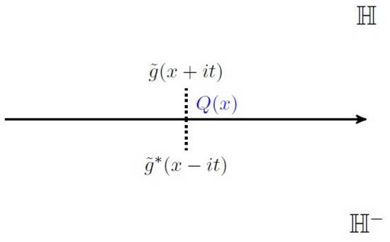
Figure 6. A pair of quantum modular forms, false and mock theta functions [53].

Roughly speaking, it is the holomorphic part of a harmonic Maass forms. The formal definition is given as follows.

Definition  4

([53]). A holomorphic function f on $\mathbb{H}$ is a mock modular form of weight k and multiplier χ, if and only if there exists a weight $2-k$ cusp form g on Γ such that the non-holomorphic completion of f defined by

$$\widehat{f}\left(\tau \right)=f\left(\tau \right)-g^{\ast }\left(\tau \right),\tau \in \mathbb{H}$$

satisfies $\widehat{f}{|}_{k,\chi }\gamma =\widehat{f}$ for every $\gamma \in \Gamma$ and

$$g^{\ast }\left(\tau \right):={\displaystyle \frac{{\left(i2\pi \right)}^{w-1}}{\Gamma (w-1)}}{\int }_{-\overline{\tau }}^{i\infty }{({\tau }^{\prime }+\tau )}^{-k}\overline{g(-{\overline{\tau }}^{\prime })}fd{\tau }^{\prime },$$

$$\widehat{f}{|}_{k,\chi }\gamma =f\left({\displaystyle \frac{a\tau +b}{c\tau +d}}\right)\chi \left(\gamma \right){(c\tau +d)}^{-k},\gamma =\left(\begin{array}{cc}a& b\\ c& d\end{array}\right)$$

Remark  17.

In the above $\Gamma =SL(2,\mathbb{Z})$ or $\Gamma ={\Gamma }_0\left(N\right)$, the congruence subgroup of $SL(2,\mathbb{Z})$.

In the physics context, let us recall that ${\widehat{Z}}_b(-Y)\left(q\right)$ appeared in Section 2.2 and Section 2.5. It is a necessary for testing the superconformal index of $3d\mathcal{N}=2$ SCFTs and the effective central charge. It is clear that orientation reversal is necessary for a complete understanding of ${\widehat{Z}}_b\left(q\right)$ for all types of plumbed manifolds.

Although there are available approaches to find ${\widehat{Z}}_b(-Y)\left(q\right)$, they have limited applicability or difficulty to implement in practice. We summarize the approaches:

• q-Hypergeometric series: It was shown in [53] that ${\widehat{Z}}_b\left(Y\right)\left(q\right)$ of particular Seifert fibered manifolds with three singular fibers, for example, $\Sigma (2,3,5)$ and $\Sigma (2,3,7)$, can be expressed in terms of q-hypergeometric series. It is a rational function, which allows us to apply $q\to 1/q$ to obtain ${\widehat{Z}}_b(-Y)\left(q\right)$ straightforwardly. A caveat of this method is the a q-series can be expressed in multiple ways in terms the q-hypergeometric series; thus, there is non-uniqueness. Each expression leads to a different q-series after $q\to 1/q$, and one of them is the desired ${\widehat{Z}}_b(-Y)\left(q\right)$.
• Rademacher sums: This method is systematic and sophisticated [53]. Obtaining ${\widehat{Z}}_b(-Y)\left(q\right)$ involves finding a certain function in the lower half of the complex plane, which is an image of mock modular form.
• Resurgence method: This method utilizes the quantum modular property of ${\widehat{Z}}_b(Y;q)$ [91] (the resurgence method is a technique that enables one to analyze strongly coupled QFTs. It was applied to the complex Chern–Simons theory in [92]). The method aims to find a dual ${\Psi }_{m,r}{\left(q\right)}^{\vee }$ of a false theta function ${\Psi }_{m,a}\left(q\right)$:

  $${\Psi }_{m,a}\left(q\right)⟷{\Psi }_{m,a}{\left(q\right)}^{\vee }$$
  A starting point for obtaining ${\Psi }_{m,a}{\left(q\right)}^{\vee }$ is the Borel–Mordell integral and its unique decomposition,

  $$J_{(p,a)}(\hslash ):={\displaystyle \frac{1}{-\hslash }}{\int }_0^{\infty }du{e}^{p{u}^2/\hslash }{\displaystyle \frac{sinh\left(\right(p-a\left)u\right)}{sinh\left(pu\right)}},\hslash <0.$$

  (21)

  $$\sqrt{{\displaystyle \frac{4p(-\hslash )}{\pi }}}{J}_{(p,a)}(\hslash )=q^{{\Delta }_a}{F}_a\left(q\right)+i\sqrt{{\displaystyle \frac{\pi }{\hslash }}}\sum _{b=1}^{Floor\left[{\displaystyle \frac{p}{2}}\right]}{S}_{ab}{\tilde{q}}^{{\tilde{\Delta }}_b}{W}_b\left(\tilde{q}\right),q=e^{\hslash },\tilde{q}=e^{{\displaystyle \frac{{\pi }^2}{\hslash }}},$$

  where $F_a\left(q\right)$ is a q-series and $W_b$ is a $\tilde{q}$-series. Using (21) and the numerical analysis, $F_a\left(q\right)$ and $W_b\left(\tilde{q}\right)$ are determined (an analytic continuation of (28) into the $\hslash >0$ regime is given in Section 4.6 of [91]), and they include the desired mock theta functions ${\Psi }_{m,a}{\left(q\right)}^{\vee }$.

Remark 18.

In the above, $p=m$, and $a=r$ from Section 2.3.

4.

Indefinite theta functions: Instead of using the negative definite lattice for the theta function in (4), an application of indefinite lattice theta functions was introduced in [93]. Specifically, it used an indefinite lattice theta function together with a regulator. In this approach, there is a choice of a one-sided cone when summing over lattice vectors. This idea was further pursued and refined in [59], which used a double cone.

An example in which q-hypergeometric series method can be applied is $\Sigma (2,3,7)$ [53]. Using (13), we have

$$\widehat{Z}(\Sigma (2,3,7);q)=q^{83/168}{\Psi }_1^{42+6,14,21}\left(q\right)\left|q\right|<1$$

$${\Psi }_1^{42+6,14,21}\left(q\right)=q^{1/168}\sum _{n=0}^{\infty }{\displaystyle \frac{{(-1)}^n{q}^{\frac{n(n+1)}{2}}}{{(q^{n+1};q)}_n}}$$

We next invert q to jump to the $\left|q\right|>1$ region and use the identity

$${(x;q^{-1})}_n={(-1)}^n{x}^n{q}^{-{\displaystyle \frac{n(n-1)}{2}}}{(a^{-1};q)}_n.$$

Then we arrive at

$${\Psi }_1^{42+6,14,21}\left(q^{-1}\right)=q^{-1/168}\sum _{n=0}^{\infty }{\displaystyle \frac{q^{n^2}}{{(q^{n+1};q)}_n}}=q^{-1/168}{F}_0\left(q\right)$$

$$\widehat{Z}(-\Sigma (2,3,7);q)=q^{-1/2}\left(1+q+q^3+q^4+q^5+2q^7+q^8+2q^9+q^{10}+2q^{11}+q^{12}+\cdots \right)$$

Compared with the result in Section 2.2, the coefficients are no longer $\pm 1$.

3. Series Invariant for Link Complements

3.1. A Two-Variable Series for Knots

Motivated by (4), a multi-variable series for complements of plumbed knots was defined in [51]. We begin by reviewing plumbed knots.

Plumbed knot complements, more generally plumbed 3-manifolds with a torus boundary, are represented by a weighted graph ${\Gamma }_K$ with one distinguished vertex $v_{\ast }$ [51]. This vertex represent the torus boundary. We are interested in the case when the degree of $v_{\ast }$ is one. From the viewpoint of the surgery link $L\left({\Gamma }_K\right)$ described above, an unknot corresponding to $v_{\ast }$ acts as a spectator during the surgery operation. Furthermore, removing $v_{\ast }$ and the edge connecting it to ${\Gamma }_K$ represents an ambient plumbed 3-manifold $Y\left(\widehat{\Gamma }\right)$.

An additional data describing a knot is a framing that takes values in $\mathbb{Z}$. Roughly speaking, this value characterizes the twisting of a longitude of the knot around the knot. This information is captured by weight $k_{v_{\ast }}$ of $v_{\ast }$. This is called graph framing. Therefore, complement of a plumbed knot in $Y\left(\widehat{\Gamma }\right)$ is specified by $({\Gamma }_K,v_{\ast })$. A simple example is shown in Figure 7. The Neumann moves in Figure 1 also apply to plumbing graphs of knots, except the blow-up/-down move on $v_{\ast }$.

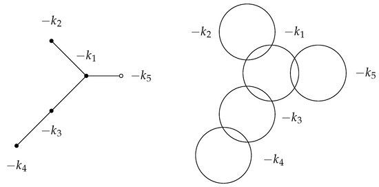
Figure 7. A plumbing graph ${\Gamma }_K$ of a knot $K\subset S^3$ (left) and corresponding surgery link $L\left({\Gamma }_K\right)$ (right). The linking between two link components is the Hopf link. This link diagram can be transformed into a knot diagram through the Kirby moves.

We review the method for obtaining plumbing graphs of torus knots in [51]. We consider torus knots $T(s,t)\subset S^3$, where $gcd(s,t)=1,2\le s<t$. Torus knots are examples of algebraic knots. Hence, they and more precisely their complements admit plumbing graph presentations. The graphs consist of one multivalency vertex having degree 3, weight $-1$, and three legs attached to the vertex. One of the legs has an open vertex of degree 1 called distinguished vertex, representing a torus boundary of the knot complement. To find vertices and weights on the other legs, we solve

$${\displaystyle \frac{t^{\prime }}{t}}+{\displaystyle \frac{s^{\prime }}{s}}=1-{\displaystyle \frac{1}{st}}$$

for unique integers $t^{\prime }\in (0,t)$ and $s^{\prime }\in (0,s)$ satisfying

$$s{t}^{\prime }\equiv -1\left(\mathrm{mod}t\right)t{s}^{\prime }\equiv -1\left(\mathrm{mod}s\right).$$

Then we expand $-t/t^{\prime }$ and $-s/s^{\prime }$ in continued fractions in Section 3.1. Each of them forms a leg with weights attached to the central vertex. The weight of the distinguished vertex is given by $-st$ (this value corresponds to 0-framed torus knots). Example of plumbing graphs are shown in Figure 8.

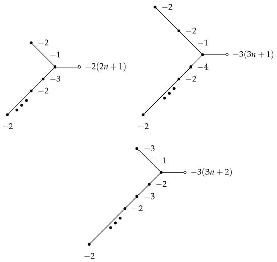
Figure 8. Plumbing graphs of $T(2,2n+1)$ (left), $T(3,3n+1)$ (right), and $T(3,3n+2)$ (bottom). The ellipsis indicates intermediate vertices with weight $-2$ along the legs. The total number of $-2$ vertices in succession on the leg is $n-1$ for $T(2,2n+1),T(3,3n+1)$, and $T(3,3n+2)$.

For complements of plumbed knots that are (weakly) negative definite $({\Gamma }_K,v_{\ast })$, a three-variable series was defined [51]:

$$\begin{array}{c}\hfill \begin{array}{cc}\hfill {\widehat{Z}}_b({\Gamma }_K;z,n,q)& ={(-1)}^{\pi }{\left(z-{\displaystyle \frac{1}{z}}\right)}^{1-\mathrm{deg}\left(v_{\ast }\right)}{q}^{{\displaystyle \frac{3\sigma -TrB}{4}}}\prod _{\begin{array}{c}v\in Vert\\ v\ne v_{\ast }\end{array}}{\oint }_{|z_v|=1}{\displaystyle \frac{d{z}_v}{i2\pi z_v}}{\left(z_v-{\displaystyle \frac{1}{z_v}}\right)}^{2-\mathrm{deg}\left(v\right)}{\Theta }_b^{-Y_K}(\overrightarrow{z},q),\hfill \\ \hfill {\Theta }_b^{-Y_K}& =\sum _{\overrightarrow{l}}{q}^{-{\displaystyle \frac{(\overrightarrow{l},B^{-1}\overrightarrow{l})}{4}}}\prod _{v\in Vert}{z}_v^{l_v},\hfill \end{array}\end{array}$$

(22)

where $Vert$ denotes a set of vertices of ${\Gamma }_K$ and B is the linking matrix of $L\left({\Gamma }_K\right)$. We note that there is no integration over $v_{\ast }$ in (22).

Using the properties of the plumbed knot complements, it was shown that (22) reduces to an independent two-variable series denoted by $F_K(x,q)$. It turns out that $F_K(x,q)$ has the following general form for all knots in $\mathbb{Z}H{S}^3$:

$$F_K(x,q)=\sum _{\begin{array}{c}m=1\\ \mathrm{odd}\end{array}}^{\infty }{f}_m(K;q)\left(x^{m/2}-x^{-m/2}\right)\in {\displaystyle \frac{1}{2^c}}{q}^{\Delta }\mathbb{Z}[q^{-1},q]]\left[[x^{1/2},x^{-1/2}]\right]$$

(23)

where $c\in {\mathbb{Z}}_{\ge 0},\Delta \in \mathbb{Q}$ and $x=z^2$.

Remark  19.

The variable x in (23) counts with the relative $Spi{n}^c$ structures of the knot complement.

Remark  20.

Generally, the coefficient functions $\left\{f_m(K;q)\right\}$ are a Laurent power series $\mathbb{Z}[q^{-1},q]]$; knots whose Alexander polynomials are non-monic have this property. In case of fibered knots, they are Laurent polynomials.

3.2. Large Color R-Matrix

Inspired by the quantum R-matrix formulation of the colored Jones polynomials, R-matrix formulation for $F_K(x,q)$ was constructed in [58]. This approach revealed the infinite-dimensional Verma module structure of quantum group $U_q\left(sl\left(2\right)\right)$ at generic q underlying $F_K(x,q)$. From a computational viewpoint, the R-matrix formulation vastly extended the classes of knots for which $F_K$ can be computed. For example, positive braid knots and positive double-twist knots were computed explicitly in [58]; both of them are infinite families of knots. As in the case of colored Jones polynomials, the R-matrix approach utilizes a braid presentation $\beta$ of K in Figure 9, and the R-matrix acts on the infinite-dimensional Verma modules of $U_q\left(sl\left(2\right)\right)$ over $\mathcal{F}:=\mathbb{C}(x^{1/2},q^{1/2})$. There are two such modules. One of them is the highest-weight Verma module $V_{\infty ,\lambda }^h$ with the highest- weight $\lambda$:

$$\cdots \rightleftharpoons V_{\infty }^h(\lambda -2)\rightleftharpoons V_{\infty }^h\left(\lambda \right),$$

where the top and the bottom maps are e and f generators of $U_q\left(sl\left(2\right)\right)$, respectively. There is a basis ${\left\{v^j\right\}}_{j\ge 0}$ with $v^j\in V_{\infty }^h(\lambda -2j)$ for which the actions of $U_q\left(sl\left(2\right)\right)$ are given by

$$\begin{array}{cc}\hfill e{v}^j& =\left[j\right]v^{j-1}\hfill \\ \hfill f{v}^j& =[\lambda -j]v^{j+1}\hfill \\ \hfill q^{{\displaystyle \frac{h}{2}}}{v}^j& =q^{{\displaystyle \frac{\lambda -2j}{2}}}{v}^j,\hfill \end{array}$$

where $\left[k\right]:={\displaystyle \frac{q^{k/2}-q^{-k/2}}{q^{1/2}-q^{-1/2}}}$. The second one is the lowest-weight Verma module$V_{\infty ,\lambda }^l$ with lowest-weight $\lambda$:

$$V_{\infty }^l\left(\lambda \right)\rightleftharpoons V_{\infty }^l(\lambda +2)\rightleftharpoons \cdots ,$$

where the top and bottom maps are e and f generators, respectively. There is a basis ${\left\{v_j\right\}}_{j\ge 0}$ with $v_j\in V_{\infty }^l(\lambda +2j)$ for which the action of $U_q\left(sl\left(2\right)\right)$ is given by

$$\begin{array}{cc}\hfill e{v}_j& =[-\lambda -j]v_{j+1}\hfill \\ \hfill f{v}_j& =\left[j\right]v_{j-1}\hfill \\ \hfill q^{{\displaystyle \frac{h}{2}}}{v}_j& =q^{{\displaystyle \frac{\lambda +2j}{2}}}{v}_j.\hfill \end{array}$$

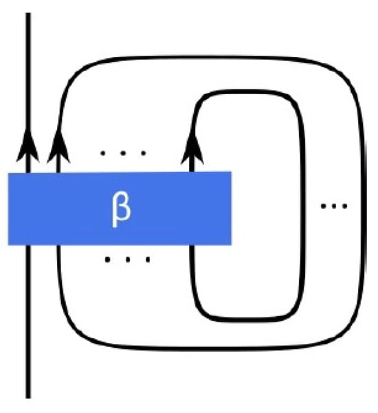
Figure 9. Braid $\beta$, more precisely $(1,1)$-tangle setup.

Remark  21.

The color $n=lo{g}_{q}x$ does not need to be an integer.

Remark  22.

The effects of e and f on the bases are interchanged for highest- and lowest-weight Verma modules.

The quantum R-matrix on the Verma modules for $F_K(x,q)$ for positive and negative crossings (see Figure 10) are given in [58] as

$$\begin{array}{c}\hfill \begin{array}{cc}\hfill \check{R}{\left(x\right)}_{i,j}^{i^{\prime },j^{\prime }}& ={\delta }_{i+j,i^{\prime }+j^{\prime }}{q}^{{\displaystyle \frac{j^{\prime }+j^{\prime }+1}{2}}}{x}^{-{\displaystyle \frac{j^{\prime }+j^{\prime }+1}{2}}}{q}^{j{j}^{\prime }}{\left[\begin{array}{c}i\\ j^{\prime }\end{array}\right]}_q\prod _{1\le l\le i-j^{\prime }}\left(1-q^{j+l}{x}^{-1}\right)\hfill \\ \hfill {\check{R}}^{-1}{\left(x\right)}_{i,j}^{i^{\prime },j^{\prime }}& ={\delta }_{i+j,i^{\prime }+j^{\prime }}{q}^{-{\displaystyle \frac{i+i^{\prime }+1}{2}}}{x}^{{\displaystyle \frac{i+i^{\prime }+1}{2}}}{q}^{-i{i}^{\prime }}{\left[\begin{array}{c}j\\ i^{\prime }\end{array}\right]}_{q^{-1}}\prod _{1\le l\le j-i^{\prime }}\left(1-q^{-i-l}x\right)\hfill \end{array}\end{array}$$

(24)

respectively. These large color R-matrices satisfy the quantum Yang–Baxter equation

$${\check{R}}_{23}{\check{R}}_{12}{\check{R}}_{23}={\check{R}}_{12}{\check{R}}_{23}{\check{R}}_{12}.$$

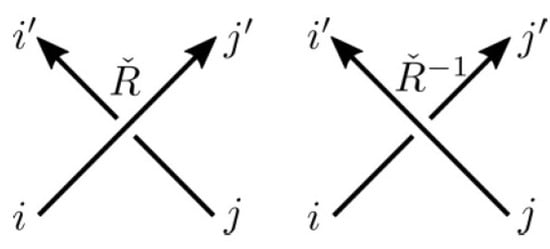
Figure 10. $\check{R}$ and ${\check{R}}^{-1}$ matrices for positive and negative crossings, respectively, are shown.

Compactly, the definition of $F_K$ in terms of a braid closure and hence the R-matrices is given by

$$F_K^{\pm }(x,q)=(x^{1/2}-x^{-1/2})T{r}_q^{\prime }{\beta }_{V_{\infty }^{h,l}},$$

(25)

where the superscript ± denotes positive or negative x-expansions of (27) and $T{r}_q^{\prime }$ is the reduced quantum trace (Reduced refers to opening up a braid as in Figure 9. It is related to the usual quantum trace (see Section 4 of [58] for details)).

Remark  23.

An important aspect of the state sum formulation ($F_K=$ Tr) is (absolute) convergence of power series in $x^{\pm 1}$ and q. This restricts to classes of knots in which (25) is applicable. For example, positive braid knots, fibered strongly quasi-positive braid knots, and positive double-twist knots have been computed.

For the above classes of knots ${\beta }_K$, we have

$$F_K^{-}(x,q)=(x^{1/2}-x^{-1/2})T{r}_q^{\prime }{\beta }_{V_{\infty }^h}.$$

In case of mirror knot of ${\beta }_K$, $V^h$ is replaced by $V^l$ and $F^{-}$ becomes $F^{+}$. The other half can be obtained using Weyl symmetry.

Remark  24.

If two crossing strands are colored by different representations, (24) become functions of x and y variables (see Section 3.2 in [58] for details).

The above large color R-matrix was generalized to representations of $U_q\left(sl\left(N\right)\right)$ in [57]. In the higher-rank case, infinite Verma modules form high-dimensional lattice, whose dimension depends on the value of N. For example, when $N=3$, the dimension of the lattice is two. This is because $U_q\left(sl\left(3\right)\right)$-Verma modules are labeled by $V_{i,j},i,j\ge 0$. Examples of positive braid knots and homogeneous braid knots have been computed in [57].

We move onto the link generalization $F_L$ of $F_K(x,q)$.

3.3. Inverted State Sums

A generalization of (23) to links was achieved in [59]. The main features of the generalizations are domain extensions of (24) and (25) and the introduction of four building blocks of braids, as shown in Figure 11. Specifically, the domains of $i,j,i^{\prime },$ and $j^{\prime }$ are extended to the set of all integers. In the case where two strands of a braid are the same, the R-matrices are given by

$$\check{R}{\left(x\right)}_{i,j}^{i^{\prime },j^{\prime }}=\left\{\begin{array}{cc}{\delta }_{i+j,i^{\prime }+j^{\prime }}{q}^{{\displaystyle \frac{j^{\prime }+j^{\prime }+1}{2}}}{x}^{-{\displaystyle \frac{j^{\prime }+j^{\prime }+1}{2}}}{q}^{j{j}^{\prime }}{\left[\begin{array}{c}i\\ i-j^{\prime }\end{array}\right]}_q\prod _{1\le l\le i-j^{\prime }}\left(1-q^{j+l}{x}^{-1}\right),\hfill & i\ge j^{\prime }\ge 0or\hfill \\ \phantom{1}\hfill & 0>i\ge j^{\prime }\hfill \\ {\delta }_{i+j,i^{\prime }+j^{\prime }}{q}^{{\displaystyle \frac{j^{\prime }+j^{\prime }+1}{2}}}{x}^{-{\displaystyle \frac{j^{\prime }+j^{\prime }+1}{2}}}{q}^{j{j}^{\prime }}{\left[\begin{array}{c}i\\ j^{\prime }\end{array}\right]}_q{\displaystyle \frac{1}{{\prod }_{0\le l\le j^{\prime }-i-1}\left(1-q^{j-l}{x}^{-1}\right)}},\hfill & j^{\prime }\ge 0>i\hfill \\ 0\hfill & otherwise\hfill \end{array}\right.$$

(26)

$${\check{R}}^{-1}{\left(x\right)}_{i,j}^{i^{\prime },j^{\prime }}=\left\{\begin{array}{cc}{\delta }_{i+j,i^{\prime }+j^{\prime }}{q}^{-{\displaystyle \frac{i+i^{\prime }+1}{2}}}{x}^{{\displaystyle \frac{i+i^{\prime }+1}{2}}}{q}^{-i{i}^{\prime }}{\left[\begin{array}{c}j\\ j-i^{\prime }\end{array}\right]}_{q^{-1}}\prod _{1\le l\le j-i^{\prime }}\left(1-q^{-i-l}x\right),\hfill & j\ge i^{\prime }\ge 0or\hfill \\ \phantom{1}\hfill & 0>j\ge i^{\prime }\hfill \\ {\delta }_{i+j,i^{\prime }+j^{\prime }}{q}^{-{\displaystyle \frac{i+i^{\prime }+1}{2}}}{x}^{{\displaystyle \frac{i+i^{\prime }+1}{2}}}{q}^{-i{i}^{\prime }}{\left[\begin{array}{c}j\\ i^{\prime }\end{array}\right]}_{q^{-1}}{\displaystyle \frac{1}{{\prod }_{1\le l\le i^{\prime }-j-1}\left(1-q^{-i+l}x\right)}},\hfill & i^{\prime }\ge 0>j\hfill \\ 0\hfill & otherwise\hfill \end{array}\right.$$

(27)

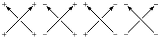
Figure 11. Crossing for the inverted state sum.

In the case where two strands of a braid are different, we need multicolored R-matrices. The strand associated with $i\to j^{\prime }$ is assigned an x variable, whereas the strand associated with $j\to i^{\prime }$ is assigned a y variable. The extended multicolored R-matrices are given by

$$\check{R}{(x,y)}_{i,j}^{i^{\prime },j^{\prime }}=\left\{\begin{array}{cc}{\delta }_{i+j,i^{\prime }+j^{\prime }}{q}^{{\displaystyle \frac{j^{\prime }+j^{\prime }+\frac{1}{2}}{2}}}{x}^{-{\displaystyle \frac{i^{\prime }+j^{\prime }+1}{4}}}{y}^{-{\displaystyle \frac{3j^{\prime }-i^{\prime }+1}{4}}}{q}^{j{j}^{\prime }}{\left[\begin{array}{c}i\\ i-j^{\prime }\end{array}\right]}_q\prod _{1\le l\le i-j^{\prime }}\left(1-q^{j+l}{y}^{-1}\right),\hfill & i\ge j^{\prime }\ge 0or\hfill \\ \phantom{1}\hfill & 0>i\ge j^{\prime }\hfill \\ {\delta }_{i+j,i^{\prime }+j^{\prime }}{q}^{{\displaystyle \frac{j^{\prime }+j^{\prime }+\frac{1}{2}}{2}}}{x}^{-{\displaystyle \frac{i^{\prime }+j^{\prime }+1}{4}}}{y}^{-{\displaystyle \frac{3j^{\prime }-i+1}{4}}}{q}^{j{j}^{\prime }}{\left[\begin{array}{c}i\\ j^{\prime }\end{array}\right]}_q{\displaystyle \frac{1}{{\prod }_{0\le l\le j^{\prime }-i-1}\left(1-q^{j-l}{y}^{-1}\right)}},\hfill & j^{\prime }\ge 0>i\hfill \\ 0\hfill & otherwise\hfill \end{array}\right.$$

(28)

$${\check{R}}^{-1}{(x,y)}_{i,j}^{i^{\prime },j^{\prime }}=\left\{\begin{array}{cc}{\delta }_{i+j,i^{\prime }+j^{\prime }}{q}^{-{\displaystyle \frac{i+i^{\prime }+\frac{1}{2}}{2}}}{x}^{{\displaystyle \frac{3i^{\prime }-j+1}{4}}}{y}^{{\displaystyle \frac{j^{\prime }+i+1}{4}}}{q}^{-i{i}^{\prime }}{\left[\begin{array}{c}j\\ j-i^{\prime }\end{array}\right]}_{q^{-1}}\prod _{1\le l\le j-i^{\prime }}\left(1-q^{-i-l}x\right),\hfill & j\ge i^{\prime }\ge 0or\hfill \\ \phantom{1}\hfill & 0>j\ge i^{\prime }\hfill \\ {\delta }_{i+j,i^{\prime }+j^{\prime }}{q}^{-{\displaystyle \frac{i+i^{\prime }+\frac{1}{2}}{2}}}{x}^{{\displaystyle \frac{3i^{\prime }-j+1}{2}}}{y}^{{\displaystyle \frac{j^{\prime }+i+1}{4}}}{q}^{-i{i}^{\prime }}{\left[\begin{array}{c}j\\ i^{\prime }\end{array}\right]}_{q^{-1}}{\displaystyle \frac{1}{{\prod }_{1\le l\le i^{\prime }-j-1}\left(1-q^{-i+l}x\right)}},\hfill & i^{\prime }\ge 0>j\hfill \\ 0\hfill & otherwise\hfill \end{array}\right.$$

(29)

Over- and under-crossings carry signs, which result in four kinds of crossings, as shown in Figure 11. The signs are tied to the highest- and lowest-weight Verma modules. There are rules for assigning signs to crossings in a braid diagram, more precisely (1,1)-tangle (see Section 1.3 of [59] for details).

Remark  25.

The two-variable extended R-matrices in (28) and (29) can be obtained from the two-variable R-matrices in Section 3.2 of [58].

Using these building blocks, $F_L$ for any homogenous links (the definition of homogenous links is that each generator ${\sigma }_k$ of their braid group appears with either positive or negative powers in a braid word) can be computed. We state the definition of the inverted state sum.

Definition  5

([59]). Given a homogeneous braid diagram β, the inverted state sum is

$$Z^{inv}\left(\beta \right):={(-1)}^s\sum \left(R\cdots R\right),$$

where

$$s=♯\left(\mathrm{columns}\mathrm{with}\mathrm{negative}\mathrm{crossings}\right)+♯\left({\check{R}}^{-1}\right).$$

Theorem  4

([59]). For any homogeneous braid link L with a homogeneous braid diagram ${\beta }_L$, let

$$F_L:=(x^{1/2}-x^{-1/2})Z^{inv}\left({\beta }_L\right),$$

where x is the parameter associated to the open strand. Then $F_L$ is an invariant of L. That is, it is independent of the choice of the homogeneous braid representative.

The above series $F_L$ is a function of $x_1,\cdots ,x_l,q$, where l is the number of components of L.

Remark  26.

There are more statements in the above theorem. They are written in Section 3.7.

3.4. Inverted Cyclotomic Series

Among several representations of the colored Jones polynomials $J_n(K;q)$ of a knot K, there is a particular expression that separates topological and algebraic information of the polynomials and takes values in a completion of the Laurent polynomial ring over the integers [94]. This is often called cyclotomic expansion of the colored Jones polynomials (the cyclotomic expansion is also valid for links). Specifically, for a knot colored by n-dimensional irreducible representation $V_n$ of $sl\left(2\right)$, its cyclotomic expansion of $J_n(K;q)$ is given by (this formula is for 0-framed K)

$$\begin{array}{c}\hfill \begin{array}{cc}\hfill J_n(K;q)& =\sum _{m=0}^{\infty }{a}_m(K;q){\sigma }_m(q^n,q)\hfill \\ \hfill {\sigma }_m(q^n,q)& =\prod _{j=1}^m\left(q^n+q^{-n}-q^j-q^{-j}\right)\in Z\left(U_{\hslash }\right),\hfill \end{array}\end{array}$$

(30)

where $a_m\left(K\right)\in \mathbb{Z}\left[q^{\pm 1}\right]\subset \mathbb{Q}\left[[\hslash ]\right]$ and $q=e^{\hslash }$. The knot information is completely captured by $a_m(K;q)$, and ${\sigma }_m$ are basis elements of $Z\left(U_{\hslash }\right)$. The cyclotomic expansion manifests the integrality property of $J_n(K;q)$. Some examples of $a_m(K;q)$ are

$$a_m\left(3_1^l\right)={(-1)}^m{q}^{{\displaystyle \frac{m(m+3)}{2}}},a_m\left(3_1^r\right)={(-1)}^m{q}^{-{\displaystyle \frac{m(m+3)}{2}}},a_m\left(4_1\right)=1.$$

(31)

Motivated by (30), an inverted cyclotomic expansion for $F_K(x,q)$ was introduced in [59]. Two modifications are as follows: the domain of m of $a_m(K;q)$ was extended to the set of all integers, and ${\sigma }_m$ was inverted. Specifically, we have the following conjectural formula.

Conjecture  6

([59]). For any knot K with ${\Delta }_K\left(x\right)\ne 1$, it has an inverted Habiro series, and it agrees with the $F_K$ in the sense that

$$F_K(x,q)=-(x^{1/2}-x^{-1/2})\sum _{m=1}^{\infty }{\displaystyle \frac{a_{-m}(K;q)}{{\prod }_{j=0}^{m-1}\left(x+x^{-1}-q^j-q^{-j}\right)}}$$

(32)

where the right-hand side is expanded into a power series in x.

The extensions of (31) are

$$a_{-m}\left(3_1^l\right)={(-1)}^m{q}^{{\displaystyle \frac{m(m-3)}{2}}},a_{-m}\left(3_1^r\right)={(-1)}^m{q}^{-{\displaystyle \frac{m(m-3)}{2}}},a_{-m}\left(4_1\right)=1.$$

Remark  27.

In case of links, inverted ${\sigma }_m(x_i,q)$ for each i-th link component $L_i$ appears in the denominator of (32).

The two expressions of $F_K(x,q)$, namely, (23) and (32) are related as follows.

Proposition  4

([59]). If we write

$$-(x^{1/2}-x^{-1/2})\sum _{m=1}^{\infty }{\displaystyle \frac{a_{-m}(K;q)}{{\prod }_{j=0}^{m-1}\left(x+x^{-1}-q^j-q^{-j}\right)}}=x^{1/2}\sum _{j=0}^{\infty }{f}_j(K;q)x^j,$$

then

$$\begin{array}{cc}\hfill f_j(K;q)& =\sum _{i=0}^j\left[\begin{array}{c}j+i\\ 2i\end{array}\right]a_{-i-1}(K;q),\hfill \\ \hfill a_{-i-1}(K;q)& =\sum _{i=0}^j{(-1)}^{i+j}\left[\begin{array}{c}2i\\ i-j\end{array}\right]{\displaystyle \frac{[2j+1]}{[i+j+1]}}{f}_j(K;q).\hfill \end{array}$$

We will see in the next section that (39) is useful for predicting a surgery formula for positive integer slopes.

Remark  28.

An analysis of residues of $F_K(x,q)$ was investigated in [95].

3.5. Dehn Surgery Formulas

Surgery is an indispensable tool in topology. It consists of cutting and gluing manifolds. It provides different perspectives on manifolds and relates them appropriately, thereby revealing multiple presentations of a manifold. This in turn allows for the analysis of manifolds having sophisticated topology. In three dimensions, Dehn surgery plays an important role. We first review Dehn surgery.

Let $Y=S^3$ be a closed oriented manifold and K be a knot in Y. We carve out a tubular neighborhood of K, which is diffeomorphic to $S^1\times D^2$. This yields a compact oriented manifold $Y_K$ with a torus boundary. Then we glue a solid torus $S^1\times D^2$ into $Y_K$ along a slope $p/r\in \mathbb{Q}\cup \left\{\infty \right\}$ via a diffeomorphism. When gluing, a meridian of the solid torus is mapped to $p\mu +r\lambda$ on $\partial Y_K=T^2$, where $\mu$ is a meridian and $\lambda$ is a longitude of $T^2$. This results in a closed oriented manifold $Y_{p/r}$.

$$Y_{p/r}=Y_K{\cup }_{T^2}{S}^1\times D^2.$$

Remark  29.

In the case of links in Y, the above operation is be applied to each component $L_i$ of links with its surgery slope $p_i/r_i$.

There is a classical result regarding closed oriented 3-manifolds and Dehn surgery.

Theorem  5

([96,97]). Any closed connected oriented 3-manifold can be obtained from Dehn surgery on (framed) links in $S^3$.

In our setting, Dehn surgery establishes a relation between $F_K$ and $\widehat{Z}$. There are multiple (conjectured) surgery formulas covering different regimes of surgery slopes for a knot. The surgery formulas allow one to access $\widehat{Z}$ of closed oriented 3-manifolds that are beyond plumbed manifolds.

Theorem  6

([51] Plumbed knot surgery). Let Y be the complement of a knot K in $\widehat{Y}=\mathbb{Z}H{S}^3$, and let $Y_{p/r}$ be the result of Dehn surgery along K with coefficient $p/r\in {\mathbb{Q}}^{\ast }$. Suppose that both $\widehat{Y}$ and $Y_{p/r}$ are negative definite plumbed 3-manifolds. Then the surgery on K yields

$${\widehat{Z}}_b(Y_{p/r};q)=ϵq^d{\mathcal{L}}_{p/r}^{\left(b\right)}\left[\left(x^{{\displaystyle \frac{1}{2r}}}-x^{-{\displaystyle \frac{1}{2r}}}\right)F_K(x,q)\right]$$

(33)

where

$${\mathcal{L}}_{p/r}^{\left(b\right)}:x^u{q}^v\mapsto \left\{\begin{array}{cc}{q}^{-u^{2}r/p}{q}^v,\hfill & \mathit{if}ru-b\in p\mathbb{Z}\hfill \\ 0,\hfill & \mathit{otherwise}.\hfill \end{array}\right.$$

for some $ϵ\in \left\{\pm 1\right\}$ and $d\in \mathbb{Q}$.

The above result was conjectured for all knots.

Conjecture  7

([51]). Let $K\in S^3$ be a knot, and let $S_{p/r}^3\left(K\right)$ be the result of Dehn surgery along K with coefficient $p/r\in {\mathbb{Q}}^{\ast }$. Then there exist $ϵ\in \left\{\pm 1\right\}$ and $d\in \mathbb{Q}$ such that

$${\widehat{Z}}_b(S_{p/r}^3\left(K\right);q)=ϵq^d{\mathcal{L}}_{p/r}^{\left(b\right)}\left[\left(x^{{\displaystyle \frac{1}{2r}}}-x^{-{\displaystyle \frac{1}{2r}}}\right)F_K(x,q)\right]$$

(34)

Provided that the right-hand side of this equation is well defined.

The well-defined condition is tied to the sign of the surgery slope $p/r$ and the behavior of $f_m(K;q)$ in (23). In the case when the right-hand side of (34) yields an ill-defined result due to the positivity of the slope $p/r>0$, an idea of regularization was proposed to obtain a convergent q-series in the complex unit disc [59]. Specifically, the regularized surgery formulas for positive surgery slopes $+1/r$ and $+p$ are the following.

Conjecture  8

([59] Regularized $+{\displaystyle \frac{1}{r}}$ surgery). When $+{\displaystyle \frac{1}{r}}$ surgery formula (41) converges, we need to use (41). When it does not converge, we can regularize it in the following way, as long as the regularization converges:

$${\widehat{Z}}_b(S_{+{\displaystyle \frac{1}{r}}}^3\left(K\right);q)=q^{{\displaystyle \frac{r+r^{-1}}{4}}}\sum _{j=0}^{\infty }{f}_j(K;q)\left(q^{-r{(j+{\displaystyle \frac{1}{2}}-{\displaystyle \frac{1}{2r}})}^2}-q^{-r{(j+{\displaystyle \frac{1}{2}}+{\displaystyle \frac{1}{2r}})}^2}\right)\left(1-{\displaystyle \frac{{\sum }_{\left|k\right|\le j}{(-1)}^k{q}^{\frac{k\left(\right(2r+1)k+1)}{2}}}{f(-q^r,-q^{r+1})}}\right)$$

where

$$f(a,b):=\sum _{n\in \mathbb{Z}}{a}^{{\displaystyle \frac{n(n+1)}{2}}}{b}^{{\displaystyle \frac{n(n-1)}{2}}}={(-a;ab)}_{\infty }{(-b;ab)}_{\infty }{(ab;ab)}_{\infty }$$

is the Ramanujan theta function.

The term in the second parenthesis is the regulator.

Conjecture  9

([59] Regularized $+p$ surgery). When $+p$ surgery formula (41) converges, we need to use (41). When it does not converge, we can regularize it in the following way:

$${\widehat{Z}}_b(S_{+p}^3\left(K\right);q)=q^{{\displaystyle \frac{1}{2}}}\sum _{n=0}^{\infty }{a}_{-n-1}\left(K\right){\displaystyle \frac{{(-1)}^n{q}^{\frac{n(n+1)}{2}}}{{(q^{n+1};q)}_n}}{q}^{{\displaystyle \frac{b(p-b)}{p}}}{P}_n^{p,b}\left(q^{-1}\right)$$

provided that the regularization converges. The polynomials $P_n^{p,b}\left(q\right)\in {\mathbb{Z}}_{\ge 0}\left[q^{-1}\right]$.

The above polynomials $P_n^{p,b}\left(q\right)\in {\mathbb{Z}}_{\ge 0}\left[q^{-1}\right]$ arise from the following rational function:

$${\displaystyle \frac{1}{{\prod }_{j=1}^n\left(x+x^{-1}-q^j-q^{-j}\right)}}{|}_{x^u\mapsto {\delta }_{b,u\left(modp\right)}{q}^{-{\displaystyle \frac{u^2}{p}}}}={\displaystyle \frac{{(-1)}^n{q}^{\frac{n(n+1)}{2}}}{{(q^{n+1};q)}_n}}{q}^{{\displaystyle \frac{b(p-b)}{p}}}{P}_n^{p,b}\left(q^{-1}\right).$$

A list of $P_n^{p,b}$ is available in [54].

Up to this point, we have been focusing on knot surgeries. In the case of links, a formula for Dehn surgery on links along integer surgery slopes has been conjectured.

Conjecture  10

([58] Integral link surgery). Let $S_{p_1,\cdots ,p_l}^3\left(L\right)$ be the 3-manifold obtained by $(p_1,\cdots ,p_l)$ surgery on $L\subset S^3$, and let B be the $l\times l$ linking matrix defined by

$$B=\left\{\begin{array}{c}{p}_i,\mathit{if}i=j,\hfill \\ lk(i,j),\mathit{otherwise}\hfill \end{array}\right.$$

Let

$${\mathcal{L}}_B^b:x^u\mapsto \left\{\begin{array}{c}{q}^{-(u,B^{-1}u)},\mathit{if}u\in b+B{\mathbb{Z}}^l\hfill \\ 0,\mathit{otherwise}\hfill \end{array}\right.$$

Then

$${\widehat{Z}}_b\left(S_{p_1,\cdots ,p_l}^3\left(L\right)\right)=ϵq^d{\mathcal{L}}_B^b\left[\left(x_1^{{\displaystyle \frac{1}{2}}}-x_1^{-{\displaystyle \frac{1}{2}}}\right)\cdots \left(x_l^{{\displaystyle \frac{1}{2}}}-x_l^{-{\displaystyle \frac{1}{2}}}\right)F_L(x_1,\cdots ,x_l,q)\right]$$

for some sign $ϵ\in \left\{\pm 1\right\}$ and $d\in \mathbb{Q}$, whenever the right-hand side makes sense.

Remark  30.

A surgery formula for the infinite surgery slope was found in [98].

The above Dehn surgery formulas were generalized in the case of the presence of the line operators in Section 2.4.

Definition  6

([54]). Consider the series $F_K(x,q)$ associated to the plumbed knot K with a defect operator along K in the highest-weight representation of $sl\left(2\right)$ with the highest-weight $\nu \overrightarrow{\omega }$. We define the corresponding defect invariant for the closed manifold $S_{p/r}\left(K\right)$ as

$${\widehat{Z}}_b(S_{p/r}\left(K\right);W_{\nu };q)=ϵq^d{\mathcal{L}}_{p/r}^{b+\nu }\left[(x^{1/2}-x^{-1/2})F_K(x,q){\chi }_{\nu }\left(x^{{\displaystyle \frac{1}{2r}}}\right)\right]$$

where the sl(2) character ${\chi }_{\nu }$ is the same as in (15) and $ϵ,d$ are the same as in (34).

3.6. Perturbative Expansion

A perturbation series in physics reflects the contributions of quantum effects in the spirit of quantum mechanics—that is, how quantum perturbations affect an original system. In the case of quantum invariants of knots, the same idea can be applied. For instance, a connection between colored Jones polynomials $J_n(K;q)$ and Alexander polynomials $\Delta (K;x)$ of a knot K (the knot is 0-framed) was discovered in [99,100,101] and proven in [102]. This relation appears in the perturbative expansion of the former.

$$\begin{array}{cc}\hfill J_n(K;e^{\hslash })& ={\displaystyle \frac{1}{\Delta \left(x\right)}}+\sum _{r=1}^{\infty }{\displaystyle \frac{P_r\left(x\right)}{\Delta {\left(x\right)}^{2r+1}}}{\hslash }^r\hfill \\ \hfill & =\sum _{m=0}^{\infty }\sum _{j=0}^m{c}_{m,j}{n}^j{\hslash }^m\hfill \end{array}$$

where $P_r\left(x\right)$ are Laurent polynomials. This expansion is natural from viewpoint of the Chern–Simons (CS) gauge theory. It is a weak coupling (i.e., large-CS-level $k\in \mathbb{Z}$) regime of the theory. Motivated by the above perturbative expansion, a similar property was conjectured for $F_K$.

Conjecture  11

([51]). For a knot $K\subset$$S^3$, the asymptotic expansion of the knot invariant $F_K\left(x,q={\mathrm{e}}^{\hslash }\right)$ about $\hslash =0$ coincides with the Melvin–Morton–Rozansky (MMR) expansion of the colored Jones polynomial in the large color limit:

$$\begin{array}{c}{\displaystyle \frac{F_K\left(x,q={\mathrm{e}}^{\hslash }\right)}{x^{1/2}-x^{-1/2}}}=\sum _{r=0}^{\infty }{\displaystyle \frac{P_r\left(x\right)}{{\Delta }_K{\left(x\right)}^{2r+1}}}{\hslash }^r,\end{array}$$

(35)

where $x=e^{n\hslash }$ is fixed, n is the color of K, $P_r\left(x\right)\in \mathbb{Q}\left[x^{\pm 1}\right]$, $P_0\left(x\right)=1$, and ${\Delta }_K\left(x\right)$ is the (symmetrized) Alexander polynomial of K.

A generalization of the above conjecture to links was stated and proved.

Conjecture  12

([58]). There are a link invariant $F_L(x_1,\cdots ,x_l,q)$, a series in $x_1,\cdots ,x_l$, and q with integer coefficients, where l is the number of components of link L, such that

$$F_L(x_1,\cdots ,x_l,e^{\hslash })=\sum _{j=0}^{\infty }{\displaystyle \frac{P_j(L;x_1,\cdots ,x_l)}{{\nabla }_L{(x_1,\cdots ,x_l)}^{2j+1}}}{\displaystyle \frac{{\hslash }^j}{j!}}$$

where the right-hand side is the large color expansion of the colored Jones polynomials $J_L(n_1,\cdots ,n_l;q=e^{\hslash })$ expanded around $\hslash =0$ while keeping $x_i=q^{n_i}=e^{n_i\hslash }$ fixed for each $1\le i\le l$ and ${\nabla }_L$ is the Alexander–Conway function of L.

Theorem  7

([59] Theorem 1 (2)). Let L and $F_L$ be as described in Theorem 4. By setting $q=e^{\hslash }$, the ℏ-expansion of $F_L$ agrees with the MMR expansion of the colored Jones polynomials.

The perturbative analysis has been extended to $F_K$ associated with a Lie algebra $sl\left(3\right)$ for positive braid knots colored by any irreducible representations of $U_q\left(sl\left(3\right)\right)$ (only symmetric representations were considered in [57]) at generic q in [103]. The perturbation series takes the following form.

Theorem  8

([103] $F_K$ for $sl\left(3\right)$). Let ${\beta }_K$ be a positive braid knot. Then the reduced quantum trace ${\widetilde{Tr}}_{V_x^1\otimes V_y^1}^q\left({\beta }_K\right)$ converges in $\mathbb{Z}\left[q^{\pm 1}\right]\left[[x^{-1},y^{-1}]\right]$, and

$$F_K^{sl\left(3\right)}(x,y,q)=\sum _{i,j\ge 0}{f}_{i,j}\left(q\right)x^{i+{\displaystyle \frac{1}{2}}}{y}^{i+{\displaystyle \frac{1}{2}}}$$

is a well-defined knot invariant that satisfies

$$F_K^{sl\left(3\right)}(x,y,e^{{\displaystyle \frac{h}{2}}})=\sum _{j=0}^{\infty }{\displaystyle \frac{P_j(K;x,y)}{{\left({\Delta }_K\left(x\right){\Delta }_K\left(y\right){\Delta }_K\left({\left(xy\right)}^{-1}\right)\right)}^{2j+1}}}{\displaystyle \frac{h^j}{j!}}$$

where $P_j(K;x,y)\in \mathbb{Q}[x^{\pm 1},y^{\pm 1}]$ and $P_0=1$.

3.7. Recursion Method

Another well-known property of the colored Jones polynomials of a knot K in $S^3$ is that they are q-holonomic [104,105] (this property is also valid for links as well). Specifically, they satisfy the recursion relation

$${\widehat{A}}_K(\widehat{x},\widehat{y},q)J_n(K;q)=0,$$

where $n\in \mathbb{N}$ is the color of K and ${\widehat{A}}_K$ is called quantum (noncommutative) A-polynomial of K and is a q-difference operator of the form

$${\widehat{A}}_K(\widehat{x},\widehat{y},q)=\sum _{k=0}^d{g}_k(\widehat{x},q){\widehat{y}}^k.$$

The operators $\widehat{x}$ and $\widehat{y}$ act as

$$\begin{array}{cc}\hfill \widehat{x}{J}_n(K;q)& =q^n{J}_n(K;q)\hfill \\ \hfill \widehat{y}{J}_n(K;q)& =J_{n+1}(K;q)\hfill \end{array}$$

The above recursion relation enables to find $J_n$ for any color. It was conjectured that $F_K$ also satisfies a recursion relation given by the same ${\widehat{A}}_K$ [51].

Conjecture  13

([51]). For any knot $K\subset$$S^3$, the normalized series $f_K(x,q)$ satisfies a linear recursion relation generated by the quantum A-polynomial of K ${\widehat{A}}_K(q,\widehat{x},\widehat{y})$:

$${\widehat{A}}_K(q,\widehat{x},\widehat{y})f_K(x,q)=0,$$

(36)

where $f_K:=F_K(x,q)/\left(x^{1/2}-x^{-1/2}\right)$.

The actions of $\widehat{x}$ and $\widehat{y}$ are

$$\widehat{x}{f}_K(x,q)=x{f}_K(x,q)\widehat{y}{f}_K(x,q)=f_K(xq,q).$$

Conjecture  14

([58]). The link series $F_L(x_1,\cdots ,x_l,q)$ defined in Theorem 4 is annihilated by the quantum A-ideal annihilating of the colored Jones polynomials of L.

Theorem  9

([59] Theorem 1 (3)). Conjecture 13 holds.

3.8. ADO Polynomials

We saw that ${\widehat{Z}}_b\left(q\right)$ at roots of unity are related to other topological invariants of 3-manifolds, as described in Section 2.6. Similarly, evidence for a connection between $F_K(x,q)$ at roots of unity and ADO polynomials of K was discovered in [106]. The latter are non-semisimple quantum invariants [15]. The precise form of the relation is given by the following conjecture.

Conjecture  15

([106]). For any knot K in $S^3$,

$$F_K{(x,q)|}_{q={\zeta }_p}=\left(x^{1/2}-x^{-1/2}\right){\displaystyle \frac{{\mathit{ADO}}_p(K;x,{\zeta }_p)}{{\Delta }_K\left(x^p\right)}}{\zeta }_p=e^{i2\pi /p},p\in {\mathbb{Z}}_{+}.$$

This conjecture was verified for some values of p for the right-handed trefoil and the figure eight knots [106]. Further evidence for the conjectures, including formulas for $AD{O}_3$ and an algorithm for $AD{O}_4$ of a family of torus knots, was given in [107]. We record explicit formulas of ${\mathrm{ADO}}_3$ for $T(2,2s+1)$. They are divided into three types depending on their coefficient pattern:

• For $K=T(2,2s+1)=T(2,3),T(2,9),T(2,15),T(2,21),\cdots$

  $$\begin{array}{c}{\mathrm{ADO}}_3\left(x\right)={\zeta }_3{x}^{2s}+{\zeta }_3{x}^{2s-1}+({\zeta }_3-{\zeta }_3^{-1})x^{2s-2}-{\zeta }_3^{-1}{x}^{2s-3}-{\zeta }_3^{-1}{x}^{2s-4}\hfill \\ +{\zeta }_3{x}^{2s-6}+{\zeta }_3{x}^{2s-7}+({\zeta }_3-{\zeta }_3^{-1})x^{2s-8}-{\zeta }_3^{-1}{x}^{2s-9}-{\zeta }_3^{-1}{x}^{2s-10}\\ \hfill +\cdots +({\zeta }_3-{\zeta }_3^{-1})+(x\to 1/x).\end{array}$$
• For $K=T(2,2s+1)=T(2,5),T(2,11),T(2,17),T(2,23),\cdots$

  $$\begin{array}{c}{\mathrm{ADO}}_3\left(x\right)={\zeta }_3^{-1}{x}^{2s}+{\zeta }_3^{-1}{x}^{2s-1}+({\zeta }_3^{-1}-1)x^{2s-2}-x^{2s-3}-x^{2s-4}\hfill \\ +{\zeta }_3^{-1}{x}^{2s-6}+{\zeta }_3^{-1}{x}^{2s-7}+({\zeta }_3^{-1}-1)x^{2s-8}-x^{2s-9}-x^{2s-10}\\ \hfill +\cdots -1+(x\to 1/x).\end{array}$$
• For $K=T(2,2s+1)=T(2,7),T(2,13),T(2,19),T(2,25),\cdots$

  $$\begin{array}{c}{\mathrm{ADO}}_3\left(x\right)=x^{2s}+x^{2s-1}+(1-{\zeta }_3)x^{2s-2}-{\zeta }_3{x}^{2s-3}-{\zeta }_3{x}^{2s-4}\hfill \\ +x^{2s-6}+x^{2s-7}+(1-{\zeta }_3)x^{2s-8}-{\zeta }_3{x}^{2s-9}-{\zeta }_3{x}^{2s-10}\\ \hfill +\cdots +1+(x\to 1/x).\end{array}$$

All the explicit x terms are polynomials, and the power of x decreases by two after one cycle of a coefficient combination. Another advancement was the introduction of a refinement of $F_K(x,q)$ [108]. It was shown that $F_K(x,q)$ admits two parameter deformations through the superpolynomial [109,110]. This led to a generalization of the above conjecture.

Conjecture  16

([108]). For any knot K in $S^3$, there exists a t-deformation of the symmetric ${\mathrm{ADO}}_p$-polynomial of K for $SU\left(N\right)$,

$${\mathit{ADO}}_p^{SU\left(N\right)}[K;x,t]:={\left({\Delta }_K(x^p,-{(-t)}^p)\right)}^{N-1}\underset{q\to e^{i2\pi /p}}{lim}{F}_K(x,q,a=-q^N/t,t),p\in {\mathbb{Z}}_{+}$$

And the $t=-1$ specialization reduces to the original ${\mathit{ADO}}_p[K;x]$ (up to the rescaling of x).

From Conjecture 16, a refined ${\mathrm{ADO}}_3$ polynomial for $T(2,2s+1)$, $s\in {\mathbb{Z}}_{+}$ is

$${\mathrm{ADO}}_3[T(2,2s+1);x,t]={\left(tx\right)}^{2s}+{\displaystyle \frac{{\zeta }_3^{-1}}{t}}{\left(tx\right)}^{2s-1}+\left({\displaystyle \frac{{\zeta }_3}{t^2}}-{\zeta }_3^{-1}\right){\left(tx\right)}^{2s-2}-{\displaystyle \frac{{\zeta }_3}{t}}{\left(tx\right)}^{2s-3}-{\displaystyle \frac{1}{t^2}}{\left(tx\right)}^{2s-4}$$

$$+{\left(tx\right)}^{2s-6}+{\displaystyle \frac{{\zeta }_3^{-1}}{t}}{\left(tx\right)}^{2s-7}+\left({\displaystyle \frac{{\zeta }_3}{t^2}}-{\zeta }_3^{-1}\right){\left(tx\right)}^{2s-8}-{\displaystyle \frac{{\zeta }_3}{t}}{\left(tx\right)}^{2s-9}-{\displaystyle \frac{1}{t^2}}{\left(tx\right)}^{2s-10}+\cdots +O\left({\displaystyle \frac{1}{tx}}\right),$$

where the $O(1/tx)$ terms are determined by the t-deformed Weyl symmetry of the ${\mathrm{ADO}}_p$ invariant,

$${\mathrm{ADO}}_p^{SU\left(2\right)}(1/x,t)={\mathrm{ADO}}_p^{SU\left(2\right)}({\zeta }_p^{-2}{t}^{-2}x,t).$$

The suppressed polynomial terms follow the same power and coefficient patterns of the previous terms. The three formulas for the original ${\mathrm{ADO}}_3[T(2,2s+1);x]$ coalesce into one formula by the t-deformation.

3.9. Knot–Quiver Correspondence

The connection between knots and quivers was discovered through the identification of a certain knot invariant (the LMOV invariant) with a (motivic) Donaldson–Thomas invariant [111,112]. The significance of this relationship is that it established the integrality of the knot invariant. Additionally, it provided a quiver-theoretic perspective on the structure of colored HOMFLY-PT polynomials and superpolynomials. Furthermore, another consequence of this connection was the generalization of knot invariants from symmetric representations to arbitrary representations.

Another interesting connection between the deformed series $F_K(x,a,q)$ (this series is a series analogue of the colored HOMFLYPT polynomial) and quiver theory [111,112] was discovered in [60]. It was described that $F_K$ can be obtained from the so-called motivic generating seriesthat characterizes a quiver. We begin by reviewing the quiver side.

A quiver Q is an oriented graph consisting of a finite set of vertices $Q_0$ and a finite set of arrows between them $Q_1$ (i.e., ($Q_0,Q_1$)). An adjacency matrix C of Q is the $m\times m$ matrix with entries $C_{ij}$ equal to the number of arrows from i and j, where $m=|Q_0|$. If $C^t=C$, then Q is called a symmetric quiver. A quiver representation is an assignment of a finite dimensional $d_i\in \mathit{d}=(d_1,\cdots ,d_m)$, which is complex vector space, to the vertex $i\in Q_0$ and a linear map ${\gamma }_{ij}:{\mathbb{C}}^{d_i}\to {\mathbb{C}}^{d_j}$ to each arrow from vertex i to j. A goal in quiver representation theory is to investigate modulus spaces of quiver representations. In the case of symmetric quivers, information about the modulus space of representation is encoded in motivic generating series defined as

$$P_Q(x,q):=\sum _{d_1,\cdots ,d_m\ge 0}{(-q^{1/2})}^{\mathit{d}.C.\mathit{d}}\prod _{i=1}^m{\displaystyle \frac{x_i^{d_i}}{{(q;q)}_{d_i}}},$$

(37)

where

$${(z;q)}_n=\prod _{k=0}^{n-1}(1-z{q}^k).$$

In [113], it was shown that the knot–quiver correspondence can be generalized to knot complements of torus knots $T(2,2n+1)$. Specifically, this involves data of a symmetric Q, integers $n_i$, and half-integers $a_i,l_i,i\in Q_0$ to a knot complement $M_K=S^3\setminus \nu \left(K\right)$. Then the deformed $F_K$ can be obtain from (37) as

$$F_K(x,a,q)=P_Q(x,q){|}_{x_i=x^{n_i}{a}^{a_i}{q}^{l_i}}=\sum _{\mathit{d}\ge 0}{(-q^{1/2})}^{\mathit{d}.C.\mathit{d}}{\displaystyle \frac{x^{\mathit{n}.\mathit{d}}{a}^{\mathit{a}.\mathit{d}}{q}^{\mathit{l}.\mathit{d}}}{{\left(q\right)}_{\mathit{d}}}}.$$

(38)

where ${\left(q\right)}_s={(q;q)}_s$.

Remark  31.

We note that the deformed $F_K(x,a,q)$ is associated with an abelian branch of A-polynomial of K. For $F_K$ associated with other branches, see Section 3 of [60].

The general quiver form of $F_{T(2,2p+1)}(x,a,q)$ is given by [108]

$$F_{T(2,2p+1)}(x,a,q)=\sum _{d_1,\cdots ,d_{2p+2}\ge 0}{(-q^{1/2})}^{\mathit{d}.C.\mathit{d}}{\displaystyle \frac{x^{\mathit{n}.\mathit{d}}{a}^{\mathit{a}.\mathit{d}}{q}^{\mathit{q}.\mathit{d}-\frac{1}{2}{\sum }_i{C}_{ii}{d}_i}}{{\left(q\right)}_{\mathit{d}}}}$$

$$C=\left(\begin{array}{ccc}{\mathbf{1}}_{2p}-\mathit{D}& -\mathbf{1}& \mathbf{0}\\ -\mathbf{1}& 1& 0\\ \mathbf{0}& 0& 0\end{array}\right)$$

$$\begin{array}{cc}\hfill \mathit{n}& =\left(1,1,3,3,\cdots ,2p-1,2p-1,1,1\right)\hfill \\ \hfill \mathit{a}& =\left(1,0,\cdots ,1,0,0,0\right)\hfill \\ \hfill \mathit{q}& =\left(0,1,\cdots ,0,1,1,1\right)=1-\mathit{a},\hfill \end{array}$$

where $-\mathbf{1},\mathbf{0}$ denote constant vectors of appropriate size, ${\mathbf{1}}_{2p}$ is the identity matrix, and ${\mathit{d}}_{ij}=min(i,j)-1$ for $1\le i,j\le 2p$.

The converse direction, namely, extracting a quiver structure from $F_K(x,a,q)$, was shown in [60]. For example, we start from $F_K(x,a,q)$, the left-handed trefoil, in the following form:

$$F_{3_1}(x,a,q)=\sum _{k\ge 0}{x}^k{q}^k{\displaystyle \frac{{(x;q^{-1})}_k(a{q}^{-1};q)}{{\left(q\right)}_k}}.$$

We next apply the following identity to $(a{q}^{-1};q)$ (it is Lemma 4.5 in [112]):

$$\begin{array}{cc}\hfill {\displaystyle \frac{{\left(x\right)}_{d_1+\cdots +d_k}}{{\left(q\right)}_{d_1}\cdots {\left(q\right)}_{d_k}}}& =\sum _{{\alpha }_1+{\beta }_1=d_1}\cdots \sum _{{\alpha }_k+{\beta }_k=d_k}{\displaystyle \frac{1}{{\left(q\right)}_{{\alpha }_1}\cdots {\left(q\right)}_{{\alpha }_k}{\left(q\right)}_{{\beta }_1}\cdots {\left(q\right)}_{{\beta }_k}}}\times \hfill \\ \hfill & \times {(-x)}^{{\alpha }_1+\cdots +{\alpha }_k}{q}^{{\displaystyle \frac{1}{2}}\left({\alpha }_1^2+\cdots +{\alpha }_k^2\right)}{q}^{-{\displaystyle \frac{1}{2}}\left({\alpha }_1+\cdots +{\alpha }_k\right)}{q}^{{\sum }_{i=1}^{k-1}{\alpha }_{i+1}(d_1+\cdots +d_k)}\hfill \end{array}$$

Then we get

$$F_{3_1}(x,a,q)=\sum _{d_1^{\prime },d_2^{\prime }\ge 0}{(-1)}^{d_1^{\prime }}{x}^{d_1^{\prime }+d_2^{\prime }}{a}^{d_1^{\prime }}{q}^{d_2^{\prime }}{q}^{(d_1^{\prime 2}-d_1^{\prime })/2}{\displaystyle \frac{{(x;q^{-1})}_{d_1^{\prime }+d_2^{\prime }}}{{\left(q\right)}_{d_1^{\prime }}{\left(q\right)}_{d_2^{\prime }}}}$$

(39)

After using the identity

$${(x;q^{-1})}_d={(x{q}^{1-d};q)}_d={\displaystyle \frac{{(x{q}^{1-d};q)}_{\infty }}{{(xq;q)}_{\infty }}}=\sum _{i,j}{(-1)}^i{x}^{i+j}{q}^{(i^2-i)/2}{q}^{i+j}{q}^{-di}{\displaystyle \frac{1}{{\left(q\right)}_i{\left(q\right)}_j}}.$$

(40)

we arrive at a quiver form

$$F_{3_1}(x,a,q)=\sum _{d_1,\cdots ,d_4\ge 0}{(-q^{1/2})}^{{\sum }_{i,j=1}^4{C}_{ij}{d}_i{d}_j}\prod _{i=1}^4{\displaystyle \frac{x_i^{d_i}}{{\left(q\right)}_{d_i}}},$$

$$C=\left(\begin{array}{cccc}0& 0& 0& -1\\ 0& 1& 0& -1\\ 0& 0& 0& 0\\ -1& -1& 0& 1\end{array}\right),\left(\begin{array}{c}{x}_1\\ x_2\\ x_3\\ x_4\end{array}\right)=\left(\begin{array}{c}xq\\ xa{q}^{-1/2}\\ xq\\ x{q}^{1/2}\end{array}\right).$$

(41)

An alternative identity that can be applied to (39) is

$$\begin{array}{c}\hfill \begin{array}{cc}\hfill {\displaystyle \frac{{(x;q^{-1})}_{d_1+\cdots +d_n}}{{\prod }_{i=n}^1{(q;q)}_{d_i}}}& =\sum _{{\alpha }_1+{\beta }_1=d_1}\cdots \sum _{{\alpha }_n+{\beta }_n=d_n}{(-q^{1/2})}^{{\beta }_1^2+\cdots +{\beta }_n^2+2{\sum }_{i=1}^{n-1}{\beta }_{i+1}(d_1+\cdots d_n)}\hfill \\ \hfill & \times {\displaystyle \frac{{\left(x{q}^{1/2-{\sum }_i{\alpha }_i-{\sum }_i{\beta }_i}\right)}^{{\beta }_1+\cdots +{\beta }_n}}{{\left(q\right)}_{{\alpha }_1}{\left(q\right)}_{{\beta }_1}\cdots {\left(q\right)}_{{\alpha }_n}{\left(q\right)}_{{\beta }_n}}}.\hfill \end{array}\end{array}$$

(42)

An application of this identity yields

$$C=\left(\begin{array}{cccc}0& 0& -1& -1\\ 0& 1& 0& 0\\ -1& 0& -1& -1\\ -1& 0& -1& 0\end{array}\right),\left(\begin{array}{c}{x}_1\\ x_2\\ x_3\\ x_4\end{array}\right)=\left(\begin{array}{c}xq\\ xa{q}^{-1/2}\\ x^2{q}^{3/2}\\ x^{2}a\end{array}\right).$$

(43)

Remark  32.

The final forms (41) and (43) are connected by operations on the vertex of quivers (see [114] for details).

A closely related result in [60] is that colored HOMFLYPT polynomials $P_r(K;a,q)$ of knots K colored by symmetric representation $S^r$ in a quiver form (where the subscript r in $P_r$ refers to $S^r$; there is a conjecture regarding expressing the generating function of the colored HOMFLYPT polynomials in a quiver form in [112]) can be used to obtain $F_K(x,a,q)$. This requires a framing K in a particular way. Let Q be a quiver corresponding to K and $\mathit{a}$ and $\mathit{l}$ be the vectors. Suppose that

$$-C_{\min }\le C_{ij}\le C_{max},i,j=1,\cdots ,m,$$

where $C_{\min },C_{max}\ge 0$. Next, permute rows and columns of C such that $C_{11}=C_{\min }$ and $C_{mm}=C_{max}$. We express $P_r(K;a,q)$ in a quiver form as

$$P_r(K;a,q)=\sum _{d_1+\cdots +d_k=r}{(-1)}^{\sum C_{ii}{d}_i}{a}^{\mathit{a}.\mathit{d}}{q}^{\mathit{l}.\mathit{d}}{q}^{{\displaystyle \frac{1}{2}}\mathit{d}.C.\mathit{d}}{\displaystyle \frac{{\left(q\right)}_r}{{\prod }_{i=1}^k{\left(q\right)}_{d_i}}}.$$

(44)

To convert (44) into $F_K(x,a,q)$, we framed K by $C_{\min }$, which amounts to multiplying $P_r$ by $q^{C_{min}(r^2-r)/2}$ and setting $q^r=x$.

$$\begin{array}{c}\hfill \begin{array}{cc}\hfill F_{K^{f=C_{\min }}}(x,a,q)& ={(-1)}^{r{C}_{\min }}{a}^{r{a}_1}{q}^{r{l}_1}\sum _{d_1,\cdots ,d_m}{(-1)}^{{\sum }_{i\ge 2}(C_{ii}+C_{\min })d_i}{a}^{{\sum }_{i\ge 2}(a_i-a_1)d_i}\hfill \\ \hfill & \times q^{{\sum }_{i\ge 2}(l_i-l_1)d_i}{x}^{{\sum }_{i\ge 2}(C_{1i}+C_{\min })d_i}{q}^{{\displaystyle \frac{1}{2}}{\sum }_{i,j\ge 2}(C_{ij}-C_{i1}-C_{1j}+C_{11})d_i{d}_j}\hfill \\ \hfill & \times {\displaystyle \frac{{(x;q^{-1})}_{d_2+\cdots +d_k}}{{\prod }_{i=2}^k{\left(q\right)}_{d_i}}}.\hfill \end{array}\end{array}$$

(45)

The last step is applying (40) or (42) to (45).

Remark  33.

It was shown that $F_K$ in terms of R-matrices and inverted cyclotomic series in the previous sections can also be transformed into the quiver form [60].

3.10. TQFT Property

By the axioms of n-dimensional TQFTs [8,9], to an $(n-1)$-dimensional manifold, a vector space over a ground field $\mathbb{F}$ is assigned (it is finite dimensional by consequences of the ingredients of TQFTs):

$$M^{n-1}\mapsto V_{\mathbb{F}}.$$

To a n-dimensional manifold (bordism), a linear map between tensor products of vector spaces is assigned:

$$M^n\mapsto f:\underset{i}{⨂}{V}_i\to \underset{r}{⨂}{V}_r,$$

where i and r run over incoming and outgoing boundaries of $M^n$, respectively (in the case of $i=r=0$, $M^n$ is a closed n-manifold, which is a bordism from an empty $(n-1)$ manifold ${\varphi }^{n-1}$ to ${\varphi }^{n-1}$, and an element of $\mathbb{F}$ is assigned).

In our 3-dimensional setting, a vector space $H_{T^2}$ is attached to the torus boundary $T^2$ of the knot complement $Y_K$ equipped with relative $Spi{n}^c$ structures, and $\mathbb{F}$ is the Novikov field. Its elements are

$$\sum _{w\in \mathbb{Q}}{b}_w{q}^w\in \mathbb{F},b_w\in \mathbb{Q}$$

such that set $\Omega =\left\{w|b_w\ne 0\right\}\subset \mathbb{Q}$ is bounded below and its projection to $\mathbb{Q}/\mathbb{Z}$ is finite.

The relative invariants ${\widehat{Z}}_b\left(Y_K\right)$ are vectors:

$${\widehat{Z}}_b(Y_K;z,m,q)\in H_{T^2}.$$

Specifically,

$${\widehat{Z}}_b(Y_K;z,n,q)=\sum _{m\in \mathbb{Z}+{\displaystyle \frac{1}{2}}}b(m,n;q)x^m,$$

$$b(m,n;q)=\sum _{w\in \mathbb{Q}}b(m,n,w)q^w\in \mathbb{F},b(m,n,w)\in \mathbb{Q}.$$

where m is associated with the meridian of $T^2$ and n corresponds to the longitude.

For a closed (oriented) 3-manifold Y equipped with $Spi{n}^c$ structures, we have

$${\widehat{Z}}_b(Y;q)\in \mathbb{F}.$$

Furthermore, there is a bilinear pairing (inner product) on $H_{T^2}$:

$$⟨b_1|b_2⟩:=\sum _{m\in \mathbb{Z}+{\displaystyle \frac{1}{2}}}\sum _{n\in \mathbb{Z}}{b}_1(m,n;q)b_2(m,n;q)\in \mathbb{F}.$$

This reflects the gluing in the TQFT framework,

$${\widehat{Z}}_b(Y;q)={(-1)}^{\tau }{q}^{\chi }⟨{\widehat{Z}}_{b_1}\left(Y_1\right)|R{\widehat{Z}}_{b_2}\left(Y_2\right)⟩.$$

where R is the orientation reversal map for the meridian

$$R:H_{T^2}\to H_{T^2},\left(Rb\right)(m,n;q)=b(-m,n;q).$$

So far, we have cobordisms with one boundary component of genus one. In order to arrive at the complete structure of a $Spi{n}^c$ decorated TQFT, we have to consider cobordisms with multiple number of boundary components of genus one and higher genus as well.

3.11. Examples

A variety of examples of $F_K$ have been computed. We summarize a subset of them.

Theorem  10

([51]). Let $s,t>1$ with gcd$(s;t)=1$. For the positive torus knot $K=T(s,t)$, the series $F_K(x,q)$ is given by

$$F_K(x,q)=q^{{\displaystyle \frac{(s-1)(t-1)}{2}}}{\displaystyle \frac{1}{2}}\sum _{\begin{array}{c}m=1\\ \mathrm{odd}\end{array}}^{\infty }{ϵ}_m{q}^{{\displaystyle \frac{m^2-{(st-s-t)}^2}{4st}}}\left(x^{m/2}-x^{-m/2}\right)$$

where

$${ϵ}_m=\left\{\begin{array}{cc}+1,\hfill & \mathit{if}m\equiv st+s+t\mathit{or}st-s-tmod2st\hfill \\ -1,\hfill & \mathit{if}m\equiv st+s-t\mathit{or}st-s+tmod2st\hfill \\ 0,\hfill & \mathit{otherwise}.\hfill \end{array}\right.$$

In the above example, $F_{T(s,t)}(x,q)$ is monomial in q. It is the only knot of that feature to the best of the author’s knowledge.

In the case of mirror torus knots $T(s,-t)$,

$$F_{T(s,-t)}(x,q)=F_{T(s,t)}(x,q^{-1}).$$

• Figure eight $4_1$

This was the first hyperbolic knot computed via the recursion method in Section 3.7 [51]. A closed-form formula was obtained using the R-matrix in Section 3.2 in [59]. Some of $f_m(4_1;q)$ are

$$\begin{array}{cc}\hfill f_1& =1\hfill \\ \hfill f_3& =2\hfill \\ \hfill f_5& =q+3+1/q\hfill \\ \hfill f_7& =2q^2+2q+5+2/q+2/q^2\hfill \\ \hfill f_9& =q^4+3q^3+4q^2+5q+8+5/q+4/q^2+3/q^3+1/q^4\hfill \end{array}$$

We observe that $f_m(1/q)=f_m\left(q\right)$, reflecting the amphichirality property of the knot.

• Positive double-twist knots [58]

$K=K_{m,p},m,p>0$ full twists,

$$\begin{array}{cc}\hfill F_{K_{m,p}}^{+}& =\left(x^{1/2}-x^{-1/2}\right)q^{-1}x\sum _{0\le n_1\le \cdots \le n_{2mp-1}}{(x{q}^{-1};q)}_{n_{2mp-1}}{(-1)}^{n_{2mp-1}}{q}^{\left({\displaystyle \genfrac{}{}{0pt}{}{n_{2mp-1}+1}{2}}\right)}\hfill \\ \hfill & \times \prod _{\begin{array}{c}1\le i<j\le 2mp-1\\ m\nmid i\end{array}}{q}^{-{ϵ}_{i,j,m}{n}_i{n}_j}\prod _i^{2p-1}{(-1)}^{n_{mi}}{x}^{{(-1)}^{i+1}{n}_{mi}}{q}^{-\left({\displaystyle \genfrac{}{}{0pt}{}{n_{mi}+1}{2}}\right)}\prod _{i=1}^{2mp-2}{q}^{n_i{n}_{i+1}-{\gamma }_{i,m}{n}_i}\left[\begin{array}{c}{n}_{i+1}\\ n_i\end{array}\right]\hfill \end{array}$$

where ${ϵ}_{i,j,m}$ and ${\gamma }_{i,m}$ are sign functions.

Remark  34.

The above family of knots includes left-handed trefoil ($K_{1,1}$) and $5_2(K_{2,1}$). The series $F_K$ of the latter has $\left\{f_m(5_2;q)\right\}$ as Laurent power series $\mathbb{Z}[q^{-1},q]]$.

Remark  35.

There is also a formula for $K_{m+{\displaystyle \frac{1}{2}},p}$ family (see Section 4.4.1 in [58] for details).

• Cable knots [115,116]

Combining the torus knots and the figure eight knot from the above examples, infinite families of cable knots (a class of satellite knots) were analyzed using the recursion method in Section 3.7. Specifically, the $F_K$ of

$$K=C_{(2,2w+1)}\left(4_1\right),C_{(3,3w+1)}\left(4_1\right),\left|w\right|>3,$$

were computed. Their coefficient functions $f_m(K;q)$ are linear combinations of coefficient functions $h_m(4_1;q)$ of $F_{4_1}$ (a cabling formula for $C_{(ns,nt)}\left(T(b,c)\right)$ was found in [98]).

4. An Extension to Lie Superalgebras

4.1. The Super Series

We review the q-power series invariant of closed oriented 3-manifolds associated with a Lie superalgebra $sl\left(2\right|1)$ introduced in [65].

A non-semisimple quantum invariant of closed oriented 3-manifolds Y associated with $U_q^{\left(H\right)}\left(sl\left(2\right|1)\right)$ at a root of unity of odd order was constructed in [23]. Core ingredients of the construction are a non-semisimple ribbon category of simple finite dimensional representations of $U_q^{\left(H\right)}\left(sl\left(2\right|1)\right)$ from [20] and the modified quantum dimension. The data for the quantum invariant of Y are the root of unity of odd order $q=e^{i4\pi /l}$, odd $l\ge 3$, and a 1-cocycle:

$$\omega \in H^1(Y;\mathbb{C}/\mathbb{Z}\times \mathbb{C}/\mathbb{Z})\setminus \bigcup _{i=1}^3{H}^1(Y;C_i),$$

$$\begin{array}{cc}\hfill C_1& =\left\{(X,Y)\in \mathbb{C}/\mathbb{Z}\times \mathbb{C}/\mathbb{Z}|2X=0\mathrm{mod}1\right\}\hfill \\ \hfill C_2& =\left\{(X,Y)\in \mathbb{C}/\mathbb{Z}\times \mathbb{C}/\mathbb{Z}|2Y=0\mathrm{mod}1\right\}\hfill \\ \hfill C_3& =\left\{(X,Y)\in \mathbb{C}/\mathbb{Z}\times \mathbb{C}/\mathbb{Z}\left|2\right(X+Y)=0\mathrm{mod}1\right\}.\hfill \end{array}$$

Then the non-semisimple quantum invariant is denoted by

$$N_l(Y,\omega )\in \mathbb{C}.$$

(46)

In case of a particular class of 3-manifolds called plumbed manifolds $Y_{\Gamma }$, it was shown in [65] that (46) decomposes into q-power series:

$${\widehat{Z}}_{b,c}^{sl\left(2\right|1)}[Y_{\Gamma };q]\in \mathbb{Q}+q^{{\Delta }_{b,c}}\mathbb{Z}\left[\left[q\right]\right],\left|q\right|<1,$$

(47)

$$(b,c)\in H_1(Y;\mathbb{Z})\times H_1(Y;\mathbb{Z})\cong Spi{n}^c\left(Y\right)\times Spi{n}^c\left(Y\right),$$

where ${\Delta }_{b,c}\in \mathbb{Q}$ and $Spi{n}^c\left(Y\right)$ denotes $Spi{n}^c$ structures on Y (its definition is a lift of the structure group $SO\left(3\right)$ of the tangent bundle $TY$ of Y to the $Spi{n}^c\left(Y\right)$ group). This q-series is an analytic continuation of (46) into the complex unit disk. The decomposition of (46) is given by

$$\begin{array}{c}{N}_l(Y_{\Gamma },\omega )={\displaystyle \frac{{\displaystyle \prod _{i\in V}}{\left(e^{i2\pi {\mu }_1^i}-e^{-i2\pi {\mu }_1^i}\right)}^{\mathrm{deg}\left(\mathrm{i}\right)-2}}{l\left|DetB\right|}}\times \hfill \\ \\ \hfill \times \sum _{\begin{array}{c}\beta ,\gamma \in {\mathbb{Z}}^L/B{\mathbb{Z}}^L\\ b,c\in B^{-1}{\mathbb{Z}}^L/{\mathbb{Z}}^L\end{array}}{e}^{i2\pi l{\gamma }^t{B}^{-1}\beta +i4\pi {(b-{\mu }_2)}^t\gamma +i2\pi {(c-({\mu }_1+{\mu }_2))}^t\beta }{(-1)}^{\Pi }{\widehat{Z}}_{b,c}^{sl\left(2\right|1)}[Y_{\Gamma };q]{|}_{q\to {\zeta }^2},\end{array}$$

(48)

where $\zeta =q^{1/2}$, and $({\mu }_1^i,{\mu }_2^i)\in \mathbb{Q}/\mathbb{Z}\times \mathbb{Q}/\mathbb{Z}$. Furthermore,

$${\widehat{Z}}_{b,c}^{sl\left(2\right|1)}[Y_{\Gamma };q]={(-1)}^{\pi }\prod _{v\in V}\underset{\Omega }{\int }{\displaystyle \frac{d{y}_v}{i2\pi y_v}}{\displaystyle \frac{d{z}_v}{i2\pi z_v}}{\left({\displaystyle \frac{y_v-z_v}{(1-y_v)(1-z_v)}}\right)}^{2-\mathrm{deg}\left(v_s\right)}{|}_{{\alpha }_i}{\Theta }_{b,c}(\overrightarrow{y},\overrightarrow{z},q),$$

(49)

$${\Theta }_{b,c}=\sum _{\begin{array}{c}\overrightarrow{l_1}\in B{\mathbb{Z}}^s+\overrightarrow{b}\\ \overrightarrow{l_2}\in B{\mathbb{Z}}^s+\overrightarrow{c}\end{array}}{q}^{(\overrightarrow{l_1},B^{-1}\overrightarrow{l_2})}\prod _{v\in V}{y}_v^{l_{1,v}}{z}_v^{l_{2,v}},$$

where V is the vertex set of $\Gamma$, $\pi$ is the number of positive eigenvalues of B, and ${\alpha }_i$ indicates a choice of chamber. And $\Omega$ is an integration contour. Moreover, the variables are $y_I:=e^{(e_1-f_1)\left(h_I\right)}$ and $z_I:=e^{(e_1-f_2)\left(h_I\right)}$ and are coordinates on the maximal torus, where $e_i$ and $f_1$ are roots. In contrast to ${\widehat{Z}}_b$ associated with the classical Lie algebras [48,52], super ${\widehat{Z}}_{b,c}$ (49) carries two labels $(b,c)$.

Remark  36.

The above integrations are equivalent to picking constant terms in the variables.

• Generic plumbing graphs

A notion of genericity of plumbing graphs was introduced in [65]. The definition states that for a plumbing graph containing at least one vertex whose degree is larger than two, the graph does not admit splitting ${V|}_{\mathrm{deg}\ne 2}=U\bigsqcup W$ such that if $i\in U$ and $j\in W$, then $B_{ij}^{-1}=0$, where ${V|}_{\mathrm{deg}\ne 2}$ is the set of vertices whose degrees are not two.

• Good Chambers

The integration contour $\Omega$ in (49) is equivalent to a choice of an expansion chamber ${\alpha }_i$. In order for (49) to yield a well-defined power series, a (generic) plumbing graph containing at least one vertex of degree larger than two must admit good chambers. The existence condition of good chambers is given in [65]: If there exists a vector

$${\alpha }_i{=\pm 1,i\in V|}_{\mathrm{deg}\ne 2}$$

such that

$$X_{ij}:=-B_{ij}^{-1}{\alpha }_i{\alpha }_j{,i,j\in V|}_{\mathrm{deg}>2}$$

(50)

is copositive and

$$\begin{array}{cc}\hfill B_{ij}^{-1}{\alpha }_i{\alpha }_j& {\le 0,\forall i\in V|}_{\mathrm{deg}=1}{,j\in V|}_{\mathrm{deg}\ne 2}\hfill \end{array}$$

(51)

$$\begin{array}{cc}\hfill B_{ij}^{-1}{\alpha }_i{\alpha }_j& {<0,\forall i,j\in V|}_{\mathrm{deg}=1},i\ne j\hfill \end{array}$$

(52)

matrix X is copositive if for any vector v such that $v_i\ge 0,\forall i$, with at least one $v_i\ne 0$, and we have ${\sum }_{i,j}{X}_{ij}{v}_i{v}_j>0$.

If a good chamber $\alpha$ exists for a generic plumbing graph, then there are two of them, and the domains of $y_i$ and $z_i$ corresponding to a vertex $v_i$ are given by

$$deg\left(i\right)=1:\left\{\begin{array}{c}|y_i{|}^{{\alpha }_i}<1\hfill \\ |z_i{|}^{{\alpha }_i}>1\hfill \end{array}\right.deg\left(i\right)>2:|{\displaystyle \frac{y_i}{z_i}}{|}^{{\alpha }_i}<1.$$

This translates into the following allowed expansions: For vertices $i\in V$ of degree $\mathrm{deg}\left(i\right)=2+K>2$, the expansions are

$${\left({\displaystyle \frac{(1-y_i)(1-z_i)}{y_i-z_i}}\right)}^K=\left\{\begin{array}{cc}{(z_i-1)}^K{(1-y_K^{-1})}^K{\displaystyle \sum _{r=0}^{\infty }}{\displaystyle \frac{(r+1)(r+2)\cdots (r+K-1)}{(K-1)!}}{\left({\displaystyle \frac{z_i}{y_i}}\right)}^r,\hfill & |y_i|>|z_i|\hfill \\ {(1-z_K^{-1})}^K{(1-y_K)}^K{\displaystyle \sum _{r=0}^{\infty }}{\displaystyle \frac{(r+1)(r+2)\cdots (r+K-1)}{(K-1)!}}{\left({\displaystyle \frac{y_i}{z_i}}\right)}^r,\hfill & |z_i|>|y_i|.\hfill \end{array}\right.$$

(53)

For vertices $i\in V$ of degree $\mathrm{deg}\left(i\right)=1$, the expansions are

$${\displaystyle \frac{y_i-z_i}{(1-y_i)(1-z_i)}}=\left\{\begin{array}{cc}1+{\displaystyle \sum _{r=1}^{\infty }}{y}_i^r+{\displaystyle \sum _{r=1}^{\infty }}{z}_i^{-r},\hfill & |y_i|<1,|z_i|>1\hfill \\ -1-{\displaystyle \sum _{r=1}^{\infty }}{y}_i^{-r}-{\displaystyle \sum _{r=1}^{\infty }}{z}_i^r,\hfill & |y_i|>1,|z_i|<1.\hfill \end{array}\right.$$

(54)

Several remarks are in order.

Remark  37.

Other domains of expansions are $|y_i|,|z_i|>1$ and $|y_i|,|z_i|<1$. However, they are ruled out by the generic property of plumbing graphs.

Remark  38.

In (47), $\mathbb{Q}$ constant comes from regularizing a diverging constant. We will see this in the origin of the diverging constant in Section 5.

For general closed oriented 3-manifolds Y, we have the following conjecture.

Conjecture  17.

The quantum invariant $N_l(Y,\omega )$ (46) of closed oriented 3-manifolds that are rational homology spheres ($b_1\left(Y\right)=0$) admits a decomposition in terms of the super ${\widehat{Z}}_{b,c}$.

$$N_l(Y,\omega )={\displaystyle \frac{\pm T\left(2\left[\omega \right]\right)}{l|H_1(Y;\mathbb{Z})|}}\sum _{\begin{array}{c}\beta ,\gamma \in H_1(Y;\mathbb{Z})\\ b,c\in H^1(Y;\mathbb{Q}/\mathbb{Z})\end{array}}{e}^{i2\pi l\mathrm{lk}(\beta ,\gamma )+i4\pi (b-{\omega }_2)\left(\gamma \right)+i2\pi (c-({\omega }_1+{\omega }_2))\left(\beta \right)}{\widehat{Z}}_{b,c}(Y;q){|}_{q\to {\zeta }^2}$$

where T is the Reidemeister torsion of the $U\left(1\right)$ flat connection $\left[2{\omega }_1\right]:=\left(2{\omega }_1\mathrm{mod}{H}^1(Y;\mathbb{Z})\right)\in H^1(Y;\mathbb{Q}/\mathbb{Z})$.

Remark  39.

The above ± reflects the sign ambiguity in the definition of the torsion.

Proposition  5

([66]). The super ${\widehat{Z}}_{b,c}\left(q\right)$ (49) is invariant under the Kirby–Neumann moves in Figure 1.

• Examples

We list a few examples [65].

$$\begin{array}{cc}\hfill \widehat{Z}(S^3;q)& =-{\displaystyle \frac{1}{6}}+2\sum _{m=1}^{\infty }d\left(m\right)q^m\hfill \\ \hfill & =-{\displaystyle \frac{1}{6}}+2\left(q+2q^2+2q^3+3q^4+2q^5+4q^6+\cdots \right)\hfill \end{array}$$

where $d\left(m\right)$ is the number of divisors of m.

$${\widehat{Z}}_{b,c}(L(p,1);q)=c_{b,c}+2q^{{\displaystyle \frac{(p-b)(p-c)}{p}}-(p-b)}\sum _{k=1}^{\infty }{\displaystyle \frac{q^{ck}}{1-q^{pk-(p-b)}}}$$

$$c_{b,c}=\left\{\begin{array}{cc}1+2p\zeta (-1)+2\zeta \left(0\right),\hfill & b=c=0\mathrm{mod}p\hfill \\ p\zeta (-1,b/p)+\zeta (0,b/p),\hfill & b\ne 0,c=0\mathrm{mod}p\hfill \\ p\zeta (-1,c/p)+\zeta (0,c/p),\hfill & b=0,c\ne 0,\mathrm{mod}p\hfill \\ 0,\hfill & b,c\ne 0\mathrm{mod}p\hfill \end{array}\right.$$

where $1\le b,c\le p$, and $\zeta (s,x):={\sum }_{n\ge 0}1/{(n+x)}^s$ is the Hurwitz zeta function.

$Y=\Sigma (2,3,7)$: Its plumbing graph and adjacency matrix B are given in Section 2.2. Its inverse $B^{-1}$ is

$$B^{-1}=\left(\begin{array}{cccc}-42& -21& -14& -6\\ -21& -11& -7& -3\\ -14& -7& -5& -2\\ -6& -3& -2& -1\end{array}\right)$$

Using (50) to (52), good chambers can be found:

$${\alpha }_{+}=(1,1,1,1),{\alpha }_{-}=-{\alpha }_{+}.$$

They in turn determine the domains of $(y_I,z_I),I=1,2,3,4$. Then the super $\widehat{Z}$ of Y from (49) is

$$\begin{array}{cc}\hfill {\widehat{Z}}^{sl\left(2\right|1)}\left(q\right)& =\underset{\Omega }{\int }{\displaystyle \frac{d{y}_1}{i2\pi y_1}}{\displaystyle \frac{d{z}_1}{i2\pi z_1}}{\displaystyle \frac{d{y}_2}{i2\pi y_2}}{\displaystyle \frac{d{z}_2}{i2\pi z_2}}{\displaystyle \frac{d{y}_3}{i2\pi y_3}}{\displaystyle \frac{d{z}_3}{i2\pi z_3}}{\displaystyle \frac{d{y}_4}{i2\pi y_4}}{\displaystyle \frac{d{z}_4}{i2\pi z_4}}\left({\displaystyle \frac{(1-y_1)(1-z_1)}{y_1-z_1}}\right)\hfill \\ \hfill & \times \left({\displaystyle \frac{y_2-z_2}{(1-y_2)(1-z_2)}}\right)\left({\displaystyle \frac{y_3-z_3}{(1-y_3)(1-z_3)}}\right)\left({\displaystyle \frac{y_4-z_4}{(1-y_4)(1-z_4)}}\right){|}_{{\alpha }_{\pm }}\Theta (\overrightarrow{y},\overrightarrow{z},q),\hfill \\ \hfill \Theta & =\sum _{\begin{array}{c}\overrightarrow{l_1}\in B{\mathbb{Z}}^s+\overrightarrow{b}\\ \overrightarrow{l_2}\in B{\mathbb{Z}}^s+\overrightarrow{c}\end{array}}{q}^{(\overrightarrow{l_1},B^{-1}\overrightarrow{l_2})}\prod _{v\in V}{y}_v^{l_{1,v}}{z}_v^{l_{2,v}}.\hfill \end{array}$$

Either choice of ${\alpha }_{\pm }$ via (53) and (54) yields

$${\widehat{Z}}^{sl\left(2\right|1)}\left(q\right)\cong -1+2q^2+2q^3+4q^4+2q^5+6q^6+4q^7+6q^8+6q^9+8q^{10}+4q^{11}+10q^{12}+\cdots$$

where ≅ denotes up to the regularized constant $\in \mathbb{Q}$ and the constant terms in $(y_I,z_I)$ are picked from the integrations.

For general $gl\left(N\right|M)$, we write the formula that manifests the algebraic structure of the superalgebra. Specifically, its super ${\widehat{Z}}_a$ for a plumbed manifold with its adjacency/linking matrix B is [65]

$${\widehat{Z}}_a={(-1)}^{|{\Delta }_{+}|\pi }{q}^{{\displaystyle \frac{3\sigma -TrB}{2}}(\rho ,\rho )}{\int }_{\Omega }\prod _{I\in V}d{h}_I{D}_g{(\alpha ,h_I)}^{2-\mathrm{deg}\left(I\right)}\sum _{\overrightarrow{n}\in B{\mathbb{Z}}^L\otimes \Lambda +{\displaystyle \frac{a}{2}}}{q}^{-{\displaystyle \frac{1}{2}}{\overrightarrow{n}}^t(B^{-1}\otimes K)\overrightarrow{n}}{e}^{\overrightarrow{n}\left({\oplus }_I{h}_I\right)}$$

$$D_g(\alpha ,h_I)=\prod _{\alpha \in {\Delta }_{+}}{\left(e^{\alpha \left(h_I\right)/2}-e^{-\alpha \left(h_I\right)/2}\right)}^{ϵ\left(\alpha \right)},$$

where $ϵ\left(\alpha \right)=\pm 1$ for even/odd roots $\alpha$ ($D_g$ appears in the Weyl super character formula), $d{h}_I$ is the normalized measure on a maximal torus of $gl\left(N\right|M)$, $\Lambda$ is the root lattice, $K:\Lambda \otimes \Lambda \to \mathbb{Z}$ is the Killing form, ${\Delta }_{+}$ is the set of positive roots, $\rho$ is the Weyl vector, and $\pi$ is the number of positive eigenvalues of B.

4.2. Supergroup Chern–Simons Theory

We realize Chern–Simons theory on Y associated with a Lie supergroup $U\left(N\right|M)$ as a world-volume theory in string/M-theory [65,117] (see also [118]). This allows us to predict an explicit formula of the super ${\widehat{Z}}_{b,c}^{U\left(N\right|M)}$ of Y.

We begin with a brane system in a 11-dimensional spacetime (ST) in M-theory. We take the 10D spatial geometry to be a cotangent bundle of a 3-manifold $M^3=Y$ and the 6-dimensional Taub-NUT (TN) space. The former is assumed to be a rational homology sphere. The latter looks like two cigars whose tips are joined at an origin. Away from the tip, the geometry looks like $S_M^1\times {\mathbb{R}}^3$, where the circle is taken to be the M-theory circle. Near the tip, the geometry looks like ${\mathbb{C}}^2\cong {\mathbb{R}}^4$.

11D ST	$S_{\mathrm{t}}^1$	×	$T^{\ast }{M}^3$	×	Taub	−	NUT
M M5 branes	$S_{\mathrm{t}}^1$	×	$M^3$	×	$\mathbb{C}$	×	$\left\{0\right\}$
N M5 branes	$S_{\mathrm{t}}^1$	×	$M^3$	×	$\left\{0\right\}$	×	$\mathbb{C}$

where $S_{\mathrm{t}}^1$ is a time circle. The two stacks of M5 branes wrap the indicated parts of the spacetime, as shown in Figure 12. The copies of $\mathbb{C}$ are part of the TN space. This spacetime geometry has symmetries from the TN space, $U{\left(1\right)}_q\times U{\left(1\right)}_R$ (If $M^3$ has a circle fiber, for example, a Seifert fibered manifold, then an extra symmetry group $U\left(1\right)$ exists). We next shrink $S_M^1$ to reduce to 10-dimensional spacetime. This process lands us in type IIA string theory, and the brane system becomes

Type IIA 10D ST	$S_{\mathrm{t}}^1$	×	$T^{\ast }{M}^3$	×	${\mathbb{R}}^3$
1 D6 brane	$S_{\mathrm{t}}^1$	×	$T^{\ast }{M}^3$	×	$\left\{0\right\}$
M D4 branes	$S_{\mathrm{t}}^1$	×	$M^3$	×	${\mathbb{R}}_{+}$
N D4 branes	$S_{\mathrm{t}}^1$	×	$M^3$	×	${\mathbb{R}}_{-}$

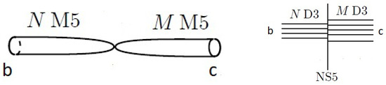
Figure 12. The cigars of the Taub-NUT space of 11-dimensional spacetime that are wrapped by the branes (left). The brane system of the Type IIB theory (right). The labels b and c are the asymptotic boundary conditions taking values in $H_1{(M^3;\mathbb{Z})}^N\times H_1{(M^3;\mathbb{Z})}^M$ for $U\left(N\right|M)$.

The M5 branes are transformed into D4 branes. The D6 brane appears as a consequence of the Taub-NUT space. We apply T-duality along $S_{\mathrm{t}}^1$ to pass to type IIB. And then we apply S-duality. We arrive at the following final brane system shown in Figure 12:

Type IIB 10D ST	$S^1$	×	$T^{\ast }{M}^3$	×	${\mathbb{R}}^3$
1 NS5 brane	pt	×	$T^{\ast }{M}^3$	×	$\left\{0\right\}$
M D3 branes	pt	×	$M^3$	×	${\mathbb{R}}_{+}$
N D3 branes	pt	×	$M^3$	×	${\mathbb{R}}_{-}$

The S-duality maps the D5 brane to NS5 brane. The former was obtained from the above D6 brane. On the stack of the D3 branes, its world-volume theory is $4d\mathcal{N}=4$ super Yang–Mills with gauge groups $U\left(M\right)$, whereas the theory on the other brane stack has gauge group $U\left(N\right)$.

We next apply the (GL) topological twist along $M^3$ of $T^{\ast }{M}^3$ to the above super Yang–Mills theories [119]. This results in a cohomological quantum field theory that is a coupled 4d-3d system across the NS5 brane. The cohomological sector of the theory is the Chern–Simons theory based on $U\left(N\right|M)$ (up to Q-exact terms). Its action functional is the supergroup Chern–Simons theory (up to certain exact terms). Furthermore, analogous to the Chern–Simons level parameter in case of a Lie group $SU\left(N\right)$, $U\left(N\right|M)$ Chern–Simons theory carries a parameter K, which comes from the complexified gauge coupling constant $\tau$ of the super Yang–Mills theory, which in turn comes from the complexified string coupling constant.

$$\tau =Kcos\left(\theta \right)e^{i\theta }\in H^{+},$$

where $\theta$ is the vacuum angle and $H^{+}$ the upper half of the complex plane ($Im\tau >0$). $U\left(N\right|M)$ Chern–Simons theory is supported on $M^3$ in the NS5 brane. Its action functional at level K is

$$CS\left(\mathcal{A}\right)={\displaystyle \frac{iK}{4\pi }}{\int }_{M^3}Str\left(\mathcal{A}d\mathcal{A}+{\displaystyle \frac{2}{3}}{\mathcal{A}}^3\right)+\left\{Q,\cdots \right\},$$

where $\mathcal{A}={\mathcal{A}}_b+{\mathcal{A}}_f,{\mathcal{A}}_f$ is a fermion field, and ${\mathcal{A}}_b$ is the complexified gauge connection of A:

$${\mathcal{A}}_b=\left(A+isin\left(\theta \right)\varphi \right){|}_{y=0^{\pm }},$$

The + sign provides the $G_r$-part of ${\mathcal{A}}_b$ whereas the − sign provides the $G_l$-part of ${\mathcal{A}}_b$ (Recall that the bosonic (Grassman even) part of $U\left(N\right|M)$ is $U\left(N\right)\oplus U\left(M\right)$).

The existence of super ${\widehat{Z}}_{b,c}$ can be predicted from 11 dimensions. Specifically, the presence of the cigars in Figure 12, in particular their geometry away from the tips, requires imposing (asymptotic) boundary conditions $(b,c)\in H_1{(M^3;\mathbb{Z})}^N\times H_1{(M^3;\mathbb{Z})}^M$. The partition function over the BPS sector of the Hilbert space of the brane system is

$${\widehat{Z}}_{b,c}^{gl\left(N\right|M)}[M^3;q]:=T{r}_{H_{b,c}}{(-1)}^F{q}^{L_0}.$$

where F is the fermion number operator and $L_0$ is the generator of $U{\left(1\right)}_q$.

5. Super Series for Knot Complements

Motivated by the idea of partial surgery (29), a generalization of (56) to complements of plumbed knots was analyzed in [66]. We found that a series invariant of plumbed knot complement associated with $sl\left(2\right|1)$ is a three-variable series. Specifically, it is sum of contributions from good chambers ${\alpha }_{\pm }$.

$$F_K(y,z,q):=F_K(y,z,q;{\alpha }_{+})+F_K(y,z,q;{\alpha }_{-}),$$

The general form of super $F_K$ is

$$F_K(y,z,q)=c+\sum _{\begin{array}{c}m,n\in {\mathbb{Z}}_{\ge 0}^2\\ (m,n)\ne (0,0)\end{array}}{f}_{m,n}(K;q)\left({\displaystyle \frac{y^m}{z^n}}-{\displaystyle \frac{z^n}{y^m}}\right)\in \mathbb{Z}+q^{\Delta }\mathbb{Z}[q^{-1},q]]\left[[y/z,{(y/z)}^{-1}]\right].$$

(55)

It carries the Weyl symmetry $y\leftrightarrow y^{-1}$ and $z\leftrightarrow z^{-1}$. In comparison with (23), the summation of (23) is over odd integers, whereas (55) is over a pair of nonzero integers.

5.1. Torus Knots

We use the plumbing graph descriptions of torus knots in Section 3.1 to find good chambers for infinite families of torus knots.

Proposition  6

([66]). Let v be the number of vertices of plumbing graphs of $T(2,2n+1)$ and $T(3,3n+w),w=1,2$, and ${\alpha }_{+}=({\alpha }_1,{\alpha }_2,{\alpha }_{v-1})$ and ${\alpha }_{-}$ be the good chambers for torus knots, where ${\alpha }_1$ corresponds to degree-three vertex and the other two are associated with degree-one vertices of their plumbing graphs. Their good chambers, given by

$${\alpha }_{+}=(1,1,1),{\alpha }_{-}=-{\alpha }_{+},$$

yield a well-defined (Laurent) power series $f_{m,n}\left(q\right)$.

The general structure of the super $F_K$ of torus knots $K=T(2,2l+1),l\ge 2$ splits into q-independent and -dependent parts. The former is a new feature in super $F_K$, which is absent in (23). And it can be expressed in terms of the unknot. The latter has the following form:

$$\sum _{(m,n)\in {\mathbb{Z}}_{+}^2}{ϵ}_{m,n}{q}^{{\displaystyle \frac{m(m+g(m,n\left)\right)}{2(2l+1)}}}\left({\displaystyle \frac{y^m}{z^{m+g(m,n)}}}+{\displaystyle \frac{y^{m+g(m,n)}}{z^m}}-{\displaystyle \frac{z^m}{y^{m+g(m,n)}}}-{\displaystyle \frac{z^{m+g(m,n)}}{y^m}}\right),$$

where $g(m,n;K)=g(m,n)\in \left\{1,3,5,\cdots ,2l-1\right\}$ and ${ϵ}_{m,n}\left(K\right)={ϵ}_{m,n}$ is a sign function (see [66] for its algorithm).

We list a few examples of torus knots (additional examples are recorded in [66]).

$$F_{T(2,3)}(y,z,q)=1+\sum _{i=2}^{\infty }\left(y^i+{\displaystyle \frac{1}{z^i}}\right)-\sum _{i=2}^{\infty }\left({\displaystyle \frac{1}{y^i}}+z^i\right)+q\left({\displaystyle \frac{y^2}{z^3}}+{\displaystyle \frac{y^3}{z^2}}-{\displaystyle \frac{z^2}{y^3}}-{\displaystyle \frac{z^3}{y^2}}\right)$$

$$+q^2\left({\displaystyle \frac{y^3}{z^4}}+{\displaystyle \frac{y^4}{z^3}}-{\displaystyle \frac{z^3}{y^4}}-{\displaystyle \frac{z^4}{y^3}}\right)+q^5\left(-{\displaystyle \frac{y^5}{z^6}}-{\displaystyle \frac{y^6}{z^5}}+{\displaystyle \frac{z^5}{y^6}}+{\displaystyle \frac{z^6}{y^5}}\right)+q^7\left(-{\displaystyle \frac{y^6}{z^7}}-{\displaystyle \frac{y^7}{z^6}}+{\displaystyle \frac{z^6}{y^7}}+{\displaystyle \frac{z^7}{y^6}}\right)$$

$$+q^{12}\left({\displaystyle \frac{y^8}{z^9}}+{\displaystyle \frac{y^9}{z^8}}-{\displaystyle \frac{z^8}{y^9}}-{\displaystyle \frac{z^9}{y^8}}\right)+q^{15}\left({\displaystyle \frac{y^9}{z^{10}}}+{\displaystyle \frac{y^{10}}{z^9}}-{\displaystyle \frac{z^9}{y^{10}}}-{\displaystyle \frac{z^{10}}{y^9}}\right)+\cdots$$

$$F_{T(2,5)}(y,z,q)=1+\sum _{\begin{array}{c}i=2\\ i\ne 3\end{array}}^{\infty }\left(y^i+{\displaystyle \frac{1}{z^i}}\right)-\sum _{\begin{array}{c}i=2\\ i\ne 3\end{array}}^{\infty }\left({\displaystyle \frac{1}{y^i}}+z^i\right)+q\left({\displaystyle \frac{y^2}{z^5}}+{\displaystyle \frac{y^5}{z^2}}-{\displaystyle \frac{z^2}{y^5}}-{\displaystyle \frac{z^5}{y^2}}\right)$$

$$+q^2\left({\displaystyle \frac{y^4}{z^5}}+{\displaystyle \frac{y^5}{z^4}}-{\displaystyle \frac{z^4}{y^5}}-{\displaystyle \frac{z^5}{y^4}}\right)+q^3\left({\displaystyle \frac{y^5}{z^6}}+{\displaystyle \frac{y^6}{z^5}}-{\displaystyle \frac{z^5}{y^6}}-{\displaystyle \frac{z^6}{y^5}}\right)+q^4\left({\displaystyle \frac{y^5}{z^8}}+{\displaystyle \frac{y^8}{z^5}}-{\displaystyle \frac{z^5}{y^8}}-{\displaystyle \frac{z^8}{y^5}}\right)$$

$$+q^7\left(-{\displaystyle \frac{y^7}{z^{10}}}-{\displaystyle \frac{y^{10}}{z^7}}+{\displaystyle \frac{z^7}{y^{10}}}+{\displaystyle \frac{z^{10}}{y^7}}\right)+q^9\left(-{\displaystyle \frac{y^9}{z^{10}}}-{\displaystyle \frac{y^{10}}{z^9}}+{\displaystyle \frac{z^9}{y^{10}}}+{\displaystyle \frac{z^{10}}{y^9}}\right)+\cdots$$

$$F_{T(3,4)}(y,z,q)=1+\sum _{\begin{array}{c}i=3\\ i\ne 5\end{array}}^{\infty }\left(y^i+{\displaystyle \frac{1}{z^i}}\right)-\sum _{\begin{array}{c}i=3\\ i\ne 5\end{array}}^{\infty }\left({\displaystyle \frac{1}{y^i}}+z^i\right)+q\left({\displaystyle \frac{y^3}{z^4}}+{\displaystyle \frac{y^4}{z^3}}-{\displaystyle \frac{z^3}{y^4}}-{\displaystyle \frac{z^4}{y^3}}\right)$$

$$+q^2\left({\displaystyle \frac{y^3}{z^8}}+{\displaystyle \frac{y^4}{z^6}}+{\displaystyle \frac{y^6}{z^4}}+{\displaystyle \frac{y^8}{z^3}}-{\displaystyle \frac{z^3}{y^8}}-{\displaystyle \frac{z^4}{y^6}}-{\displaystyle \frac{z^6}{y^4}}-{\displaystyle \frac{z^8}{y^3}}\right)+q^3\left({\displaystyle \frac{y^4}{z^9}}+{\displaystyle \frac{y^9}{z^4}}-{\displaystyle \frac{z^4}{y^9}}-{\displaystyle \frac{z^9}{y^4}}\right)+q^4\left({\displaystyle \frac{y^6}{z^8}}+{\displaystyle \frac{y^8}{z^6}}-{\displaystyle \frac{z^6}{y^8}}-{\displaystyle \frac{z^8}{y^6}}\right)$$

$$+q^6\left({\displaystyle \frac{y^8}{z^9}}+{\displaystyle \frac{y^9}{z^8}}-{\displaystyle \frac{z^8}{y^9}}-{\displaystyle \frac{z^9}{y^8}}\right)+q^7\left(-{\displaystyle \frac{y^7}{z^{12}}}-{\displaystyle \frac{y^{12}}{z^7}}+{\displaystyle \frac{z^7}{y^{12}}}+{\displaystyle \frac{z^{12}}{y^7}}\right)+q^{10}\left(-{\displaystyle \frac{y^{10}}{z^{12}}}-{\displaystyle \frac{y^{12}}{z^{10}}}+{\displaystyle \frac{z^{10}}{y^{12}}}+{\displaystyle \frac{z^{12}}{y^{10}}}\right)$$

$$+q^{11}\left(-{\displaystyle \frac{y^{11}}{z^{12}}}-{\displaystyle \frac{y^{12}}{z^{11}}}+{\displaystyle \frac{z^{11}}{y^{12}}}+{\displaystyle \frac{z^{12}}{y^{11}}}\right)+q^{13}\left(-{\displaystyle \frac{y^{12}}{z^{13}}}-{\displaystyle \frac{y^{13}}{z^{12}}}+{\displaystyle \frac{z^{12}}{y^{13}}}+{\displaystyle \frac{z^{13}}{y^{12}}}\right)+q^{14}\left(-{\displaystyle \frac{y^{12}}{z^{14}}}-{\displaystyle \frac{y^{14}}{z^{12}}}+{\displaystyle \frac{z^{12}}{y^{14}}}+{\displaystyle \frac{z^{14}}{y^{12}}}\right)$$

$$+q^{17}\left(-{\displaystyle \frac{y^{12}}{z^{17}}}-{\displaystyle \frac{y^{17}}{z^{12}}}+{\displaystyle \frac{z^{12}}{y^{17}}}+{\displaystyle \frac{z^{17}}{y^{12}}}\right)+\cdots$$

5.2. The Dehn Surgery Formula

We provide the Dehn surgery formula relating super $F_K$ to super ${\widehat{Z}}_{b,c}$.

Theorem  11

([66]). Let $Y_K$ be the complement of a knot K in the 3-sphere $S^3$, and let $Y_{p/r}$ be a result of Dehn surgery along K with slope $p/r\in {\mathbb{Q}}^{\ast }$. Assume that $Y_K$ and $Y_{p/r}$ are represented by negative definite plumbings. Then the invariants of $Y_{p/r}$ are given by

$${\widehat{Z}}_{b,c}[Y_{p/r};q]={(-1)}^{\tau }{\mathcal{L}}_{b,c}^{({\alpha }_i;p/r)}\left[F_K^{\left({\alpha }_i\right)}(y,z,q)\right],$$

where the Laplace transform for the ${\alpha }_{+}$ chamber is

$${\mathcal{L}}_{b,c}^{({\alpha }_{+};p/r)}:y^{\alpha }{z}^{\beta }{q}^{\gamma }\mapsto q^{\gamma }\left\{\begin{array}{cc}{\displaystyle \sum _{r_s=r_{s,min}}^{\infty }}{q}^{{\displaystyle \frac{\beta (r\alpha +ϵr_s)}{p}}},\hfill & \mathit{if}r\alpha +ϵr_s+b\in p\mathbb{Z},r\beta +c\in p\mathbb{Z}\hfill \\ {\displaystyle \sum _{w_s=w_{s,min}}^{\infty }}{q}^{{\displaystyle \frac{\alpha (r\beta -ϵw_s)}{p}}},\hfill & \mathit{if}r\beta -ϵw_s+c\in p\mathbb{Z},r\alpha +b\in p\mathbb{Z}\hfill \\ 0,\hfill & \mathit{otherwise}\hfill \end{array}\right.$$

And the Laplace transform for the ${\alpha }_{-}$ chamber is

$${\mathcal{L}}_{b,c}^{({\alpha }_{-};p/r)}:y^{\alpha }{z}^{\beta }{q}^{\gamma }\mapsto -q^{\gamma }\left\{\begin{array}{cc}{\displaystyle \sum _{w_s^{\prime }=w_{s,min}^{\prime }}^{\infty }}{q}^{{\displaystyle \frac{\beta (r\alpha -ϵw_s^{\prime })}{p}}},\hfill & \mathit{if}r\alpha -ϵw_s^{\prime }+b\in p\mathbb{Z},r\beta +c\in p\mathbb{Z}\hfill \\ {\displaystyle \sum _{r_s^{\prime }=r_{s,min}^{\prime }}^{\infty }}{q}^{{\displaystyle \frac{\alpha (r\beta +ϵr_s^{\prime })}{p}}},\hfill & \mathit{if}r\beta +ϵr_s^{\prime }+c\in p\mathbb{Z},r\alpha +b\in p\mathbb{Z}\hfill \\ 0,\hfill & \mathit{otherwise}\hfill \end{array}\right.$$

where $r_{s,min},r_{s,min}^{\prime }\ge 1,w_{s,min},w_{s,min}^{\prime }\ge 0$, and $ϵ=sign\left(p\right){(-1)}^{\pi +1}$.

We observe a qualitative difference between the above surgery formula and $sl\left(2\right)$ surgery formula (33) in Section 3.5. For applications of Theorem 11, $S_{-1/r}^3\left(T(s,t)\right)$ and $S_{-p}^3\left(T(s,t)\right)$ for some values of $s,t,r,p$, and $S_{-p}^3\left(unknot\right)$ were considered in [66].

6. Future Directions

We list open problems:

• Obtaining an analytic formula of ${\widehat{Z}}_b\left(q\right)$ defined on $\left|q\right|>1$ for positive definite plumbed manifolds $-Y_{\Gamma }$ has been a major challenge. Several approaches for computing ${\widehat{Z}}_b(-Y_{\Gamma },q)$ are listed in Section 2.7. However, they are applicable to specific examples of $-Y_{\Gamma }$.
• There are multiple Dehn surgery formulas (cf. Section 3.5). Each has restricted applicability. We believe that a unifying surgery formula exists and would be important.
• Extending the definition of $F_L$ beyond homogeneous links would be valuable conceptually and computationally.
• A construction of ${\mathcal{H}}_{BPS}$ in Section 2.2 for categorification of the WRT invariant is highly desirable.

References

- Nawata, S.; Ramadevi, P. Zodinmawia, Colored HOMFLY polynomials from Chern-Simons theory. J. Knot Theory Ramif. 2013, 22, 1350078. [Google Scholar] [CrossRef]
- Witten, E. Quantum field theory and the Jones polynomial. Comm. Math. Phys. 1989, 121, 351–399. [Google Scholar] [CrossRef]
- Witten, E. Topological quantum field theory. Comm. Math. Phys. 1988, 117, 353–386. [Google Scholar] [CrossRef]
- Witten, E. Monopoles and Four-Manifolds. Math. Res. Lett. 1994, 1, 769–796. [Google Scholar] [CrossRef]
- Reshetikhin, N.; Turaev, V. Invariants of 3-manifolds via link polynomials and quantum groups. Invent. Math. 1991, 103, 547–597. [Google Scholar] [CrossRef]
- Reshetikhin, N.; Turaev, V. Ribbon graphs and their invariants derived from quantum groups. Comm. Math. Phys. 1990, 127, 1–26. [Google Scholar] [CrossRef]
- Kirby, R.; Melvin, P. The 3-manifold invariants of Witten and Reshetikhin-Turaev for sl(2,C). Invent. Math. 1991, 105, 473–545. [Google Scholar] [CrossRef]
- Atiyah, M. Topological quantum field theory. Publ. Math. l’I.H.É.S. 1988, 68, 175–186. [Google Scholar] [CrossRef]
- Segal, G. The Definition of Conformal Field Theory. In Differential Geometrical Methods in Theoretical Physics; NATO ASI Series; Springer: Berlin/Heidelberg, Germany, 1988. [Google Scholar]
- Freed, D. Lectures on Field Theory and Topology; American Mathematical Society: Providence, RI, USA, 2019; p. 133. [Google Scholar]
- Baez, J.; Dolan, J. Higher dimensional algebra and topological quantum field theory. J. Math. Phys. 1995, 36, 6073. [Google Scholar] [CrossRef]
- Freed, D. Remarks on Fully Extended 3-Dimensional Topological Field Theories. Available online: https://www2.math.upenn.edu/StringMath2011/notes/Freed_StringMath2011_talk.pdf (accessed on 2 December 2025).
- Schommer-Pries, C. The Classification of Two-Dimensional Extended Topological Field Theories. arXiv 2011, arXiv:1112.1000. [Google Scholar]
- Lurie, J. On the classification of topological field theories. Curr. Dev. Math. 2009, 2009, 129–280. [Google Scholar] [CrossRef]
- Akutsu, Y.; Deguchi, T.; Ohtsuki, T. Invariants of colored links. J. Knot Theory Ramif. 1992, 1, 161–184. [Google Scholar] [CrossRef]
- Murakami, J. Colored alexander invariants and cone-manifolds. Osaka J. Math. 2008, 45, 541–564. [Google Scholar]
- Geer, N.; Kujawa, J.; Patureau-Mirand, B. Ambidextrous objects and trace functions for nonsemisimple categories. Proc. Amer. Math. Soc. 2013, 141, 9. [Google Scholar] [CrossRef]
- Geer, N.; Kujawa, J.; Patureau-Mirand, B. Generalized trace and modified dimension functions on ribbon categories. Sel. Math. 2011, 17, 453–504. [Google Scholar] [CrossRef]
- Geer, N.; Patureau-Mirand, B.; Turaev, V. Modified quantum dimensions and re-normalized link invariants. Compos. Math. 2009, 145, 196–212. [Google Scholar] [CrossRef]
- Costantino, F.; Geer, N.; Patureau-Mirand, B. Quantum invariants of 3-manifolds via link surgery presentations and non-semi-simple categories. J. Topol. 2014, 7, 1005–1053. [Google Scholar] [CrossRef]
- Geer, N.; Patureau-Mirand, B. Multivariable link invariants arising from sl(2|1) and the Alexander polynomial. J. Pure Appl. Algebra 2007, 210, 283–298. [Google Scholar] [CrossRef]
- Geer, N.; Patureau-Mirand, B. Multivariable link invariants arising from Lie superalgebras of type I. J. Knot Theory Ramif. 2010, 19, 93–115. [Google Scholar] [CrossRef]
- Ha, N.P. Topological invariants from quantum group Uζ(sl(2|1)) at roots of unity. arXiv 2016, arXiv:1607.03728. [Google Scholar]
- Crane, L.; Frenkel, I.B. Four dimensional topological quantum field theory, Hopf categories, and the canonical bases. J. Math. Phys. 1994, 35, 5136. [Google Scholar] [CrossRef]
- Aganagic, M. Homological knot invariants from mirror symmetry. Proc. Int. Cong. Math. 2022, 3, 2108–2144. [Google Scholar]
- Gukov, S. Gauge theory and knot homologies. Fortschr. Phys. 2007, 55, 473–490. [Google Scholar] [CrossRef]
- Nawata, S.; Oblomkov, A. Lectures on knot homology. arXiv 2015, arXiv:1510.01795. [Google Scholar]
- Stroppel, C. Categorification: Tangle invariants and TQFTs. Proc. Int. Cong. Math. 2022, 2, 1312–1353. [Google Scholar]
- Ozsvath, P.; Szabo, Z. Holomorphic disks and knot invariants. Adv. Math. 2004, 186, 58–116. [Google Scholar] [CrossRef]
- Ozsvath, P.; Szabo, Z. Holomorphic disks, link invariants and the multi-variable Alexander polynomial. Alg. Geom. Topol. 2008, 8, 615–692. [Google Scholar] [CrossRef]
- Rasmussen, J. Floer homology and knot complements. arXiv 2022, arXiv:math/0306378. [Google Scholar]
- Khovanov, M. A categorification of the Jones polynomial. Duke Math. J. 2003, 101, 359–426. [Google Scholar] [CrossRef]
- Khovanov, M. A categorification of the colored Jones polynomial. J. Knot Theory Ramif. 2005, 14, 111–130. [Google Scholar] [CrossRef]
- Khovanov, M.; Rozansky, L. Matrix factorizations and link homology 2. Geom. Topol. 2008, 12, 1387–1425. [Google Scholar] [CrossRef]
- Khovanov, M.; Lauda, A. A diagrammatic approach to categorification of quantum groups I. Represent. Theory 2009, 13, 309–347. [Google Scholar]
- Lauda, A. An introduction to diagrammatic algebra and categorified quantum sl(2). arXiv 2011, arXiv:1106.2128. [Google Scholar] [CrossRef]
- Ooguri, H.; Vafa, C. Knot Invariants and Topological Strings. Nuclear Phys. B 2000, 577, 419–438. [Google Scholar] [CrossRef]
- Gukov, S.; Schwarz, A.; Vafa, C. Khovanov-Rozansky Homology and Topological Strings. Letters Math. Phys. 2005, 74, 53–74. [Google Scholar] [CrossRef]
- Khovanov, M.; Rozansky, L. Matrix factorizations and link homology 1. Fund. Math. 2008, 199, 1–91. [Google Scholar] [CrossRef]
- Khovanov, M. sl(3) link homology. Algebr. Geom. Topol. 2004, 4, 1045–1081. [Google Scholar] [CrossRef]
- Gukov, S.; Nawata, S.; Saberi, I.; Stosic, M.; Sulkowski, P. Sequencing BPS spectra. J. High Energ. Phys. 2016, 2016, 4. [Google Scholar] [CrossRef]
- Witten, E. Fivebranes and Knots. Quantum Topol. 2012, 3, 1–137. [Google Scholar] [CrossRef]
- Witten, E. Khovanov Homology And Gauge Theory. arXiv 2011, arXiv:1108.3103. [Google Scholar]
- Witten, E. Two Lectures on Gauge Theory and Khovanov Homology. arXiv 2016, arXiv:1603.03854. [Google Scholar]
- Elias, B.; Qi, Y. Categorification of quantum sl(2) at prime roots of unity. Adv. Math. 2016, 299, 863–930. [Google Scholar] [CrossRef][Green Version]
- Khovanov, M. Hopfological algebra and categorification at a root of unity: The first steps. J. Knot Theory Ramif. 2016, 25, 1640006. [Google Scholar] [CrossRef]
- Gukov, S.; Putrov, P.; Vafa, C. Fivebranes and 3-manifold homology. J. High Energ. Phys. 2017, 7, 71. [Google Scholar] [CrossRef]
- Gukov, S.; Pei, D.; Putrov, P.; Vafa, C. BPS spectra and 3-manifold invariants. J. Knot Theory Ramif. 2020, 29, 2040003. [Google Scholar]
- Lawrence, R.; Zagier, D. Modular forms and quantum invariants of 3-manifolds. Asian J. Math. 1999, 3, 93–107. [Google Scholar] [CrossRef]
- Murakami, Y. A Proof of a Conjecture of Gukov–Pei–Putrov–Vafa. Commun. Math. Phys. 2024, 405, 274. [Google Scholar] [CrossRef]
- Gukov, S.; Manolescu, C. A two-variable series for knot complements. Quantum Topol. 2021, 12, 1–109. [Google Scholar] [CrossRef]
- Park, S. Higher Rank and FK. SIGMA 2020, 16, 44. [Google Scholar]
- Cheng, M.; Chun, S.; Ferrari, F.; Gukov, S.; Harrison, S.M. 3d modularity. J. High Energ. Phys. 2019, 2019, 10. [Google Scholar] [CrossRef]
- Cheng, M.; Coman, I.; Kucharski, P.; Passaro, D.; Sgroi, G. 3d Modularity Revisited. arXiv 2024, arXiv:2403.14920. [Google Scholar] [CrossRef]
- Chae, J. Witt invariants from q-series. Lett. Math. Phys. 2023, 113, 3. [Google Scholar] [CrossRef]
- Gukov, S.; Putrov, P.; Park, S. Cobordism invariants from BPS q-series. Ann. Henri Poincare 2021, 22, 4173–4203. [Google Scholar] [CrossRef]
- Gruen, A. The sl(N) Symmetrically Large Coloured R Matrix. arXiv 2022, arXiv:2212.05222. [Google Scholar]
- Park, S. Large color R-matrix for knot complements and strange identities. J. Knot Theory Ramif. 2020, 29, 2050097. [Google Scholar]
- Park, S. Inverted state sums, inverted Habiro series, and indefinite theta functions. arXiv 2021, arXiv:2106.03942. [Google Scholar] [CrossRef]
- Ekholm, T.; Gruen, A.; Gukov, S.; Kucharski, P.; Park, S.; Stošić, M.; Sułkowski, P. Branches, quivers, and ideals for knot complements. arXiv 2021, arXiv:2110.13768. [Google Scholar] [CrossRef]
- Akhmechet, R.; Johnson, P.; Krushkal, V. Lattice cohomology and q-series invariants of 3-manifolds. arXiv 2021, arXiv:2109.14139. [Google Scholar] [CrossRef]
- Liles, L.; McSpirit, E. Infinite families of quantum modular 3-manifold invariants. arXiv 2023, arXiv:2306.14765. [Google Scholar] [CrossRef]
- Akhmechet, R.; Johnson, P.; Park, S. Knot lattice homology and q-series invariants for plumbed knot complements. arXiv 2024, arXiv:2403.14461. [Google Scholar] [CrossRef] [PubMed]
- Moore, A.; Tarasca, N. Root lattices and invariant series for plumbed 3-manifolds. arXiv 2024, arXiv:2405.14972. [Google Scholar]
- Ferrari, F.; Putrov, P. Supergroups, q-series and 3-manifolds. Ann. Henri Poincare 2024, 25, 2781–2837. [Google Scholar] [CrossRef]
- Chae, J. A supergroup series for knot complements. arXiv 2025, arXiv:2508.10279. [Google Scholar] [CrossRef]
- Fenn, R.; Rourke, C. On Kirby’s calculus of links. Topology 1979, 18, 1–15. [Google Scholar] [CrossRef]
- Kirby, R. A calculus for framed links in S3. Invent. Math. 1978, 45, 35–56. [Google Scholar] [CrossRef]
- Neumann, W. A calculus for plumbing applied to the topology of complex surface singularities and degenerating complex curves. Trans. Amer. Math. Soc. 1981, 268, 299–344. [Google Scholar] [CrossRef]
- Neumann, W.; Raymond, F. Seifert manifolds, plumbing, μ-invariant and orientation reversing maps. In Proceedings of the Symposium at Santa Barbara, Santa Barbara, CA, USA, 25–29 July 1977. [Google Scholar]
- Chun, S.; Gukov, S.; Park, S.; Sopenko, N. 3d-3d correspondence for mapping tori. J. High Energ. Phys. 2020, 2020, 152. [Google Scholar] [CrossRef]
- Gukov, S.; Katzarkov, L.; Svoboda, J. for plumbed manifolds and splice diagrams. arXiv 2023, arXiv:2304.00699. [Google Scholar]
- Dimofte, T.; Gaiotto, D.; Gukov, S. Gauge Theories Labelled by Three-Manifolds. Commun. Math. Phys. 2014, 325, 367–419. [Google Scholar] [CrossRef]
- Dimofte, T.; Gaiotto, D.; Gukov, S. 3-Manifolds and 3d Indices. Adv. Theor. Math. Phys. 2013, 17, 975–1076. [Google Scholar] [CrossRef]
- Bringmann, K.; Mahlburg, K.; Milas, A. Higher depth quantum modular forms and plumbed 3-manifolds. Lett. Math. Phys. 2020, 110, 2675–2702. [Google Scholar] [CrossRef]
- Zagier, D. Quantum Modular Forms. Clay Math. Proc. 2010, 2010, 12. [Google Scholar]
- Chung, H.-J. BPS invariants for Seifert manifolds. J. High Energ. Phys. 2020, 2020, 113. [Google Scholar] [CrossRef]
- Chung, H.-J. BPS invariants for a Knot in Seifert manifolds. J. High Energ. Phys. 2022, 2022, 122. [Google Scholar] [CrossRef]
- Cheng, M.; Chun, S.; Feigin, B.; Ferrari, F.; Gukov, S.; Harrison, S.M.; Passaro, D. 3-Manifolds and VOA Characters. Commun. Math. Phys. 2024, 405, 44. [Google Scholar] [CrossRef]
- Gukov, S.; Jagadale, M. ceff for 3d N = 2 theories. arXiv 2023, arXiv:2308.05360. [Google Scholar] [CrossRef]
- Adams, G.; Costin, O.; Dunne, G.; Gukov, S.; Oner, O. ceff from Resurgence at the Stokes Line. arXiv 2025, arXiv:2508.10112v1. [Google Scholar]
- Harichurn, S.; Jagadale, M.; Noshchenko, D.; Passaro, D. ceff from surgery and modularity. arXiv 2025, arXiv:2508.10087v1. [Google Scholar]
- Rokhlin, V. New results in the theory of four-dimensional manifolds. Doklady Acad. Nauk. 1952, 84, 221–224. [Google Scholar]
- Harichurn, S.; Nemethi, A.; Svoboda, J. Delta invariants of plumbed 3-manifolds. arXiv 2024, arXiv:2412.02042v1. [Google Scholar] [CrossRef]
- Nemethi, A.; Nicolaescu, L. Seiberg–Witten invariants and surface singularities. Geom. Topol. 2002, 6, 269–328. [Google Scholar] [CrossRef][Green Version]
- Costantino, F.; Gukov, S.; Putrov, P. Non-Semisimple TQFT’S and BPS q-series. SIGMA 2023, 19, 10. [Google Scholar] [CrossRef]
- Kirby, R.; Melvin, P.; Zhang, X. Quantum invariants at the sixth root of unity. Commun. Math. Phys. 1993, 151, 607–617. [Google Scholar] [CrossRef]
- Casson, A.; Gordon, C. On slice knots in dimension three. Proc. Symp. Pure Math. 1978, 32, 39–53. [Google Scholar]
- Milnor, J.; Husemoller, D. Symmetric Bilinear Forms. In A Series of Modern Surveys in Mathematics; Springer: Berlin/Heidelberg, Germany, 1973. [Google Scholar]
- Zwegers, S. Mock Theta Functions. Ph.D. Thesis, University of Utrecht, Utrecht, The Netherlands, 2002. [Google Scholar]
- Costin, O.; Dunne, G.; Gruen, A.; Gukov, S. Going to the Other Side via the Resurgent Bridge. arXiv 2023, arXiv:2310.12317. [Google Scholar] [CrossRef]
- Gukov, S.; Marino, M.; Putrov, P. Resurgence in complex Chern-Simons theory. arXiv 2016, arXiv:1605.07615. [Google Scholar] [CrossRef]
- Cheng, M.; Ferrari, F.; Sgroi, G. Three-manifold quantum invariants and mock theta functions. Philos. Trans. Roy. Soc. A 2018, 378, 20180439. [Google Scholar] [CrossRef]
- Habiro, K. On the quantum sl2 invariants of knots and integral homology spheres. Geom. Topol. Monogr. 2002, 4, 55–68. [Google Scholar]
- Svoboda, J. Inverted Habiro Series and its Residues. arXiv 2025, arXiv:2509.22610. [Google Scholar] [CrossRef]
- Lickorish, W. A Representation of Orientable Combinatorial 3-Manifolds. Ann. Math. 1962, 76, 531–540. [Google Scholar] [CrossRef]
- Wallace, A. Modifications and Cobounding Manifolds. Can. J. Math. 1960, 12, 503–528. [Google Scholar] [CrossRef]
- Guicardi, P.; Jagadale, M. -TQFT, Surgery Formulas, and New Algebras. arXiv 2025, arXiv:2509.14311. [Google Scholar]
- Melvin, P.; Morton, H. The coloured Jones function. Commun. Math. Phys. 1995, 169, 501–520. [Google Scholar] [CrossRef]
- Rozansky, L. Higher order terms in the Melvin-Morton expansion of the colored Jones polynomial. Commun. Math. Phys. 1997, 183, 291–306. [Google Scholar] [CrossRef]
- Rozansky, L. The Universal R-Matrix, Burau Representaion and the Melvin-Morton Expansion of the Colored Jones Polynomial. Adv. Math 1998, 134, 1–31. [Google Scholar] [CrossRef][Green Version]
- Bar-Natan, D.; Garoufalidis, S. On the Melvin-Morton-Rozansky conjecture. Invent. Math. 1996, 125, 103–133. [Google Scholar] [CrossRef]
- Gruen, A.; Suarez, L. A large color R-matrix for sl3. arXiv 2025, arXiv:2508.15171. [Google Scholar]
- Garoufalidis, S.; Le, T. The colored Jones function is q–holonomic. Geom. Topol. 2005, 9, 1253–1293. [Google Scholar] [CrossRef]
- Gukov, S. Three-Dimensional Quantum Gravity, Chern-Simons Theory, and the A-Polynomial. Commun. Math. Phys. 2005, 255, 577–627. [Google Scholar] [CrossRef]
- Gukov, S.; Hsin, P.-S.; Nakajima, H.; Park, S.; Pei, D.; Sopenko, N. Rozansky-Witten geometry of Coulomb branches and logarithmic knot invariants. J. Geom. Phys. 2021, 168, 104311. [Google Scholar] [CrossRef]
- Chae, J. Knot Complement, ADO Invariants and their Deformations for Torus Knots. SIGMA 2020, 16, 134. [Google Scholar] [CrossRef]
- Ekholm, T.; Gruen, A.; Gukov, S.; Kucharski, P.; Park, S.; Sulkowski, P. at large N: From curve counts to quantum modularity. Commun. Math. Phys. 2022, 396, 143–186. [Google Scholar] [CrossRef]
- Dunfield, N.; Gukov, S.; Rasmussen, J. The Superpolynomial for Knot Homologies. Exp. Math. 2006, 15, 129–160. [Google Scholar] [CrossRef]
- Fuji, H.; Gukov, S.; Stosic, M.; Sulkowski, P. 3d analogs of Argyres-Douglas theories and knot homologies. J. High Energ. Phys. 2013, 2013, 175. [Google Scholar] [CrossRef]
- Kucharski, P.; Reineke, M.; Stosic, M.; Sulkowski, P. BPS states, knots and quivers. Phys. Rev. D 2017, 96, 121902. [Google Scholar] [CrossRef]
- Kucharski, P.; Reineke, M.; Stosic, M.; Sulkowski, P. Knots-quivers correspondence. Adv. Theor. Math. Phys. 2019, 23, 1849–1902. [Google Scholar] [CrossRef]
- Kucharski, P. Quivers for 3-manifolds: The correspondence, BPS states, and 3d N = 2 theories. J. High Energy Phys. 2020, 9, 75. [Google Scholar] [CrossRef]
- Ekholm, T.; Kucharski, P.; Longhi, P. Multi-cover skeins, quivers, and 3d N = 2 dualities. J. High Energy Phys. 2020, 2, 18. [Google Scholar] [CrossRef]
- Chae, J. A Cable Knot and BPS-Series. SIGMA 2023, 19, 12. [Google Scholar] [CrossRef]
- Chae, J. A Cable Knot and BPS-Series II. Exp. Math. 2025, 34, 1–12. [Google Scholar] [CrossRef]
- Mikhaylov, V.; Witten, E. Branes and Supergroups. Commun. Math. Phys. 2015, 340, 699–832. [Google Scholar] [CrossRef]
- Vafa, C. Brane/anti-Brane Systems and U(N|M) Supergroup. arXiv 2001, arXiv:hep-th/0101218. [Google Scholar]
- Kapustin, A.; Witten, E. Electric-magnetic duality and the geometric Langlands program. Commun. Number Theory Phys. 2007, 1, 1–236. [Google Scholar] [CrossRef]
Disclaimer/Publisher’s Note: The statements, opinions and data contained in all publications are solely those of the individual author(s) and contributor(s) and not of MDPI and/or the editor(s). MDPI and/or the editor(s) disclaim responsibility for any injury to people or property resulting from any ideas, methods, instructions or products referred to in the content. |
© 2025 by the author. Licensee MDPI, Basel, Switzerland. This article is an open access article distributed under the terms and conditions of the Creative Commons Attribution (CC BY) license (https://creativecommons.org/licenses/by/4.0/).