Asymptotic Behavior of Solutions to the Nonlinear Schrödinger Equation with Non-Zero Boundary Conditions in the Presence of a Pair of Second-Order Discrete Spectra

Abstract

The nonlinear Schrödinger equation is a classical nonlinear evolution equation with wide applications. This paper explores the asymptotic behavior of solutions to the nonlinear Schrödinger equation with non-zero boundary conditions in the presence of a pair of second-order discrete spectra. We analyze the Riemann–Hilbert problem in the inverse scattering transform by the Deift–Zhou nonlinear steepest descent method. Then we propose a proper deformation to deal with the growing time term and give the conditions for the series in the process of deformation by the Laurent expansion. Finally, we provide the characterization of the interactions between the solitary waves corresponding to second-order discrete spectra and the coherent oscillations produced by the perturbation. Numerical verifications are also performed.

1. Introduction

1.1. Introduction to Nonlinear Schrödinger Equation

We consider the Schrödinger equation

$$\begin{array}{c}i{u}_t+u_{xx}+2{\left|u\right|}^{2}u=0,\\ {\displaystyle \underset{x\to \pm \infty }{lim}}u(x,t)=q_{\pm }{e}^{2i{q}_0^{2}t},\end{array}$$

(1)

where $|q_{\pm }|=q_0>0$. For simplicity, we substitute $u(x,t)=q(x,t)e^{2i{q}_0^{2}t}$ into (1) and get a convenient form

$$\begin{array}{c}i{q}_t+q_{xx}+{2\left(\right|q|}^2-q_0^2)q=0,\\ {\displaystyle \underset{x\to \pm \infty }{lim}}q(x,t)=q_{\pm }.\end{array}$$

(2)

The nonlinear Schrödinger Equation (2) can be reformulated in form of the compatibility condition of the Lax pair

$$\begin{array}{cc}\hfill {\phi }_x& =X\phi ,\hfill \\ \hfill {\phi }_t& =T\phi .\hfill \end{array}$$

(3)

where $\phi =\phi (x,t,k)$ is a 2 × 2 matrix-valued function, and

$$\begin{array}{cc}\hfill X(x,t,k)& =ik{P}_3+Q,\hfill \\ \hfill T(x,t,k)& =-2i{k}^2{P}_3+i{P}_3(Q_x-Q^2-q_0^{2}I)-2kQ,\hfill \\ \hfill P_3& =\left(\begin{array}{cc}1& 0\\ 0& -1\end{array}\right),\hfill \\ \hfill Q& =\left(\begin{array}{cc}0& q\\ -q^{*}& 0\end{array}\right).\hfill \end{array}$$

(4)

In the above, I is the $2\times 2$ identity matrix, $k\in \mathbb{C}$ is the spectral parameter and $q^{*}$ denotes the complex conjugate of q.

In fact, when (3) holds, the compatibility condition ${\left(X\phi \right)}_t={\left(T\phi \right)}_x$ leads to the nonlinear Schrödinger Equation (2) for $q(x,t)$, regardless of the value of k. Such treatment stems from the inverse scattering transform invented by Gardner et al. in 1967 for the Korteweg–de Vries equation [1]. Lax generalized it to integrable equations, and Zakharov and Shabat proved the integrability of the nonlinear Schrödinger equation [2], thus introducing the inverse scattering transform method into the study of this equation. The original inverse scattering transform method requires solving the Gelfand–Levitan–Marchenko integral equation [3,4]. Zakharov simplified the solution of the inverse scattering problem based on the Riemann–Hilbert problem [5].

The spectra of the inverse scattering transform refer to the set of all parameter values for which the eigenfunctions $\phi$ of the Lax pair are bounded. The spectra of the inverse scattering transform are defined in the complex plane and are divided into two types: discrete ones and continuous ones. The continuous spectrum corresponds to perturbations, while the discrete ones give rise to solitary waves. When both spectra coexist, the study of the asymptotic behavior of the equation solutions can help understand the properties of solutions to the nonlinear Schrödinger equation. In the zero background field, study of such asymptotic behavior was first conducted by Zakharov et al. [3,6]. After this, Ablowitz et al. demonstrated that the solution decays at a rate of $t^{-{\displaystyle \frac{1}{2}}}$ in the presence of continuous spectrum [7]. Deift and Zhou introduced the Deift–Zhou nonlinear steepest descent method to analyze the asymptotic behavior of Riemann–Hilbert problems with oscillatory terms to study the modified KdV equation [8]. Subsequently, this method has been extended to the study of KdV equations [9], Toda lattices [10], and the nonlinear Schrödinger equation with a zero background [11,12,13]. In recent years, the $\overline{\partial }$ steepest descent method was further developed for studying the nonlinear Schrödinger equation [14,15].

For the nonlinear Schrödinger equation with a non-zero background, Biondini and Mantzavinos [16] used the Deift–Zhou nonlinear steepest descent method to study the asymptotic behavior of the perturbation corresponding to continuous spectra in the absence of a discrete spectrum. They found that such perturbation exhibits consistent asymptotic behavior, propagating at a fixed velocity to both sides and forming modulated elliptic waves in the central wedge-shaped region. Biondini et al. [17,18] also investigated the case with both continuous spectrum and a pair of first-order discrete spectra with the latter corresponding to solitary waves. They discovered that the perturbation again propagates asymptotically at a fixed velocity to both sides. Depending on the position of the first-order discrete spectra, the solitary waves either pass through the region of perturbation or interact with it. Biondini transformed the Riemann–Hilbert problem near the first-order discrete spectra into the form of a piecewise analytic function with jumps and then studied the asymptotic behavior of the solutions obtained from the piecewise analytic function Riemann–Hilbert problem. However, this transformation cannot be extended to higher-order discrete spectra.

In this paper, we directly study the Riemann–Hilbert problem for piecewise meromorphic functions with series conditions, using the Deift–Zhou method to give the asymptotic behavior of the solutions to the nonlinear Schrödinger equation in the presence of a continuous spectrum and a pair of second-order discrete spectra. First, we formulate the specific Riemann–Hilbert problem. Then we use the Deift–Zhou nonlinear steepest descent method to deform the Riemann–Hilbert problem, providing the series conditions in the deformation process via the Laurent series. We also propose the deformations which can address the temporal terms approaching infinity in the series conditions. Finally, we give the asymptotic behavior of the nonlinear Schrödinger equations.

1.2. Results and Discussion

In this paper, we only consider the case of the second-order discrete spectrum parameter k in the left half of the complex plane. The situation for the right half plane is similar. Since discrete spectra always appear in pairs, we assume that the second-order discrete spectrum $k=p$ lies in the third quadrant of the k-complex plane, with its conjugate $p^{*}$ also a discrete spectrum. As shown in Figure 1, the third quadrant is divided into four regions. The boundaries of $D_1$ and $D_3$ are composed of the coordinate axes and the two solid red curves $Im\left[\lambda \left(k\right)(4\sqrt{2}{q}_0+k)\right]=0$, with $\lambda \left(k\right)$ a single branch of $\sqrt{k^2+q_0^2}$. The boundaries of $D_2^{+}$ and $D_2^{-}$ is the dashed blue curve $\left\{{\alpha }^{*}\left(\xi \right)|\xi \in (-4\sqrt{2}{q}_0,0)\right\}$, with ${\alpha }^{*}\left(\xi \right)$ determined by (131) later. If special singularities exist near the origin, complexities arise, and we do not discuss such case. We focus on the asymptotic behavior when $p\in D_1$ and $p\in D_2^{+}$. The main results are as follows.

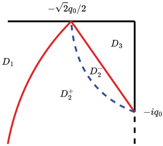
Figure 1. Four regions in k-complex plane.

Define $\xi ={\displaystyle \frac{x}{t}}$, $v_0=-4\sqrt{2}{q}_0$ and $v_1=4\sqrt{2}{q}_0$.

Theorem 1.

When there is a continuous spectrum and a second-order discrete spectrum $p\in D_1$, there exists a

$$v_s\left(p\right)=2\left[\mathrm{Re}\left(p\right)+{\displaystyle \frac{\mathrm{Re}\left[\lambda \right(p\left)\right]Im\left(p\right)}{Im\left[\lambda \right(p\left)\right]}}\right]\in (-\infty ,v_0).$$

(5)

The asymptotic behavior is as follows.

1.

When $\xi <v_s$, $q(x,t)\sim q_{-}{e}^{2i{g}_{\infty }\left(\xi \right)},$ where $g_{\infty }\left(\xi \right)$ is a real number defined by (85).

2.

When $v_s<\xi <v_0$, $q(x,t)\sim q_{-}{e}^{2i[g_{\infty }\left(\xi \right)+{\tilde{g}}_{\infty }]},$ where ${\tilde{g}}_{\infty }=4\arg [p+\lambda \left(p\right)]$, arg denotes the phase angle.

3.

When $v_0<\xi <0$,

$$q(x,t)\sim {\displaystyle \frac{q_0(q_0+{\alpha }_{im})}{q_{-}^{*}}}{\displaystyle \frac{\mathsf{\Theta }\left(\frac{\sqrt{q_0{\alpha }_{im}}}{mK\left(m\right)}(x-2{\alpha }_{\mathrm{Re}}t)-X_0+2v_{\infty }-\frac{1}{2}-\frac{\tilde{\omega }}{2\pi }\right)\mathsf{\Theta }\left(\frac{1}{2}\right)}{\mathsf{\Theta }\left(\frac{\sqrt{q_0{\alpha }_{im}}}{mK\left(m\right)}(x-2{\alpha }_{\mathrm{Re}}t)-X_0-\frac{1}{2}-\frac{\tilde{\omega }}{2\pi }\right)\mathsf{\Theta }(2v_{\infty }-\frac{1}{2})}}{e}^{2i\left[{\tilde{g}}_{\infty }+{\widehat{g}}_{\infty }\left(\xi \right)-G_{\infty }\left(\xi \right)t\right]},$$

(6)

where Θ is defined by (163), ${\alpha }_{\mathrm{Re}},{\alpha }_{im}$ and m are defined by (131), and $K\left(m\right)$ is the complete elliptic integral of the first kind. ${\tilde{g}}_{\infty }=4\arg \left[p+\lambda \left(p\right)\right]$, $v_{\infty },\tilde{\omega },{\widehat{g}}_{\infty },X_0$ and $G_{\infty }$ are functions of $\xi ={\displaystyle \frac{x}{t}}$ and respectively defined by (165), (154), (147), (169) and (136).

4.

When $0<\xi <v_1$,

$$q(x,t)\sim {\displaystyle \frac{q_0(q_0+{\alpha }_{im})}{q_{+}^{*}}}{\displaystyle \frac{\mathsf{\Theta }\left(\frac{\sqrt{q_0{\alpha }_{im}}}{mK\left(m\right)}(x-2{\alpha }_{\mathrm{Re}}t)-X_0+2v_{\infty }-\frac{1}{2}-\frac{\tilde{\omega }}{2\pi }\right)\mathsf{\Theta }\left(\frac{1}{2}\right)}{\mathsf{\Theta }\left(\frac{\sqrt{q_0{\alpha }_{im}}}{mK\left(m\right)}(x-2{\alpha }_{\mathrm{Re}}t)-X_0-\frac{1}{2}-\frac{\tilde{\omega }}{2\pi }\right)\mathsf{\Theta }(2v_{\infty }-\frac{1}{2})}}{e}^{2i\left[{\tilde{g}}_{\infty }+{\widehat{g}}_{\infty }\left(\xi \right)-G_{\infty }\left(\xi \right)t\right]}.$$

(7)

5.

When $\xi >v_1$, $q(x,t)\sim q_{+}{e}^{2i[g_{\infty }\left(\xi \right)+{\tilde{g}}_{\infty }]}$.

It is noted that when there is no continuous spectrum, $v_s$ represents the propagation speed of the solitary wave corresponding to the second-order discrete spectrum in an asymptotic sense. In Theorem 1, $\xi <v_s$ describes the asymptotic behavior of the solution to the left of the solitary wave and $\xi >v_s$ describes that to the right of the solitary wave.

Theorem 2.

When there is a continuous spectrum and a second-order discrete spectrum $p\in D_2$, there exists ${\tilde{v}}_s\left(p\right)\in (v_s\left(p\right),0)$ defined by $\mathrm{Re}\left[ih({\tilde{v}}_s,p)\right]=0$. Here $h(\xi ,k)$is defined by (132). The asymptotic behavior is as follows.

1.

When $\xi <v_0$, $q(x,t)\sim q_{-}{e}^{2i{g}_{\infty }\left(\xi \right)}.$

2.

When $v_0<\xi <{\tilde{v}}_s$,

$$q(x,t)\sim {\displaystyle \frac{q_0(q_0+{\alpha }_{im})}{q_{-}^{*}}}{\displaystyle \frac{\mathsf{\Theta }\left(\frac{\sqrt{q_0{\alpha }_{im}}}{mK\left(m\right)}(x-2{\alpha }_{\mathrm{Re}}t)-X_0+2v_{\infty }-\frac{1}{2}\right)\mathsf{\Theta }\left(\frac{1}{2}\right)}{\mathsf{\Theta }\left(\frac{\sqrt{q_0{\alpha }_{im}}}{mK\left(m\right)}(x-2{\alpha }_{\mathrm{Re}}t)-X_0-\frac{1}{2}\right)\mathsf{\Theta }(2v_{\infty }-\frac{1}{2})}}{e}^{2i\left[{\widehat{g}}_{\infty }\left(\xi \right)-G_{\infty }\left(\xi \right)t\right]}.$$

(8)

3.

When ${\tilde{v}}_s<\xi <0$,

$$q(x,t)\sim {\displaystyle \frac{q_0(q_0+{\alpha }_{im})}{q_{-}^{*}}}{\displaystyle \frac{\mathsf{\Theta }\left(\frac{\sqrt{q_0{\alpha }_{im}}}{mK\left(m\right)}(x-2{\alpha }_{\mathrm{Re}}t)-X_0+2v_{\infty }-\frac{1}{2}-\frac{\tilde{\omega }}{2\pi }\right)\mathsf{\Theta }\left(\frac{1}{2}\right)}{\mathsf{\Theta }\left(\frac{\sqrt{q_0{\alpha }_{im}}}{mK\left(m\right)}(x-2{\alpha }_{\mathrm{Re}}t)-X_0-\frac{1}{2}-\frac{\tilde{\omega }}{2\pi }\right)\mathsf{\Theta }(2v_{\infty }-\frac{1}{2})}}{e}^{2i\left[{\tilde{g}}_{\infty }+{\widehat{g}}_{\infty }\left(\xi \right)-G_{\infty }\left(\xi \right)t\right]}.$$

(9)

4.

When $0<\xi <v_1$,

$$q(x,t)\sim {\displaystyle \frac{q_0(q_0+{\alpha }_{im})}{q_{+}^{*}}}{\displaystyle \frac{\mathsf{\Theta }\left(\frac{\sqrt{q_0{\alpha }_{im}}}{mK\left(m\right)}(x-2{\alpha }_{\mathrm{Re}}t)-X_0+2v_{\infty }-\frac{1}{2}-\frac{\tilde{\omega }}{2\pi }\right)\mathsf{\Theta }\left(\frac{1}{2}\right)}{\mathsf{\Theta }\left(\frac{\sqrt{q_0{\alpha }_{im}}}{mK\left(m\right)}(x-2{\alpha }_{\mathrm{Re}}t)-X_0-\frac{1}{2}-\frac{\tilde{\omega }}{2\pi }\right)\mathsf{\Theta }(2v_{\infty }-\frac{1}{2})}}{e}^{2i\left[{\tilde{g}}_{\infty }+{\widehat{g}}_{\infty }\left(\xi \right)-G_{\infty }\left(\xi \right)t\right]}.$$

(10)

5.

When $\xi >v_1$, $q(x,t)\sim q_{+}{e}^{2i[g_{\infty }\left(\xi \right)+{\tilde{g}}_{\infty }]}$.

Theorem 2 uses ${\tilde{v}}_s$ as the dividing line to characterize the asymptotic behavior rather than $v_s$ in Theorem 1. That is, the solitary wave is influenced by the perturbation and changes the propagation speed ${\tilde{v}}_s$. Notice that it slows down, as ${\tilde{v}}_s>v_s$.

Now we explain Theorems 1 and 2 from the perspective of perturbations. To begin with, we briefly review the asymptotic behavior presented in [16] where only a perturbation corresponding to the continuous spectrum presents.

1.

When $\xi <0$, $q(x,t)\sim q_{-}{e}^{2i{g}_{\infty }\left(\xi \right)}.$

2.

When $v_0<\xi <0$,

$$q(x,t)\sim {\displaystyle \frac{q_0(q_0+{\alpha }_{im})}{q_{-}^{*}}}{\displaystyle \frac{\mathsf{\Theta }\left(\frac{\sqrt{q_0{\alpha }_{im}}}{mK\left(m\right)}(x-2{\alpha }_{\mathrm{Re}}t)-X_0+2v_{\infty }-\frac{1}{2}\right)\mathsf{\Theta }\left(\frac{1}{2}\right)}{\mathsf{\Theta }\left(\frac{\sqrt{q_0{\alpha }_{im}}}{mK\left(m\right)}(x-2{\alpha }_{\mathrm{Re}}t)-X_0-\frac{1}{2}\right)\mathsf{\Theta }(2v_{\infty }-\frac{1}{2})}}{e}^{2i\left[{\widehat{g}}_{\infty }\left(\xi \right)-G_{\infty }\left(\xi \right)t\right]}.$$

(11)

3.

When $0<\xi <v_1$,

$$q(x,t)\sim {\displaystyle \frac{q_0(q_0+{\alpha }_{im})}{q_{+}^{*}}}{\displaystyle \frac{\mathsf{\Theta }\left(\frac{\sqrt{q_0{\alpha }_{im}}}{mK\left(m\right)}(x-2{\alpha }_{\mathrm{Re}}t)-X_0+2v_{\infty }-\frac{1}{2}\right)\mathsf{\Theta }\left(\frac{1}{2}\right)}{\mathsf{\Theta }\left(\frac{\sqrt{q_0{\alpha }_{im}}}{mK\left(m\right)}(x-2{\alpha }_{\mathrm{Re}}t)-X_0-\frac{1}{2}\right)\mathsf{\Theta }(2v_{\infty }-\frac{1}{2})}}{e}^{2i\left[{\widehat{g}}_{\infty }\left(\xi \right)-G_{\infty }\left(\xi \right)t\right]}.$$

(12)

4.

When $\xi >v_1$, $q(x,t)\sim q_{+}{e}^{2i{g}_{\infty }\left(\xi \right)}$.

By comparison, it is evident that the presence of the second-order discrete spectrum has altered the perturbation in Theorems 1 and 2. We discuss the additional terms $\tilde{\omega }$ and ${\tilde{g}}_{\infty }$. On the one hand, ${\tilde{g}}_{\infty }$ causes a fixed phase shift $4\arg [p+\lambda (p\left)\right]$ in the perturbation. In contrast to this conclusion, the first-order soliton only induces a phase shift of $2\arg [p+\lambda (p\left)\right]$ [16]. On the other hand, $\tilde{\omega }$ affects the asymptotic behavior of the amplitude of $q(x,t)$. For the perturbation corresponding to the continuous spectrum, we have the following observation:

1.

When $\xi <v_0$, $\left|q(x,t)\right|=|q_{-}|=q_0.$

2.

When $v_0<\xi <v_1$,

$$\left|q(x,t)\right|={\left[{(q_0+{\alpha }_{im})}^2-4q_0{\alpha }_{im}{sn}^2(\sqrt{{\alpha }_{\mathrm{Re}}^2+{(q_0+{\alpha }_{im})}^2}(x-2{\alpha }_{\mathrm{Re}}t)-2K\left(m\right)X,m)\right]}^{{\displaystyle \frac{1}{2}}}.$$

(13)

3.

When $\xi >v_1$, $\left|q(x,t)\right|=|q_{+}|=q_0.$

From Theorem 1, as for $p\in D_1$, the modulus of $q(x,t)$ is as follows.

1.

When $\xi <v_0$, it holds that $\left|q(x,t)\right|=|q_{-}|=q_0.$

2.

When $v_0<\xi <v_1$, it holds that

$$\left|q(x,t)\right|={\left[{(q_0+{\alpha }_{im})}^2-4q_0{\alpha }_{im}{sn}^2(\sqrt{{\alpha }_{\mathrm{Re}}^2+{(q_0+{\alpha }_{im})}^2}(x-2{\alpha }_{\mathrm{Re}}t)-2K\left(m\right)X-{\displaystyle \frac{K\left(m\right)}{\pi }}\tilde{\omega },m)\right]}^{{\displaystyle \frac{1}{2}}},$$

(14)

where sn is the elliptic sine function.

3.

When $\xi >v_1$, $\left|q(x,t)\right|=|q_{+}|=q_0.$

Comparing (13) and (14), we observe that $\tilde{\omega }$ causes a change in the phase of the elliptic sine function. The presence of the second-order discrete spectrum leads to a spatial translation in the amplitude of the disturbance, but the overall shape remains unchanged.

From Theorem 2, when $p\in D_2^{+}$, the modulus of $q(x,t)$ is as follows.

1.

When $\xi <v_0$, $\left|q(x,t)\right|=|q_{-}|=q_0.$

2.

When $v_0<\xi <{\tilde{v}}_s$,

$$\left|q(x,t)\right|={\left[{(q_0+{\alpha }_{im})}^2-4q_0{\alpha }_{im}{sn}^2(\sqrt{{\alpha }_{\mathrm{Re}}^2+{(q_0+{\alpha }_{im})}^2}(x-2{\alpha }_{\mathrm{Re}}t)-2K\left(m\right)X,m)\right]}^{{\displaystyle \frac{1}{2}}},$$

(15)

3.

When ${\tilde{v}}_s<\xi <v_1$,

$$\left|q(x,t)\right|={\left[{(q_0+{\alpha }_{im})}^2-4q_0{\alpha }_{im}{sn}^2(\sqrt{{\alpha }_{\mathrm{Re}}^2+{(q_0+{\alpha }_{im})}^2}(x-2{\alpha }_{\mathrm{Re}}t)-2K\left(m\right)X-{\displaystyle \frac{K\left(m\right)}{\pi }}\tilde{\omega },m)\right]}^{{\displaystyle \frac{1}{2}}},$$

(16)

4.

When $\xi >v_1$, $\left|q(x,t)\right|=|q_{+}|=q_0.$

In this situation, for $\xi <{\tilde{v}}_s$, the amplitude of the disturbance remains unaffected. For $\xi >{\tilde{v}}_s$, the amplitude of the perturbation undergoes spatial translation.

The rest of this paper is organized as follows.

• Section 2: Introduction to the Riemann–Hilbert problem in the context of inverse scattering transform.
• Section 3: Analysis of the asymptotic behavior of the time terms in the jump conditions to determine the matrix factorization method used in the Deift–Zhou nonlinear steepest descent method.
• Section 4: Deformation of the Riemann–Hilbert problem and analysis of the main component of the solution to the deformed problem. These lead to the asymptotic behavior of the solution to the nonlinear Schrödinger equation, hence proves Theorems 1 and 2.
• Section 5: Numerical simulations to validate the results.

2. Riemann–Hilbert Problem

Consider the asymptotic scattering problem at infinity

$$\begin{array}{cc}\hfill {\phi }_x& =X_{\pm }\phi ,\hfill \\ \hfill {\phi }_t& =T_{\pm }\phi ,\hfill \end{array}$$

(17)

where $X_{\pm }=ik{P}_3+Q_{\pm },T_{\pm }=-2i{k}^2{P}_3-2k{Q}_{\pm },Q_{\pm }=\left(\begin{array}{cc}0& q_{\pm }\\ -q_{\pm }^{*}& 0\end{array}\right).$ The eigenvalues of $X_{\pm }$ are $\pm i\lambda$, where

$${\lambda }^2=k^2+q_0^2.$$

(18)

The multi-valued function $\lambda \left(k\right)$ in the k-complex plane takes $\pm iq$ as branch points. We map the Riemann surface $\left\{(k,\lambda )|{\lambda }^2=k^2+q_0^2\right\}$ onto the first sheet of the complex plane and take one single-valued branch $\lambda \left(k\right)=\sqrt{k^2+q_0^2}$. As shown in Figure 2, we introduce a branch cut $B=i[-q_0,q_0]$ which is oriented from $k=-i{q}_0$ to $k=i{q}_0$. Denote $B=B^{+}\cup B^{-}$, where $B^{+}=i[0,q_0]$ and $B^{-}=i[-q_0,0]$. Then $\lambda \left(k\right)$ is a single-valued holomorphic function on $\mathbb{C}\setminus B$, with a discontinuity on B.

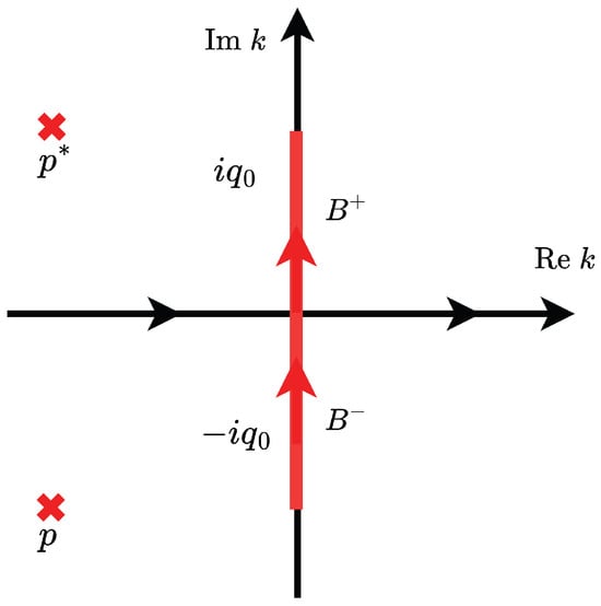
Figure 2. The branch cut $B=B^{+}+B^{-}$ and the pair of second-order discrete spectra p and $p^{*}$. The orientation of the limit is characterized by the arrow’s direction. The left limit of the function is defined as the limit acquired when the function approaches the oriented curve from its left orientation, while the right limit corresponds to its right orientation.

Thus, defining $\lambda \left(k\right)$ as its right limit ${\lambda }^{-}\left(k\right)$ on B, we get

$$\lambda \left(k\right)=\left\{\begin{array}{c}\sqrt{k^2+q_0^2}, k\in {\mathbb{R}}^{+}\cup B,\\ -\sqrt{k^2+q_0^2}, k\in {\mathbb{R}}^{-}.\end{array}\right.$$

(19)

This gives ${\lambda }^{+}\left(k\right)=-\lambda \left(k\right)$, where ${\lambda }^{+}\left(k\right)$ denotes the left limit of $\lambda \left(k\right)$ on B. Thus, the eigenvector matrix corresponding to the eigenvalues $\pm i\lambda \left(k\right)$ is

$$E_{\pm }\left(k\right)=\left(\begin{array}{cc}1& {\displaystyle \frac{i\left(\lambda \right(k)-k)}{q_{\pm }^{*}}}\\ {\displaystyle \frac{i\left(\lambda \right(k)-k)}{q_{\pm }}}& 1\end{array}\right).$$

(20)

We denote

$$d\left(k\right)=det{E}_{\pm }={\displaystyle \frac{2\lambda \left(k\right)}{\lambda \left(k\right)+k}}.$$

(21)

Because $T_{\pm }=-2k{X}_{\pm }$, the solution of (17) is

$$\phi =E_{\pm }{e}^{i\lambda (x-2kt)}C,$$

(22)

where C is a second order column vector. For $k\in \mathbb{R}\cup B$, define the Jost solutions ${\mathsf{\Psi }}_{\pm }(x,t,k)$, namely, the simultaneous solutions as $x\to \pm \infty$:

$${\mathsf{\Psi }}_{\pm }(x,t,k)=E_{\pm }\left(k\right)e^{i\theta (x,t,k)t{P}_3}+o\left(1\right), x\to \pm \infty ,$$

(23)

where $\theta (x,t,k)=\lambda \left(k\right)({\displaystyle \frac{x}{t}}-2k)$. Next, modify the Jost solutions (23) by

$${\widehat{\mu }}_{\pm }(x,t,k)={\mathsf{\Psi }}_{\pm }(x,t,k)e^{-i\theta (x,t,k)t{P}_3}=({\widehat{\mu }}_{\pm ,1},{\widehat{\mu }}_{\pm ,2}),$$

(24)

where ${\widehat{\mu }}_{\pm ,1},{\widehat{\mu }}_{\pm ,2}$ are column vectors. Substituting the modified Jost solutions into (3) gives the Volterra integral equation satisfied by the Jost solutions:

$$\begin{array}{cc}\hfill {\widehat{\mu }}_{-}(x,t,k)& =E_{-}+{\int }_{\infty }^x{E}_{-}{e}^{i\lambda (x-y)P_3}{E}_{-}^{-1}(Q(y,t)-Q_{-}){\widehat{\mu }}_{-}(x,t,k)e^{-i\lambda (x-y)P_3}dy,\hfill \\ \hfill {\widehat{\mu }}_{+}(x,t,k)& =E_{+}-{\int }_x^{\infty }{E}_{+}{e}^{i\lambda (x-y)P_3}{E}_{+}^{-1}(Q(y,t)-Q_{+}){\widehat{\mu }}_{+}(x,t,k)e^{-i\lambda (x-y)P_3}dy.\hfill \end{array}$$

(25)

The existence and analyticity of the modified Jost solutions can be proved by Neumann series [19]: for $k\in {\mathbb{R}}^{+}\cup B$, $Im\lambda \left(k\right)=0$, the modified Jost solutions exist and are unique. For $k\in {\mathbb{C}}^{+}\setminus B^{+}$, where ${\mathbb{C}}^{+}=\left\{k|Imk>0\right\}$, $Im\lambda \left(k\right)>0$, ${\widehat{\mu }}_{+,1}$ and ${\widehat{\mu }}_{-,2}$ can be analytically extended to $k\in {\mathbb{C}}^{+}\setminus B^{+}$ from $\mathbb{R}\cup B$. For $k\in {\mathbb{C}}^{-}\setminus B^{-}$, where ${\mathbb{C}}^{-}=\left\{k|Imk<0\right\}$, $Im\lambda \left(k\right)<0$, ${\widehat{\mu }}_{-,1}$ and ${\widehat{\mu }}_{+,2}$ can be analytically extended to $k\in {\mathbb{C}}^{-}\setminus B^{-}$ from $\mathbb{R}\cup B$.

If and only if $k\in {\mathbb{R}}^{+}\cup B$, both ${\widehat{\mu }}_{\pm }(x,t,k)$ exist. So $k\in {\mathbb{R}}^{+}\cup B$ is the continuous spectrum of the inverse scattering transform.

Both ${\mathsf{\Psi }}_{\pm }(x,t,k)$ are solutions of (3), so there exists a scattering matrix $S\left(k\right)$,

$$\forall k\in \mathbb{R}\cup B,\hspace{1em}{\mathsf{\Psi }}_{-}(x,t,k)={\mathsf{\Psi }}_{+}(x,t,k)S\left(k\right).$$

(26)

Here

$$S\left(k\right)=\left(\begin{array}{cc}a\left(k\right)& -b^{*}\left(k^{*}\right)\\ b\left(k\right)& a^{*}\left(k^{*}\right)\end{array}\right).$$

(27)

We denote $\overline{a}\left(k\right)=a^{*}\left(k^{*}\right)$ and $\overline{b}\left(k\right)=b^{*}\left(k^{*}\right)$ then

$$\begin{array}{c}\hfill a\left(k\right)={\displaystyle \frac{det({\mathsf{\Psi }}_{-,1},{\mathsf{\Psi }}_{+,2})}{d\left(k\right)}}, \overline{a}\left(k\right)={\displaystyle \frac{det({\mathsf{\Psi }}_{+,1},{\mathsf{\Psi }}_{-,2})}{d\left(k\right)}},\end{array}$$

(28a)

$$\begin{array}{c}\hfill b\left(k\right)={\displaystyle \frac{det({\mathsf{\Psi }}_{+,1},{\mathsf{\Psi }}_{-,1})}{d\left(k\right)}}, \overline{b}\left(k\right)={\displaystyle \frac{det({\mathsf{\Psi }}_{+,2},{\mathsf{\Psi }}_{-,2})}{d\left(k\right)}},\end{array}$$

(28b)

In this way, $a\left(k\right)$ is analytically extended to ${\mathbb{C}}^{-}\setminus B^{-}$.

In the following discussions, with a little abuse of notation, we denote the right limit of $\lambda \left(k\right)$ on B still as $\lambda \left(k\right)$. Biondini [16] proposed the jump condition of the modified Jost solutions

$$\begin{array}{cc}\hfill \forall k\in B^{-}, {\widehat{\mu }}_{-,1}^{+}(x,t,k)& ={\displaystyle \frac{\lambda +k}{i{q}_{-}}}{\widehat{\mu }}_{-,2}(x,t,k),\hfill \\ \hfill \forall k\in B^{-}, {\widehat{\mu }}_{+,2}^{+}(x,t,k)& ={\displaystyle \frac{\lambda +k}{i{q}_{+}^{*}}}{\widehat{\mu }}_{+,1}(x,t,k),\hfill \\ \hfill \forall k\in B^{+}, {\widehat{\mu }}_{-,2}^{+}(x,t,k)& ={\displaystyle \frac{\lambda +k}{i{q}_{-}^{*}}}{\widehat{\mu }}_{-,1}(x,t,k),\hfill \\ \hfill \forall k\in B^{+}, {\widehat{\mu }}_{+,1}^{+}(x,t,k)& ={\displaystyle \frac{\lambda +k}{i{q}_{+}}}{\widehat{\mu }}_{+,2}(x,t,k).\hfill \end{array}$$

(29)

The jump condition of the scatteing matrix coefficient a is

$$\forall k\in B^{-}, {\overline{a}}^{+}\left(k\right)={\displaystyle \frac{q_{-}}{q_{+}}}a\left(k\right).$$

(30)

Up to this point, the jump conditions required for the Riemann–Hilbert problem are given. Thus, we introduce a piecewise meromorphic function

$$M(x,t,k)=\left\{\begin{array}{c}\left({\displaystyle \frac{{\widehat{\mu }}_{+,1}(x,t,k)}{\overline{a}\left(k\right)d\left(k\right)}}, {\widehat{\mu }}_{-,2}(x,t,k)\right), k\in {\mathbb{C}}^{+}\setminus B^{+},\\ \left({\widehat{\mu }}_{-,1}(x,t,k), {\displaystyle \frac{{\widehat{\mu }}_{+,2}(x,t,k)}{a\left(k\right)d\left(k\right)}}\right), k\in {\mathbb{C}}^{-}\setminus B^{-}.\end{array}\right.$$

(31)

According to (24) and (28a), we know when $k\in {\mathbb{C}}^{+}\setminus B^{+}$,

$$detM=det\left\{\left({\displaystyle \frac{{\widehat{\mu }}_{+,1}(x,t,k)}{\overline{a}\left(k\right)d\left(k\right)}}, {\widehat{\mu }}_{-,2}(x,t,k)\right)\right\}={\displaystyle \frac{1}{\overline{a}\left(k\right)d\left(k\right)}}det({\mathsf{\Psi }}_{+,1},{\mathsf{\Psi }}_{-,2})=1.$$

(32)

Similar analysis applied to the case $k\in {\mathbb{C}}^{-}\setminus B^{-}$ shows $detM=1$. Define the reflection coefficient $r\left(k\right)=-{\displaystyle \frac{b\left(k\right)}{\overline{a}\left(k\right)}}$, the jump condition of $M(x,t,k),\forall k\in \mathbb{R}$ is given as

$$\forall k\in \mathbb{R},M^{+}(x,t,k)=M^{-}(x,t,k)\left(\begin{array}{cc}{\displaystyle \frac{1}{d\left(k\right)}}[1+r\left(k\right)\overline{r}\left(k\right)]& \overline{r}\left(k\right)e^{2i\theta (x,t,k)t}\\ r\left(k\right)e^{-2i\theta (x,t,k)t}& d\left(k\right)\end{array}\right).$$

(33)

Meanwhile, the jump condition for $k\in B$ is given by the jump conditions of the modified Jost solutions (29) and that of the scattering matrix coefficient (30), namely,

$$\begin{array}{cc}\hfill \forall k\in B^{+}, M^{+}(x,t,k)& =M^{-}(x,t,k)\left(\begin{array}{cc}-{\displaystyle \frac{\lambda \left(k\right)-k}{i{q}_{-}}}\overline{r}\left(k\right)e^{2i\theta (x,t,k)t}& {\displaystyle \frac{2\lambda \left(k\right)}{i{q}_{-}^{*}}}\\ {\displaystyle \frac{q_{-}^{*}}{2i\lambda \left(k\right)}}[1+r\left(k\right)\overline{r}\left(k\right)]& -{\displaystyle \frac{\lambda \left(k\right)+k}{i{q}_{-}^{*}}}r\left(k\right)e^{-2i\theta (x,t,k)t}\end{array}\right),\hfill \\ \hfill \forall k\in B^{-}, M^{+}(x,t,k)& =M^{-}(x,t,k)\left(\begin{array}{cc}{\displaystyle \frac{\lambda \left(k\right)+k}{i{q}_{-}}}\overline{r}\left(k\right)e^{2i\theta (x,t,k)t}& {\displaystyle \frac{q_{-}}{2i\lambda \left(k\right)}}[1+r\left(k\right)\overline{r}\left(k\right)]\\ {\displaystyle \frac{2\lambda \left(k\right)}{i{q}_{-}}} & {\displaystyle \frac{\lambda \left(k\right)-k}{i{q}_{-}^{*}}}r\left(k\right)e^{-2i\theta (x,t,k)t}\end{array}\right).\hfill \end{array}$$

(34)

In addition, we need to precise the asymptotic condition and series condition to analyze the Riemann–Hilbert problem. It is shown in [19] that the asymptotic condition of the Riemann–Hilbert problem is

$$\underset{k\to \infty }{lim}M(x,t,k)=I+O\left({\displaystyle \frac{1}{k}}\right).$$

(35)

The expansion of $M(x,t,k)$ at infinity shows that the solution of the nonlinear Schrödinger equation is obtained from

$$q(x,t)=\underset{k\to \infty }{lim}\left[-ik{M}_{1,2}(x,t,k)\right].$$

(36)

In ${\mathbb{C}}^{-}\setminus B^{-}$, ${\widehat{\mu }}_{-,1},{\widehat{\mu }}_{+,2},d\left(k\right)$ are analytic and $a\left(k\right)$ has a second-order zero at the discrete spectrum p, namely $a\left(p\right)=0, a^{\prime }\left(p\right)=0$. Performing Laurent expansion around $k=p$ as follows. In the following discussions, ′ denotes derivative with respect to k.

$$\begin{array}{cc}\hfill {\displaystyle \frac{{\widehat{\mu }}_{+,2}\left(k\right)}{a\left(k\right)d\left(k\right)}}& ={\displaystyle \frac{{\widehat{\mu }}_{+,2}\left(p\right)+{\widehat{\mu }}_{+,2}^{\prime }\left(p\right)(k-p)+{\widehat{\mu }}_{+,2}^{″}\left(p\right){(k-p)}^2/2+O\left({(k-p)}^3\right)}{[a^{″}\left(p\right){(k-p)}^2/2+a^{‴}\left(p\right){(k-p)}^3/6+O\left({(k-p)}^4\right)][d\left(p\right)+d^{\prime }\left(p\right)(k-p)+O\left({(k-p)}^2\right)]}}\hfill \\ \hfill & ={\displaystyle \frac{2{\widehat{\mu }}_{+,2}\left(p\right)}{a^{″}\left(p\right)d\left(p\right)}}{(k-p)}^{-2}+\left[{\displaystyle \frac{2{\widehat{\mu }}_{+,2}^{\prime }\left(p\right)}{a^{″}\left(p\right)d\left(p\right)}}-{\displaystyle \frac{2{\widehat{\mu }}_{+,2}\left(p\right)(a^{‴}\left(p\right)d\left(p\right)+3a^{″}\left(p\right)d^{\prime }\left(p\right))}{3{\left[a^{″}\left(p\right)\right]}^2}}\right]{(k-p)}^{-1}+O\left(1\right).\hfill \end{array}$$

(37)

Therefore the conditions of Laurent series are

$$\begin{array}{cc}\hfill \underset{k=p}{P_{-2}}\left[{\displaystyle \frac{{\widehat{\mu }}_{+,2}\left(k\right)}{a\left(k\right)d\left(k\right)}}\right]& ={\displaystyle \frac{2{\widehat{\mu }}_{+,2}\left(p\right)}{a^{″}\left(p\right)d\left(p\right)}},\hfill \\ \hfill \underset{k=p}{Res}\left[{\displaystyle \frac{{\widehat{\mu }}_{+,2}\left(k\right)}{a\left(k\right)d\left(k\right)}}\right]& =\left[{\displaystyle \frac{2{\widehat{\mu }}_{+,2}^{\prime }\left(p\right)}{a^{″}\left(p\right)d\left(p\right)}}-{\displaystyle \frac{2{\widehat{\mu }}_{+,2}\left(p\right)(a^{‴}\left(p\right)d\left(p\right)+3a^{″}\left(p\right)d^{\prime }\left(p\right))}{3{\left[a^{″}\left(p\right)\right]}^2}}\right],\hfill \end{array}$$

(38)

where $P_{-2}$ denotes the coefficient of the second term in the Laurent series. Consider $a\left(p\right)=0$, according to (28a), we have

$$det({\mathsf{\Psi }}_{-,1},{\mathsf{\Psi }}_{+,2})=0,$$

(39)

so there exists a constant $b_p$, making

$${\mathsf{\Psi }}_{+,2}(x,t,p)=b_p{\mathsf{\Psi }}_{-,1}(x,t,p).$$

(40)

Substituting (24) into (40), we have

$${\widehat{\mu }}_{+,2}(x,t,p)=b_p{e}^{2i\theta (x,t,p)t}{\widehat{\mu }}_{-,1}(x,t,p).$$

(41)

Substituting $a^{\prime }\left(p\right)=0$ into (28a), we have

$$0=a^{\prime }\left(p\right)={\left[{\displaystyle \frac{1}{d}}det({\mathsf{\Psi }}_{-,1}^{\prime },{\mathsf{\Psi }}_{+,2})+{\displaystyle \frac{1}{d}}det({\mathsf{\Psi }}_{-,1},{\mathsf{\Psi }}_{+,2}^{\prime })-{\displaystyle \frac{d^{\prime }}{d^2}}det({\mathsf{\Psi }}_{-,1},{\mathsf{\Psi }}_{+,2})\right]}_{k=p}.$$

(42)

Substituting (39) and (40) into (42), we have

$$det({\mathsf{\Psi }}_{-,1},{\mathsf{\Psi }}_{+,2}^{\prime }-b_p{\mathsf{\Psi }}_{-,1}^{\prime })=0.$$

(43)

So, there exists a constant $d_p$, making

$${\mathsf{\Psi }}_{+,2}^{\prime }=b_p{\mathsf{\Psi }}_{-,1}^{\prime }+d_p{\mathsf{\Psi }}_{-,1}.$$

(44)

Substituting (24) into (44), we find

$${\widehat{\mu }}_{+,2}^{\prime }=e^{2i\theta (x,t,p)t}\left[b_p{\widehat{\mu }}_{-,1}^{\prime }+(d_p+2i{\theta }^{\prime }{b}_{p}t){\widehat{\mu }}_{-,1}\right].$$

(45)

Substituting (41) and (45) into (38), we find

$$\begin{array}{cc}\hfill \underset{k=p}{P_{-2}}\left[{\displaystyle \frac{{\widehat{\mu }}_{+,2}\left(k\right)}{a\left(k\right)d\left(k\right)}}\right]& =A_p{e}^{2i\theta (x,t,p)t}{\widehat{\mu }}_{-,1},\hfill \\ \hfill \underset{k=p}{Res}\left[{\displaystyle \frac{{\widehat{\mu }}_{+,2}\left(k\right)}{a\left(k\right)d\left(k\right)}}\right]& =A_p{e}^{2i\theta (x,t,p)t}{\widehat{\mu }}_{-,1}^{\prime }+A_p{e}^{2i\theta (x,t,p)t}[B_p+2i{\theta }^{\prime }(x,t,p)t]{\widehat{\mu }}_{-,1},\hfill \end{array}$$

(46)

where

$$\begin{array}{c}\hfill A_p={\displaystyle \frac{2b_p}{a^{″}\left(p\right)d\left(p\right)}}, B_p={\displaystyle \frac{d_p}{b_p}}-{\displaystyle \frac{d\left(p\right)(a^{‴}\left(p\right)d\left(p\right)+3a^{″}\left(p\right)d^{\prime }\left(p\right))}{3a^{″}{\left(p\right)}^2}}.\end{array}$$

(47)

Thus, the series conditions of $M(x,t,k)$ at $k=p$ can be written as

$$\begin{array}{cc}\hfill \underset{k=p}{Res}M& =\left[0,\underset{k=p}{P_{-2}}\left({\displaystyle \frac{{\widehat{\mu }}_{+,2}\left(k\right)}{a\left(k\right)d\left(k\right)}}\right)\right]=M^{\prime }{N}_1+M{N}_2,\hfill \\ \hfill \underset{k=p}{P_{-2}}M& =\left[0,\underset{k=p}{Res}\left({\displaystyle \frac{{\widehat{\mu }}_{+,2}\left(k\right)}{a\left(k\right)d\left(k\right)}}\right)\right]=M{N}_1,\hfill \end{array}$$

(48)

where

$$\begin{array}{c}\hfill N_1=\left(\begin{array}{cc}0& A_p{e}^{2i\theta (x,t,p)t}\\ 0& 0\end{array}\right),\hspace{1em}{N}_2=\left(\begin{array}{cc}0& A_p{e}^{2i\theta (x,t,p)t}[B_p+2i{\theta }^{\prime }(x,t,p)t]\\ 0& 0\end{array}\right).\end{array}$$

(49)

The series conditions of $M(x,t,k)$ at $k=p^{*}$ then read

$$\begin{array}{cc}\hfill \underset{k=p^{*}}{Res}M& =\left[\underset{k=p^{*}}{P_{-2}}\left({\displaystyle \frac{{\widehat{\mu }}_{+,1}\left(k\right)}{\overline{a}\left(k\right)d\left(k\right)}}\right),0\right]=M^{\prime }{\widehat{N}}_1+M{\widehat{N}}_2,\hfill \\ \hfill \underset{k=p^{*}}{P_{-2}}M& =\left[\underset{k=p^{*}}{Res}\left({\displaystyle \frac{{\widehat{\mu }}_{+,1}\left(k\right)}{\overline{a}\left(k\right)d\left(k\right)}}\right),0\right]=M{\widehat{N}}_1,\hfill \end{array}$$

(50)

where

$$\begin{array}{c}\hfill {\widehat{A}}_p=-{\displaystyle \frac{2b_p^{*}}{{\overline{a}}^{″}{d}^{*}\left(p\right)}}, {\widehat{B}}_p={\displaystyle \frac{d_p^{*}}{b_p^{*}}}-{\displaystyle \frac{d^{*}({\overline{a}}^{‴}\left(p\right)d^{*}\left(p\right)+3{\overline{a}}^{″}\left(p\right){\left(d^{\prime }\left(p\right)\right)}^{*})}{3{\overline{a}}^{″}{\left(p\right)}^2}},\end{array}$$

(51)

$$\begin{array}{c}\hfill {\widehat{N}}_1=\left(\begin{array}{cc}0& 0\\ {\widehat{A}}_p{e}^{-2i\theta (x,t,p^{*})t}& 0\end{array}\right),\hspace{1em}{\widehat{N}}_2=\left(\begin{array}{cc}0& 0\\ {\widehat{A}}_p{e}^{-2i\theta (x,t,p^{*})t}[{\widehat{B}}_p-2i{\theta }^{\prime }(x,t,p^{*})t]& 0\end{array}\right).\end{array}$$

(52)

In conclusion, we have jump conditions of the piecewise meromorphic function $M(x,t,k)$, the asymptotic condition (35), and the series conditions (48) and (50).

3. The Asymptotic Behavior of the Time Terms

In this section, we study the asymptotic behavior of the time terms for the Riemann–Hilbert problem. The exponential terms $e^{\pm 2i\theta (x,t,k)t}$ appear in the jump conditions (33), (34) and the series conditions (48)–(52). We investigate the asymptotic behavior on the line $x=\xi t$ with a fixed slope $\xi$ in $(x,t)$ plane. In this case,

$$\theta (x,t,k)=\lambda \left(k\right)\left({\displaystyle \frac{x}{t}}-2k\right)=\lambda \left(k\right)(\xi -2k).$$

(53)

We write $\theta (x,t,k)$ as $\theta (\xi ,k)$ without making confusion. To use the Deift–Zhou steepest descent method for analyzing the asymptotic behavior, we consider the sign structure of

$$\mathrm{Re}\left[i\theta (\xi ,k)\right]=-Im\left[\lambda \left(k\right)\right][\xi -2\mathrm{Re}\left(k\right)]+2\mathrm{Re}\left[\lambda \left(k\right)\right]Im\left(k\right),$$

(54)

which is depicted in Figure 3.

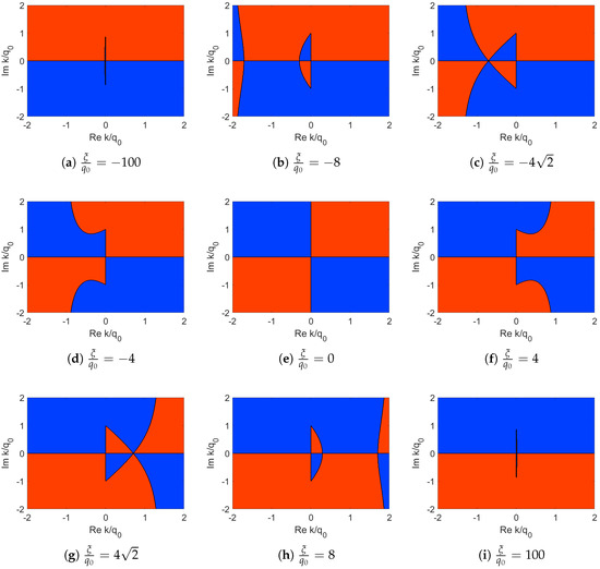
Figure 3. Sign of $\mathrm{Re}\left[i\theta (\xi ,k)\right]$ as $\xi$ increases from $-\infty$ to $+\infty$. Red: $\mathrm{Re}\left[i\theta (\xi ,k)\right]>0$, Blue: $\mathrm{Re}\left[i\theta (\xi ,k)\right]<0$.

Considering the symmetry of $\xi$, we only need to study the sign structure of $\mathrm{Re}\left[i\theta (\xi ,k)\right]$ for $\xi <0$. Denote $v_0=-4\sqrt{2}{q}_0$ and $v_1=4\sqrt{2}{q}_0$. When $\xi <v_0$, the curve $\mathrm{Re}\left[i\theta (\xi ,k)\right]=0$ intersects $Im\left(k\right)=0$ at two points

$$\begin{array}{cc}\hfill k_1\left(\xi \right)& ={\displaystyle \frac{\xi -\sqrt{{\xi }^2-v_0^2}}{8}},\hfill \\ \hfill k_2\left(\xi \right)& ={\displaystyle \frac{\xi +\sqrt{{\xi }^2-v_0^2}}{8}},\hfill \end{array}$$

(55)

where $k_1\left(\xi \right)$ is to the left of $k_2\left(\xi \right)$. When $\xi =v_0$, the curve $\mathrm{Re}\left[i\theta (\xi ,k)\right]=0$ intersects $Im\left(k\right)=0$ at one point $k=-{\displaystyle \frac{\sqrt{2}{q}_0}{2}}$. When $v_0<\xi <0$, the curve $\mathrm{Re}\left[i\theta (\xi ,k)\right]=0$ has no intersection with $Im\left(k\right)=0$, and is directly connected to B.

4. Proof of Theorem 1

Consider $p\in D_1$. As Figure 1 shows, the right boundary of $D_1$ is the curve $\mathrm{Re}\left[i\theta (v_0,k)\right]=0$. So, there exists a value $v_s$ of $\xi$, such that the curve $\mathrm{Re}\left[i\theta (v_s,k)\right]=0$ goes right through the discrete spectrum, namely $\mathrm{Re}\left[i\theta (v_s,p)\right]=\mathrm{Re}\left[i\theta (v_s,p^{*})\right]=0$. Substituting it into (54), we have

$$v_s=2\left[\mathrm{Re}\left(p\right)+{\displaystyle \frac{\mathrm{Re}\left(\lambda \right(p\left)\right)}{Im\left(\lambda \right(p\left)\right)}}Im\left(p\right)\right].$$

(56)

Here $v_s\left(p\right)$ is the asymptotic propagation speed of the solitary wave solution corresponding to the second-order discrete spectrum. Next, following [18], we divide $(-\infty ,0)$ into three intervals $(\infty ,v_s)$, $(v_s,v_0)$ and $(v_0,0)$, and analyze the asymptotic behavior under these three conditions separately.

4.1. $\xi \in (-\infty ,v_s)$

When $\xi <v_s$, p is to the right of $\mathrm{Re}\left[i\theta (v_0,k)\right]=0$. The two intersection points $k_1\left(\xi \right)$ and $k_2\left(\xi \right)$, as (55) shows, are between $\mathrm{Re}\left[i\theta (v_0,k)\right]=0$ and the real axis. Although there is a sign change near $k_2$, as shown in Figure 3, it only occurs in the small region from $k_2\left(\xi \right)$ to B. Therefore, we only decompose the jump matrix differently near $k_1$ and ensure that the jump curve crosses this small region in subsequent transformations, which does not affect the decomposition terms of the time component on the curve.

The jump matrix in the jump condition on $\mathbb{R}$ is decomposed as

$$\left(\begin{array}{cc}{\displaystyle \frac{1}{d\left(k\right)}}[1+r\left(k\right)\overline{r}\left(k\right)]& \overline{r}\left(k\right)e^{2i\theta (x,t,k)t}\\ r\left(k\right)e^{-2i\theta (x,t,k)t}& d\left(k\right)\end{array}\right)=\left\{\begin{array}{c}{V}_2^{\left(1\right)}{V}_0^{\left(1\right)}{V}_1^{\left(1\right)}, \mathrm{Re}\left(k\right)<k_1,\\ V_3^{\left(1\right)}{V}_4^{\left(1\right)}, \mathrm{Re}\left(k\right)>k_1,\end{array}\right.$$

(57)

where

$$\begin{array}{c}\hfill V_0^{\left(1\right)}=\left(\begin{array}{cc}1+r\overline{r}& 0\\ 0& {\displaystyle \frac{1}{1+r\overline{r}}}\end{array}\right), V_1^{\left(1\right)}=\left(\begin{array}{cc}{d}^{-{\displaystyle \frac{1}{2}}}& {\displaystyle \frac{d^{\frac{1}{2}}\overline{r}{e}^{2i\theta t}}{1+r\overline{r}}}\\ 0& d^{{\displaystyle \frac{1}{2}}}\end{array}\right), V_2^{\left(1\right)}=\left(\begin{array}{cc}{d}^{-{\displaystyle \frac{1}{2}}}& 0\\ {\displaystyle \frac{d^{\frac{1}{2}}r{e}^{-2i\theta t}}{1+r\overline{r}}}& d^{{\displaystyle \frac{1}{2}}}\end{array}\right),\\ \hfill V_3^{\left(1\right)}=\left(\begin{array}{cc}{d}^{-{\displaystyle \frac{1}{2}}}& 0\\ d^{{\displaystyle \frac{1}{2}}}r{e}^{-2i\theta t}& d^{{\displaystyle \frac{1}{2}}}\end{array}\right), V_4^{\left(1\right)}=\left(\begin{array}{cc}{d}^{-{\displaystyle \frac{1}{2}}}& d^{{\displaystyle \frac{1}{2}}}\overline{r}{e}^{2i\theta t}\\ 0& d^{{\displaystyle \frac{1}{2}}}\end{array}\right).\end{array}$$

(58)

The jump matrices in the jump condition on B are decomposed as

$$\begin{array}{ccc}\hfill & \forall k\in B^{+}, \left(\begin{array}{cc}-{\displaystyle \frac{\lambda \left(k\right)-k}{i{q}_{-}}}\overline{r}\left(k\right)e^{2i\theta (\xi ,k)t}& {\displaystyle \frac{2\lambda \left(k\right)}{i{q}_{-}^{*}}}\\ {\displaystyle \frac{q_{-}^{*}}{2i\lambda \left(k\right)}}[1+r\left(k\right)\overline{r}\left(k\right)]& -{\displaystyle \frac{\lambda \left(k\right)+k}{i{q}_{-}^{*}}}r\left(k\right)e^{-2i\theta (\xi ,k)t}\end{array}\right)\hfill & \hfill ={\left(V_3^{\left(1\right)-}\right)}^{-1}{V}_B{\left(V_3^{\left(1\right)}\right)}^{+},\\ \hfill & \forall k\in B^{-}, \left(\begin{array}{cc}{\displaystyle \frac{\lambda \left(k\right)+k}{i{q}_{-}}}\overline{r}\left(k\right)e^{2i\theta (\xi ,k)t}& {\displaystyle \frac{q_{-}}{2i\lambda \left(k\right)}}[1+r\left(k\right)\overline{r}\left(k\right)]\\ {\displaystyle \frac{2\lambda \left(k\right)}{i{q}_{-}}} & {\displaystyle \frac{\lambda \left(k\right)-k}{i{q}_{-}^{*}}}r\left(k\right)e^{-2i\theta (\xi ,k)t}\end{array}\right)\hfill & \hfill ={\left(V_4^{\left(1\right)-}\right)}^{-1}{V}_B{\left(V_4^{\left(1\right)}\right)}^{+},\end{array}$$

(59)

where $V_3^{\left(1\right)\pm }$ is the left and right limit of $V_3$, and $V_4^{\left(1\right)\pm }$ are those of $V_4$. Moreover, $V_B$ is a constant matrix

$$V_B=\left(\begin{array}{cc}0& {\displaystyle \frac{q_{-}}{i{q}_0}}\\ {\displaystyle \frac{q_{-}^{*}}{i{q}_0}}& 0\end{array}\right).$$

(60)

First Deformation. Define the function matrix $M^{\left(1\right)}(x,t,k)$ as shown in Figure 4a. The dashed line represents $\mathrm{Re}\left[i\theta (v_0,k)\right]=0$. Since the jump matrices of $L_{3,1}$ and $L_{3,2}$ are the same, if two curves extend a small portion very close to the origin, the jump changes of the two curves cancel in this small segment, making the function still continuous. This is equivalent to splicing the two curves together. Next, we adjust the values in each region. The adjustment enables the curves formed by $L_{3,1}$ and $L_{3,2}$ to continue extending outward until they no longer include the region where the sign change occurs from $k_2$ to B. Similarly, we splice $L_{3,3}$ and $L_{3,4}$ as shown in Figure 4b and Figure 5a. As depicted in Figure 5b, continue using curves with the same jump matrices at both endpoints of B to cancel jumps and move the curve upward, combining $L_{3,2}$ and $L_{3,3}$. Eventually, we obtain a curve $L_3$ that starts from $k_1$, bypasses B, and goes to infinity on the right. Similarly $L_4$ is obtained in the lower half-plane. The values of the region after the first deformation are shown in Figure 5c.

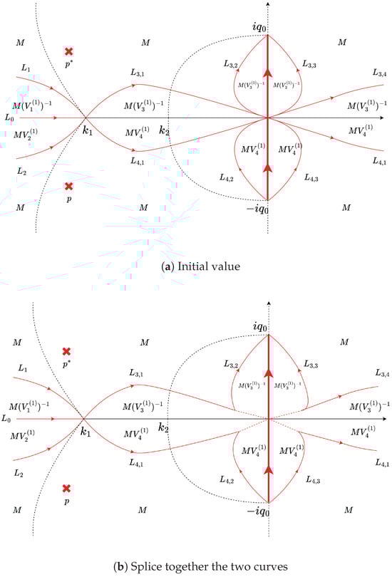
Figure 4. Diagram of the first deformation 1, substep 1. redHere the dashed lines denote the curve $\mathrm{Re}\left[i\theta (\xi ,k)\right]=0$.

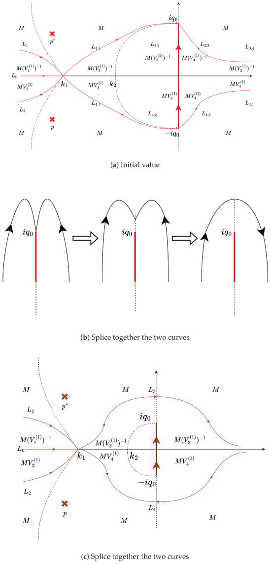
Figure 5. Diagram of the first deformation, substep 2.

The jump conditions are

$$\begin{array}{cc}\hfill \forall k\in L_j, M^{\left(1\right)+}=& M^{\left(1\right)-}{V}_j^{\left(1\right)}, j=0,\dots ,4,\hfill \\ \hfill \forall k\in B, M^{\left(1\right)+}=& M^{\left(1\right)-}{V}_B^{\left(1\right)},\hfill \end{array}$$

(61)

where

$$\begin{array}{c}\hfill V_B^{\left(1\right)}=\left(\begin{array}{cc}0& {\displaystyle \frac{q_{-}}{i{q}_0}}\\ {\displaystyle \frac{q_{-}^{*}}{i{q}_0}}& 0\end{array}\right), V_0^{\left(1\right)}=\left(\begin{array}{cc}1+r\overline{r}& 0\\ 0& {\displaystyle \frac{1}{1+r\overline{r}}}\end{array}\right), V_1^{\left(1\right)}=\left(\begin{array}{cc}{d}^{-{\displaystyle \frac{1}{2}}}& {\displaystyle \frac{d^{\frac{1}{2}}\overline{r}{e}^{2i\theta t}}{1+r\overline{r}}}\\ 0& d^{{\displaystyle \frac{1}{2}}}\end{array}\right),\\ \hfill V_2^{\left(1\right)}=\left(\begin{array}{cc}{d}^{-{\displaystyle \frac{1}{2}}}& 0\\ {\displaystyle \frac{d^{\frac{1}{2}}r{e}^{-2i\theta t}}{1+r\overline{r}}}& d^{{\displaystyle \frac{1}{2}}}\end{array}\right), V_3^{\left(1\right)}=\left(\begin{array}{cc}{d}^{-{\displaystyle \frac{1}{2}}}& 0\\ d^{-{\displaystyle \frac{1}{2}}}r{e}^{-2i\theta t}& d^{{\displaystyle \frac{1}{2}}}\end{array}\right), V_4^{\left(1\right)}=\left(\begin{array}{cc}{d}^{-{\displaystyle \frac{1}{2}}}& d^{-{\displaystyle \frac{1}{2}}}\overline{r}{e}^{2i\theta t}\\ 0& d^{{\displaystyle \frac{1}{2}}}\end{array}\right).\end{array}$$

(62)

The function value at p and $p^{*}$ remains unchanged, so the series conditions for the nth deformation are written formally as

$$\begin{array}{cc}\hfill \underset{k=p}{P_{-2}}{M}^{\left(n\right)}& =M^{\left(n\right)}{N}_1^{\left(n\right)}, \underset{k=p}{Res}{M}^{\left(n\right)}={\left(M^{\left(n\right)}\right)}^{\prime }{N}_1^{\left(n\right)}+M^{\left(n\right)}{N}_2^{\left(n\right)},\hfill \\ \hfill \underset{k=p^{*}}{P_{-2}}{M}^{\left(n\right)}& =M^{\left(n\right)}{\widehat{N}}_1^{\left(n\right)}, \underset{k=p^{*}}{Res}{M}^{\left(n\right)}={\left(M^{\left(n\right)}\right)}^{\prime }{\widehat{N}}_1^{\left(n\right)}+M^{\left(n\right)}{\widehat{N}}_2^{\left(n\right)}.\hfill \end{array}$$

(63)

The series cases (48) and (50) for $n=1$ is a special case of this general form, namely $N_1^{\left(1\right)}=N_1,N_2^{\left(1\right)}=N_2,{\widehat{N}}_1^{\left(1\right)}={\widehat{N}}_1$ and ${\widehat{N}}_2^{\left(1\right)}={\widehat{N}}_2$.

The asymptotic condition is

$$\underset{k\to \infty }{lim}{M}^{\left(1\right)}(x,t,k)=I+O\left({\displaystyle \frac{1}{k}}\right).$$

(64)

Second Deformation. The jump $V_0^{\left(1\right)}$ along $L_0$ can be removed by the transformation

$$M^{\left(2\right)}(x,t,k)=M^{\left(1\right)}(x,t,k){\delta }^{-P_3},$$

(65)

where $\delta (\xi ,k)$ is analytic in $\mathbb{C}\setminus (-\infty ,k_1)$, and satisfies the Riemann–Hilbert problem

$$\begin{array}{cc}\hfill {\delta }^{+}& ={\delta }^{-}(1+r\overline{r}), k\in (-\infty ,k_1),\hfill \\ \hfill \delta & =1+O\left({\displaystyle \frac{1}{k}}\right), k\to \infty .\hfill \end{array}$$

(66)

The exact solution of (66) can be obtained by the Plemelj formula

$$\delta (\xi ,k)=exp\left\{{\displaystyle \frac{1}{2\pi i}}{\int }_{\infty }^{k_1\left(\xi \right)}{\displaystyle \frac{ln[1+r\left(v\right)\overline{r}\left(v\right)]}{v-k}}dv\right\}.$$

(67)

The jump conditions turn to

$$\begin{array}{cc}\hfill \forall k\in L_j, M^{\left(2\right)+}=& M^{\left(2\right)-}{V}_j^{\left(2\right)}, j=1,\dots ,4,\hfill \\ \hfill \forall k\in B, M^{\left(2\right)+}=& M^{\left(2\right)-}{V}_B^{\left(2\right)},\hfill \end{array}$$

(68)

where

$$\begin{array}{c}\hfill V_B^{\left(2\right)}=\left(\begin{array}{cc}0& {\displaystyle \frac{q_{-}}{i{q}_0}}{\delta }^2\\ {\displaystyle \frac{q_{-}^{*}}{i{q}_0}}{\delta }^{-2}& 0\end{array}\right), V_1^{\left(2\right)}=\left(\begin{array}{cc}{d}^{-{\displaystyle \frac{1}{2}}}& {\displaystyle \frac{d^{\frac{1}{2}}\overline{r}{e}^{2i\theta t}}{1+r\overline{r}}}{\delta }^2\\ 0& d^{{\displaystyle \frac{1}{2}}}\end{array}\right), V_2^{\left(2\right)}=\left(\begin{array}{cc}{d}^{-{\displaystyle \frac{1}{2}}}& 0\\ {\displaystyle \frac{d^{\frac{1}{2}}r{e}^{-2i\theta t}}{1+r\overline{r}}}{\delta }^{-2}& d^{{\displaystyle \frac{1}{2}}}\end{array}\right), \\ \hfill V_3^{\left(2\right)}=\left(\begin{array}{cc}{d}^{-{\displaystyle \frac{1}{2}}}& 0\\ d^{-{\displaystyle \frac{1}{2}}}r{e}^{-2i\theta t}{\delta }^{-2}& d^{{\displaystyle \frac{1}{2}}}\end{array}\right), V_4^{\left(2\right)}=\left(\begin{array}{cc}{d}^{-{\displaystyle \frac{1}{2}}}& d^{-{\displaystyle \frac{1}{2}}}\overline{r}{e}^{2i\theta t}{\delta }^2\\ 0& d^{{\displaystyle \frac{1}{2}}}\end{array}\right).\end{array}$$

(69)

Because $\delta (\xi ,k)$ is analytic at $k=p$ and $k=p^{*}$, the derivatives of $\delta (\xi ,k)$ exist at these two points.

We denote

$$\begin{array}{c}\hfill A_p^{\left(2\right)}=A_p{\left(\delta (\xi ,p)\right)}^2, B_p^{\left(2\right)}=B_p+{\left(\delta (\xi ,p)\right)}^{-1}{\delta }^{\prime }(\xi ,p),\\ \hfill {\widehat{A}}_p^{\left(2\right)}={\widehat{A}}_p{\left(\delta (\xi ,p^{*})\right)}^{-2}, {\widehat{B}}_p^{\left(2\right)}={\widehat{B}}_p-{\left(\delta (\xi ,p^{*})\right)}^{-1}{\delta }^{\prime }(\xi ,p^{*}).\end{array}$$

(70)

Now, the matrices in the series conditions (63) are

$$\begin{array}{c}\hfill N_1^{\left(2\right)}=\left(\begin{array}{cc}0& A_p^{\left(2\right)}{e}^{2i\theta (\xi ,p)t}\\ 0& 0\end{array}\right), N_2^{\left(2\right)}=\left(\begin{array}{cc}0& A_p^{\left(2\right)}{e}^{2i\theta (\xi ,p)t}[B_p^{\left(2\right)}+2i{\theta }^{\prime }(\xi ,p)t]\\ 0& 0\end{array}\right),\\ \hfill {\widehat{N}}_1^{\left(2\right)}=\left(\begin{array}{cc}0& 0\\ {\widehat{A}}_p^{\left(2\right)}{e}^{-2i\theta (\xi ,p^{*})t}& 0\end{array}\right), {\widehat{N}}_2^{\left(2\right)}=\left(\begin{array}{cc}0& 0\\ {\widehat{A}}_p^{\left(2\right)}{e}^{-2i\theta (\xi ,p^{*})t}[{\widehat{B}}_p^{\left(2\right)}-2i{\theta }^{\prime }(\xi ,p^{*})t]& 0\end{array}\right).\end{array}$$

(71)

The asymptotic condition is

$$\underset{k\to \infty }{lim}{M}^{\left(2\right)}(x,t,k)=I+O\left({\displaystyle \frac{1}{k}}\right).$$

(72)

Third Deformation. The function $d\left(k\right)$ can be eliminated from the jump matrices by defining $M^{\left(3\right)}(x,t,k)$ as shown in Figure 6.

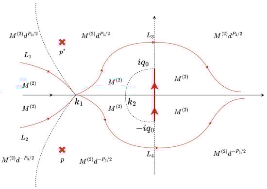
Figure 6. Diagram of the third deformation.

At this time, the jump conditions are

$$\begin{array}{cc}\hfill \forall k\in L_j, M^{\left(3\right)+}=& M^{\left(3\right)-}{V}_j^{\left(3\right)}, j=1,\dots ,4,\hfill \\ \hfill \forall k\in B, M^{\left(3\right)+}=& M^{\left(3\right)-}{V}_B^{\left(3\right)},\hfill \end{array}$$

(73)

where

$$\begin{array}{c}\hfill V_B^{\left(3\right)}=\left(\begin{array}{cc}0& {\displaystyle \frac{q_{-}}{i{q}_0}}{\delta }^2\\ {\displaystyle \frac{q_{-}^{*}}{i{q}_0}}{\delta }^{-2}& 0\end{array}\right), V_1^{\left(3\right)}=\left(\begin{array}{cc}1& {\displaystyle \frac{\overline{r}{e}^{2i\theta t}}{1+r\overline{r}}}{\delta }^2\\ 0& 1\end{array}\right), V_2^{\left(3\right)}=\left(\begin{array}{cc}1& 0\\ {\displaystyle \frac{r{e}^{-2i\theta t}}{1+r\overline{r}}}{\delta }^{-2}& 1\end{array}\right),\\ \hfill V_3^{\left(3\right)}=\left(\begin{array}{cc}1& 0\\ r{e}^{-2i\theta t}{\delta }^{-2}& 1\end{array}\right), V_4^{\left(3\right)}=\left(\begin{array}{cc}1& \overline{r}{e}^{2i\theta t}{\delta }^2\\ 0& 1\end{array}\right).\end{array}$$

(74)

Denote

$$\begin{array}{c}\hfill A_p^{\left(3\right)}=A_p^{\left(2\right)}{\left(d\left(p\right)\right)}^{-1}, B_p^{\left(3\right)}=B_p^{\left(2\right)}-{\left[2d\left(p\right)\right]}^{-1},\\ \hfill {\widehat{A}}_p^{\left(3\right)}={\widehat{A}}_p^{\left(2\right)}{\left(d\left(p^{*}\right)\right)}^{-1}, {\widehat{B}}_p^{\left(3\right)}={\widehat{B}}_p^{\left(2\right)}-{\left[2d\left(p^{*}\right)\right]}^{-1}.\end{array}$$

(75)

Then, the coefficient matrices in the series conditions are

$$\begin{array}{c}\hfill N_1^{\left(3\right)}=\left(\begin{array}{cc}0& A_p^{\left(3\right)}{e}^{2i\theta (\xi ,p)t}\\ 0& 0\end{array}\right), N_2^{\left(3\right)}=\left(\begin{array}{cc}0& A_p^{\left(3\right)}{e}^{2i\theta (\xi ,p)t}[B_p^{\left(3\right)}+2i{\theta }^{\prime }(\xi ,p)t]\\ 0& 0\end{array}\right),\\ \hfill {\widehat{N}}_1^{\left(3\right)}=\left(\begin{array}{cc}0& 0\\ {\widehat{A}}_p^{\left(3\right)}{e}^{-2i\theta (\xi ,p^{*})t}& 0\end{array}\right), {\widehat{N}}_2^{\left(3\right)}=\left(\begin{array}{cc}0& 0\\ {\widehat{A}}_p^{\left(3\right)}{e}^{-2i\theta (\xi ,p^{*})t}[{\widehat{B}}_p^{\left(3\right)}-2i{\theta }^{\prime }(\xi ,p^{*})t]& 0\end{array}\right).\end{array}$$

(76)

The asymptotic condition is

$$\underset{k\to \infty }{lim}{M}^{\left(3\right)}(x,t,k)=I+O\left({\displaystyle \frac{1}{k}}\right).$$

(77)

Fourth Deformation.${\mathrm{ V}}_B^{\left(3\right)}$ can be turned to a constant matrix by a transform

$$M^{\left(4\right)}(x,t,k)=M^{\left(3\right)}(x,t,k)e^{ig(\xi ,k)P_3},$$

(78)

where $g(\xi ,k)$ is analytic in $\mathbb{C}\setminus B$ and satisfies the Riemann–Hilbert problem

$$\begin{array}{cc}\hfill e^{i(g^{+}+g^{-})}& ={\delta }^2, \forall k\in B,\hfill \\ \hfill {\displaystyle \frac{g}{\lambda }}& =O(1/k), k\to \infty .\hfill \end{array}$$

(79)

The exact solution of (79) obtained by the Plemelj formula is

$$g(\xi ,k)={\displaystyle \frac{\lambda \left(k\right)}{2i{\pi }^2}}\sum _{\xi \in B}{\displaystyle \frac{1}{\lambda \left(\xi \right)(\xi -k)}}{\int }_{-\infty }^{k_1\left(\xi \right)}{\displaystyle \frac{ln(1+r\left(v\right)\overline{r}\left(v\right))}{v-\xi }}dv.$$

(80)

At this time, the jump conditions are

$$\begin{array}{cc}\hfill \forall k\in L_j, M^{\left(4\right)+}=& M^{\left(4\right)-}{V}_j^{\left(4\right)}, j=1,\dots ,4,\hfill \\ \hfill \forall k\in B, M^{\left(4\right)+}=& M^{\left(4\right)-}{V}_B^{\left(4\right)},\hfill \end{array}$$

(81)

where

$$\begin{array}{c}\hfill V_B^{\left(4\right)}=\left(\begin{array}{cc}0& {\displaystyle \frac{q_{-}}{i{q}_0}}\\ {\displaystyle \frac{q_{-}^{*}}{i{q}_0}}& 0\end{array}\right), V_1^{\left(4\right)}=\left(\begin{array}{cc}1& {\displaystyle \frac{\overline{r}{e}^{2i(\theta t-g)}}{1+r\overline{r}}}{\delta }^2\\ 0& 1\end{array}\right), V_2^{\left(4\right)}=\left(\begin{array}{cc}1& 0\\ {\displaystyle \frac{r{e}^{-2i(\theta t-g)}}{1+r\overline{r}}}{\delta }^{-2}& 1\end{array}\right),\\ \hfill V_3^{\left(4\right)}=\left(\begin{array}{cc}1& 0\\ r{e}^{-2i(\theta t-g)}{\delta }^{-2}& 1\end{array}\right), V_4^{\left(4\right)}=\left(\begin{array}{cc}1& \overline{r}{e}^{2i(\theta t-g)}{\delta }^2\\ 0& 1\end{array}\right).\end{array}$$

(82)

Denote

$$\begin{array}{c}\hfill A_p^{\left(4\right)}=A_p^{\left(3\right)}{e}^{-2ig(\xi ,p)}, B_p^{\left(4\right)}=B_p^{\left(3\right)}-i{g}^{\prime }(\xi ,p),\\ \hfill {\widehat{A}}_p^{\left(4\right)}={\widehat{A}}_p^{\left(3\right)}{e}^{2ig(\xi ,p^{*})}, {\widehat{B}}_p^{\left(4\right)}={\widehat{B}}_p^{\left(3\right)}+i{g}^{\prime }(\xi ,p^{*}).\end{array}$$

(83)

Then, the coefficient matrices in the series conditions are

$$\begin{array}{c}\hfill N_1^{\left(4\right)}=\left(\begin{array}{cc}0& A_p^{\left(4\right)}{e}^{2i\theta (\xi ,p)t}\\ 0& 0\end{array}\right), N_2^{\left(4\right)}=\left(\begin{array}{cc}0& A_p^{\left(4\right)}{e}^{2i\theta (\xi ,p)t}[B_p^{\left(4\right)}+2i{\theta }^{\prime }(\xi ,p)t]\\ 0& 0\end{array}\right),\\ \hfill {\widehat{N}}_1^{\left(4\right)}=\left(\begin{array}{cc}0& 0\\ {\widehat{A}}_p^{\left(4\right)}{e}^{-2i\theta (\xi ,p^{*})t}& 0\end{array}\right), {\widehat{N}}_2^{\left(4\right)}=\left(\begin{array}{cc}0& 0\\ {\widehat{A}}_p^{\left(4\right)}{e}^{-2i\theta (\xi ,p^{*})t}[{\widehat{B}}_p^{\left(4\right)}-2i{\theta }^{\prime }(\xi ,p^{*})t]& 0\end{array}\right).\end{array}$$

(84)

Define

$$g_{\infty }\left(\xi \right)=\underset{k\to \infty }{lim}g(\xi ,k)={\displaystyle \frac{1}{2i{\pi }^2}}\sum _{\xi \in B}{\displaystyle \frac{1}{\lambda \left(\xi \right)}}{\int }_{-\infty }^{k_1\left(\xi \right)}{\displaystyle \frac{ln\left[1+r\left(v\right)\overline{r}\left(v\right)\right]}{v-\xi }}dv.$$

(85)

Because ${\left(\lambda \left(k\right)\right)}^{*}=\lambda \left(k^{*}\right),{\left(\delta (\xi ,k)\right)}^{*}={\left[\delta (\xi ,k^{*})\right]}^{-1}$, the symmetry holds ${\left(g_{\infty }\left(\xi \right)\right)}^{*}=g_{\infty }\left(\xi \right)$, namely, $g_{\infty }\in \mathbb{R}$.

At this time, the asymptotic condition is

$$\underset{k\to \infty }{lim}{M}^{\left(4\right)}(x,t,k)=e^{i{g}_{\infty }\left(\xi \right)P_3}+O\left({\displaystyle \frac{1}{k}}\right).$$

(86)

Substituting the progress of the deformation into (36), we have

$$q(x,t)=\underset{k\to \infty }{lim}-ik{M}_{1,2}^{\left(4\right)}(x,t,k)e^{i{g}_{\infty }\left(\xi \right)}.$$

(87)

Now the jump matrices of (74) except for $V_B$ tend to zero as $t\to \infty$ and the coefficient matrices in (84) tend to zero as $t\to \infty$. So when $\xi <v_s$, the dominant component of $M^{\left(4\right)}(x,t,k)$, denoted as $M^{\mathrm{dom}}(x,t,k)$, satisfies the following Riemann–Hilbert problem

$$\begin{array}{cc}\hfill M^{\mathrm{dom}+}& =M^{\mathrm{dom}-}{V}_B^{\left(4\right)}, \forall k\in B,\hfill \\ \hfill M^{\mathrm{dom}}& =e^{i{g}_{\infty }\left(\xi \right)P_3}+O\left({\displaystyle \frac{1}{k}}\right).\hfill \end{array}$$

(88)

The solution can be obtained by the Plemelj formula after diagonalizing the matrix function $M^{\mathrm{dom}}$

$$M^{\mathrm{dom}}={\displaystyle \frac{1}{2}}{e}^{i{g}_{\infty }\left(\xi \right)P_3}\left(\begin{array}{cc}\mathsf{\Lambda }\left(k\right)+{\mathsf{\Lambda }}^{-1}\left(k\right)& -{\displaystyle \frac{q_0}{q_{-}^{*}}}\left[\mathsf{\Lambda }\left(k\right)-{\mathsf{\Lambda }}^{-1}\left(k\right)\right]\\ -{\displaystyle \frac{q_0}{q_{-}}}\left[\mathsf{\Lambda }\left(k\right)-{\mathsf{\Lambda }}^{-1}\left(k\right)\right]& \mathsf{\Lambda }\left(k\right)+{\mathsf{\Lambda }}^{-1}\left(k\right)\end{array}\right), \mathrm{where} \mathsf{\Lambda }\left(k\right)={\left({\displaystyle \frac{k-i{q}_0}{k+i{q}_0}}\right)}^{{\displaystyle \frac{1}{4}}}.$$

(89)

Substituting (89) into (87), the dominant component of $q(x,t)$ can be obtained as

$$q(x,t)\sim q^{\mathrm{dom}}=\underset{k\to \infty }{lim}-ik{M}_{1,2}^{\mathrm{dom}}(x,t,k)e^{i{g}_{\infty }\left(\xi \right)}=q_{-}{e}^{2i{g}_{\infty }\left(\xi \right)}.$$

(90)

Because $g_{\infty }\left(\xi \right)$ is a real number for $\xi <v_0$, we have $\left|q(x,t)\right|\sim q_{-}$. This resembles the asymptotic result when there is only a continuous spectrum without a discrete spectrum [16]. In this case, only the time terms in the elimination of the jump conditions are considered in the deformation, while the coefficients of the series conditions automatically vanish when $t\to \infty$. The addition of the series conditions has no impact on the result. However, the situation is different for $\xi >v_s$, because then the adjustment of the time terms in the series conditions must be considered.

4.2. $\xi \in (v_s,v_0)$

Fifth Deformation. When $\xi \in (v_s,v_0)$, p is to the right of $\mathrm{Re}\left[i\theta (v_0,k)\right]=0$. As $t\to \infty$, the time terms in the series conditions tend to infinity. They can be adjusted by the transformation

$$M^{\left(5\right)}(x,t,k)=M^{\left(4\right)}(x,t,k)n{\left(k\right)}^{P_3},$$

(91)

where $n\left(k\right)={\left({\displaystyle \frac{k-p^{*}}{k-p}}\right)}^2$. The jump conditions become

$$\begin{array}{cc}\hfill \forall k\in L_j, M^{\left(5\right)+}=& M^{\left(5\right)-}{V}_j^{\left(5\right)}, j=1,\dots ,4,\hfill \\ \hfill \forall k\in B, M^{\left(5\right)+}=& M^{\left(5\right)-}{V}_B^{\left(5\right)},\hfill \end{array}$$

(92)

where

$$\begin{array}{c}\hfill V_B^{\left(5\right)}=\left(\begin{array}{cc}0& {\displaystyle \frac{q_{-}}{i{q}_0}}{n}^{-2}\\ {\displaystyle \frac{q_{-}^{*}}{i{q}_0}}{n}^2& 0\end{array}\right), V_1^{\left(5\right)}=\left(\begin{array}{cc}1& {\displaystyle \frac{\overline{r}{e}^{2i(\theta t-g)}}{1+r\overline{r}}}{\delta }^2{n}^{-2}\\ 0& 1\end{array}\right), V_2^{\left(5\right)}=\left(\begin{array}{cc}1& 0\\ {\displaystyle \frac{r{e}^{-2i(\theta t-g)}}{1+r\overline{r}}}{\delta }^{-2}{n}^2& 1\end{array}\right),\\ \hfill V_3^{\left(5\right)}=\left(\begin{array}{cc}1& 0\\ r{e}^{-2i(\theta t-g)}{\delta }^{-2}{n}^2& 1\end{array}\right), V_4^{\left(5\right)}=\left(\begin{array}{cc}1& \overline{r}{e}^{2i(\theta t-g)}{\delta }^2{n}^{-2}\\ 0& 1\end{array}\right).\end{array}$$

(93)

The asymptotic condition is

$$\underset{k\to \infty }{lim}{M}^{\left(5\right)}(x,t,k)=e^{i{g}_{\infty }\left(\xi \right)P_3}+O\left({\displaystyle \frac{1}{k}}\right).$$

(94)

We still need to analyze the series conditions.

The Laurent expansion of $n\left(k\right)$ at $k=p$ is

$$n\left(k\right)={\displaystyle \frac{a_{-2}}{{(k-p)}^2}}+{\displaystyle \frac{a_{-1}}{k-p}}+O\left(1\right),$$

(95)

where

$$a_{-2}={(p-p^{*})}^2,a_{-1}=-2(p-p^{*}).$$

(96)

Thus, the Laurent expansion of ${\displaystyle \frac{1}{n\left(k\right)}}$ at $k=p$ is

$${\displaystyle \frac{1}{n\left(k\right)}}={(k-p)}^2\left[{\displaystyle \frac{1}{a_{-2}}}-{\displaystyle \frac{a_{-1}}{a_{-2}^2}}(k-p)+O\left({(k-p)}^2\right)\right].$$

(97)

We use subscript j to represent the columns of the matrix, i.e., $M^{\left(4\right)}(x,t,k)=\left[M_1^{\left(4\right)}(x,t,k),M_2^{\left(4\right)}(x,t,k)\right]$. According to the series conditions (84), expansion of $M_2^{\left(4\right)}(x,t,k)$ goes down to the second-order. We perform a Laurent expansion of $M_2^{\left(5\right)}(x,t,k)$ around $k=p$ and substitute it into the series conditions. For the sake of notation simplicity, x and t are omitted in the following expressions.

$$\begin{array}{cc}\hfill M_2^{\left(5\right)}\left(k\right)=& M_2^{\left(4\right)}{n}^{-1}\left(k\right)\hfill \\ \hfill =& \left[{\displaystyle \frac{P_{-2}{M}_2^{\left(4\right)}}{{(k-p)}^2}}+{\displaystyle \frac{Res{M}_2^{\left(4\right)}}{(k-p)}}+O\left(1\right)\right]{(k-p)}^2\left[{\displaystyle \frac{1}{a_{-2}}}-{\displaystyle \frac{a_{-1}}{a_{-2}^2}}(k-p)+O\left({(k-p)}^2\right)\right]\hfill \\ \hfill =& {\displaystyle \frac{A_p^{\left(4\right)}{e}^{2i\theta t}}{a_{-2}}}{M}_1^{\left(4\right)}\left(p\right)\hfill \\ \hfill & +{\left(a_{-2}\right)}^{-1}{A}_p^{\left(4\right)}{e}^{2i\theta t}\left[{\left(M_1^{\left(4\right)}\right)}^{\prime }\left(p\right)+(B_p^{\left(4\right)}-{\displaystyle \frac{a_{-1}}{a_{-2}}}+2i{\theta }^{\prime }(\xi ,p)t)M_1^{\left(4\right)}\left(p\right)\right](k-p)\hfill \\ \hfill & +O\left[{(k-p)}^2\right].\hfill \end{array}$$

(98)

Therefore, we have the following series conditions

$$\underset{k=p}{P_{-2}}{M}_2^{\left(5\right)}=0, \underset{k=p}{Res}{M}_2^{\left(5\right)}=0,$$

(99)

and

$$\begin{array}{cc}\hfill M_2^{\left(5\right)}\left(p\right)& ={\displaystyle \frac{A_p^{\left(4\right)}{e}^{2i\theta t}}{a_{-2}}}{M}_1^{\left(4\right)}\left(p\right),\hfill \\ \hfill {\left(M_2^{\left(5\right)}\right)}^{\prime }\left(p\right)& ={\left(a_{-2}\right)}^{-1}{A}_p^{\left(4\right)}{e}^{2i\theta t}\left[{\left(M_1^{\left(4\right)}\right)}^{\prime }\left(p\right)+(B_p^{\left(4\right)}-{\displaystyle \frac{a_{-1}}{a_{-2}}}+2i{\theta }^{\prime }(\xi ,p)t)M_1^{\left(4\right)}\left(p\right)\right].\hfill \end{array}$$

(100)

Similarly, we perform the Laurent expansion of $M_1^{\left(5\right)}(x,t,k)$ around $k=p$,

$$\begin{array}{cc}\hfill M_1^{\left(5\right)}\left(k\right)=& M_1^{\left(4\right)}\left(k\right)n\left(k\right)\hfill \\ \hfill =& \left[M_1^{\left(4\right)}\left(p\right)+{\left(M_1^{\left(4\right)}\right)}^{\prime }\left(p\right)(k-p)+O\left({(k-p)}^2\right)\right]\left[{\displaystyle \frac{a_{-2}}{{(k-p)}^2}}+{\displaystyle \frac{a_{-1}}{k-p}}+O\left(1\right)\right]\hfill \\ \hfill =& a_{-2}{M}_1^{\left(4\right)}{(k-p)}^{-2}+\left[a_{-1}{M}_1^{\left(4\right)}\left(p\right)+a_{-2}{\left(M_1^{\left(4\right)}\right)}^{\prime }\left(p\right)\right]{(k-p)}^{-1}+O\left(1\right).\hfill \end{array}$$

(101)

Therefore, we have the series conditions

$$\begin{array}{cc}\hfill \underset{k=p}{P_{-2}}{M}_1^{\left(5\right)}& =a_{-2}{M}_1^{\left(4\right)}\left(p\right),\hfill \\ \hfill \underset{k=p}{Res}{M}_1^{\left(5\right)}& =a_{-1}{M}_1^{\left(4\right)}\left(p\right)+a_{-2}{\left(M_1^{\left(4\right)}\right)}^{\prime }\left(p\right).\hfill \end{array}$$

(102)

Substituting (100) and (96) into (102), we get the series conditions

$$\begin{array}{cc}\hfill \underset{k=p}{P_{-2}}{M}_1^{\left(5\right)}=& {(p-p^{*})}^2{\left(A_p^{\left(4\right)}\right)}^{-1}{M}_1^{\left(5\right)},\hfill \\ \hfill \underset{k=p}{Res}{M}_1^{\left(5\right)}=& {(p-p^{*})}^4{\left(A_p^{\left(4\right)}\right)}^{-1}{e}^{-2i\theta t}{\left(M_2^{\left(5\right)}\right)}^{\prime }\left(p\right)\hfill \\ \hfill & +{(p-p^{*})}^4{\left(A_p^{\left(4\right)}\right)}^{-1}{e}^{-2i\theta t}\left[{\displaystyle \frac{4}{p-p^{*}}}-B_p^{\left(4\right)}-2i{\theta }^{\prime }(\xi ,p)t\right]M_2^{\left(5\right)}.\hfill \end{array}$$

(103)

Similarly, we may show that

$$\begin{array}{cc}\hfill \underset{k=p^{*}}{P_{-2}}{M}_1^{\left(5\right)}=& 0,\hfill \\ \hfill \underset{k=p^{*}}{Res}{M}_1^{\left(5\right)}=& 0,\hfill \\ \hfill \underset{k=p^{*}}{P_{-2}}{M}_2^{\left(5\right)}=& {(p-p^{*})}^2{\left({\widehat{A}}_p^{\left(4\right)}\right)}^{-1}{M}_2^{\left(5\right)},\hfill \\ \hfill \underset{k=p^{*}}{Res}{M}_2^{\left(5\right)}=& {(p-p^{*})}^4{\left({\widehat{A}}_p^{\left(4\right)}\right)}^{-1}{e}^{2i\theta t}{\left(M_1^{\left(5\right)}\right)}^{\prime }\left(p\right)\hfill \\ \hfill & +{(p-p^{*})}^4{\left({\widehat{A}}_p^{\left(4\right)}\right)}^{-1}{e}^{2i\theta t}\left[{\displaystyle \frac{4}{p-p^{*}}}-{\widehat{B}}_p^{\left(4\right)}+2i{\theta }^{\prime }(\xi ,p^{*})t\right]M_1^{\left(5\right)}.\hfill \end{array}$$

(104)

Combining (99), (103) and (104), we get the series condition

$$\begin{array}{c}\hfill A_p^{\left(5\right)}={\left(A_p^{\left(4\right)}\right)}^{-1}{(p-p^{*})}^4, B_p^{\left(5\right)}={\displaystyle \frac{4}{p^{*}-p}}-B_p^{\left(4\right)},\\ \hfill {\widehat{A}}_p^{\left(5\right)}={\left({\widehat{A}}_p^{\left(4\right)}\right)}^{-1}{(p-p^{*})}^4, {\widehat{B}}_p^{\left(5\right)}={\displaystyle \frac{4}{p-p^{*}}}-{\widehat{B}}_p^{\left(4\right)}.\end{array}$$

(105)

Then the corresponding coefficient matrices are

$$\begin{array}{c}\hfill N_1^{\left(5\right)}=\left(\begin{array}{cc}0& 0\\ A_p^{\left(5\right)}{e}^{-2i\theta (\xi ,p)t}& 0\end{array}\right), N_2^{\left(5\right)}=\left(\begin{array}{cc}0& 0\\ A_p^{\left(5\right)}{e}^{-2i\theta (\xi ,p)t}[B_p^{\left(5\right)}-2i{\theta }^{\prime }(\xi ,p)t]& 0\end{array}\right),\\ \hfill {\widehat{N}}_1^{\left(5\right)}=\left(\begin{array}{cc}0& {\widehat{A}}_p^{\left(5\right)}{e}^{2i\theta (\xi ,p^{*})t}\\ 0& 0\end{array}\right), {\widehat{N}}_2^{\left(5\right)}=\left(\begin{array}{cc}0& {\widehat{A}}_p^{\left(5\right)}{e}^{2i\theta (\xi ,p^{*})t}[{\widehat{B}}_p^{\left(5\right)}+2i{\theta }^{\prime }(\xi ,p^{*})t]\\ 0& 0\end{array}\right).\end{array}$$

(106)

Sixth Deformation. Similar to the fourth deformation, $V_B^{\left(5\right)}$ can be turned to a constant matrix by the transformation

$$M^{\left(6\right)}(x,t,k)=M^{\left(5\right)}(x,t,k)e^{i\tilde{g}(\xi ,k)P_3},$$

(107)

where $\tilde{g}(\xi ,k)$ is analytic in $\mathbb{C}\setminus B$, and satisfies the Riemann–Hilbert problem

$$\begin{array}{cc}\hfill e^{i({\tilde{g}}^{+}+{\tilde{g}}^{-})}& =n^{-2}, \forall k\in B,\hfill \\ \hfill {\displaystyle \frac{\tilde{g}}{\lambda }}& =O(1/k), k\to \infty .\hfill \end{array}$$

(108)

The exact solution of (108) can be obtained by the Plemelj formula

$$\tilde{g}\left(k\right)=-{\displaystyle \frac{\lambda \left(k\right)}{\pi }}{\int }_{\xi \in B}{\displaystyle \frac{ln\left(n\right(\xi \left)\right)}{\lambda \left(\xi \right)(\xi -k)}}d\xi .$$

(109)

At this time, the jump conditions are

$$\begin{array}{cc}\hfill \forall k\in L_j, M^{\left(6\right)+}=& M^{\left(6\right)-}{V}_j^{\left(6\right)}, j=1,\dots ,4,\hfill \\ \hfill \forall k\in B, M^{\left(6\right)+}=& M^{\left(6\right)-}{V}_B^{\left(6\right)},\hfill \end{array}$$

(110)

where

$$\begin{array}{c}\hfill V_B^{\left(6\right)}=\left(\begin{array}{cc}0& {\displaystyle \frac{q_{-}}{i{q}_0}}\\ {\displaystyle \frac{q_{-}^{*}}{i{q}_0}}& 0\end{array}\right), V_1^{\left(6\right)}=\left(\begin{array}{cc}1& {\displaystyle \frac{\overline{r}{e}^{2i(\theta t-g-\tilde{g})}}{1+r\overline{r}}}{\delta }^2{n}^{-2}\\ 0& 1\end{array}\right), V_2^{\left(6\right)}=\left(\begin{array}{cc}1& 0\\ {\displaystyle \frac{r{e}^{-2i(\theta t-g-\tilde{g})}}{1+r\overline{r}}}{\delta }^{-2}{n}^2& 1\end{array}\right),\\ \hfill V_3^{\left(6\right)}=\left(\begin{array}{cc}1& 0\\ r{e}^{-2i(\theta t-g-\tilde{g})}{\delta }^{-2}{n}^2& 1\end{array}\right), V_4^{\left(6\right)}=\left(\begin{array}{cc}1& \overline{r}{e}^{2i(\theta t-g-\tilde{g})}{\delta }^2{n}^{-2}\\ 0& 1\end{array}\right).\end{array}$$

(111)

Let

$$\begin{array}{c}\hfill A_p^{\left(6\right)}=A_p^{\left(5\right)}{e}^{2i\tilde{g}\left(p\right)}, B_p^{\left(6\right)}=B_p^{\left(5\right)}+i{\tilde{g}}^{\prime }\left(p\right),\\ \hfill {\widehat{A}}_p^{\left(6\right)}={\widehat{A}}_p^{\left(5\right)}{e}^{-2i\tilde{g}\left(p^{*}\right)}, {\widehat{B}}_p^{\left(6\right)}={\widehat{B}}_p^{\left(5\right)}-i{\tilde{g}}^{\prime }\left(p^{*}\right),\end{array}$$

(112)

the coefficient matrices in the series conditions are

$$\begin{array}{c}\hfill N_1^{\left(6\right)}=\left(\begin{array}{cc}0& 0\\ A_p^{\left(6\right)}{e}^{-2i\theta (\xi ,p)t}& 0\end{array}\right), N_2^{\left(6\right)}=\left(\begin{array}{cc}0& 0\\ A_p^{\left(6\right)}{e}^{-2i\theta (\xi ,p)t}[B_p^{\left(6\right)}-2i{\theta }^{\prime }(\xi ,p)t]& 0\end{array}\right),\\ \hfill {\widehat{N}}_1^{\left(6\right)}=\left(\begin{array}{cc}0& {\widehat{A}}_p^{\left(6\right)}{e}^{2i\theta (\xi ,p^{*})t}\\ 0& 0\end{array}\right), {\widehat{N}}_2^{\left(6\right)}=\left(\begin{array}{cc}0& {\widehat{A}}_p^{\left(6\right)}{e}^{2i\theta (\xi ,p^{*})t}[{\widehat{B}}_p^{\left(6\right)}+2i{\theta }^{\prime }(\xi ,p^{*})t]\\ 0& 0\end{array}\right).\end{array}$$

(113)

Define

$$\begin{array}{c}\hfill {\tilde{g}}_{\infty }=\underset{k\to \infty }{lim}\tilde{g}\left(k\right)=4\arg \left[p+\lambda \left(p\right)\right].\end{array}$$

(114)

The asymptotic condition is

$$\underset{k\to \infty }{lim}{M}^{\left(6\right)}(x,t,k)=e^{i(g_{\infty }\left(\xi \right)+{\tilde{g}}_{\infty })P_3}+O\left({\displaystyle \frac{1}{k}}\right).$$

(115)

The solution of the nonlinear Schrödinger equation is

$$\begin{array}{cc}\hfill q(x,t)& =\underset{k\to \infty }{lim}-ik{M}_{1,2}^{\left(6\right)}(x,t,k)e^{i{\tilde{g}}_{\infty }}\hfill \\ \hfill & =\underset{k\to \infty }{lim}-ik{M}_{1,2}^{\left(4\right)}(x,t,k)e^{i(g_{\infty }\left(\xi \right)+{\tilde{g}}_{\infty })}.\hfill \end{array}$$

(116)

Comparing (116) and (87), we observe that for $\xi \in (v_s,v_0)$, p is to the right of $\mathrm{Re}\left[i\theta (v_0,k)\right]=0$, and the asymptotic behavior of the time terms in the series condition changes. This results in a fixed phase offset $e^{2i{\tilde{g}}_{\infty }}$ for the solution of the nonlinear Schrödinger equation. At this time, the dominant component of $q(x,t)$ is

$$q(x,t)\sim q_{-}{e}^{2i\left[g_{\infty }\left(\xi \right)+{\tilde{g}}_{\infty }\right]}.$$

(117)

4.3. $\xi \in (v_0,0)$

The curve $\mathrm{Re}\left[i\theta (v_0,k)\right]=0$ does not intersect the real axis. Following Biondini’s approach to study the asymptotic behavior with continuous spectra [18], we assume that $k_0\left(\xi \right)$ represents an undetermined point on the negative real axis, with $\xi$ as the independent variable. We shall replace the position of $k_1\left(\xi \right)$ in the first deformation with $k_0\left(\xi \right)$ for the subsequent transformations.

Seventh Deformation. Similar to the first deformation, the values of different regions after the seventh deformation are shown in Figure 7.

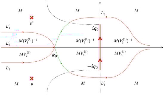
Figure 7. Diagram of the seventh deformation.

The jump conditions are

$$\begin{array}{cc}\hfill \forall k\in L_j, M^{\left(7\right)+}=& M^{\left(7\right)-}{V}_j^{\left(7\right)}, j=0,\dots ,4,\hfill \\ \hfill \forall k\in B, M^{\left(7\right)+}=& M^{\left(7\right)-}{V}_B^{\left(7\right)},\hfill \end{array}$$

(118)

where the jump matrices are the same as (62). The value of the function at p and $p^{*}$ remains unchanged, so the series coefficients are the same as (48) and (50), namely, $N_1^{\left(7\right)}=N_1^{\left(1\right)}, N_2^{\left(7\right)}=N_2^{\left(1\right)}, {\widehat{N}}_1^{\left(7\right)}={\widehat{N}}_1^{\left(1\right)}, {\widehat{N}}_2^{\left(7\right)}={\widehat{N}}_2^{\left(1\right)}$.

The asymptotic condition is

$$\underset{k\to \infty }{lim}{M}^{\left(7\right)}(x,t,k)=I+O\left({\displaystyle \frac{1}{k}}\right).$$

(119)

Eighth Deformation. Similar to the second deformation, the jump $V_0^{\left(7\right)}$ along $L_0$ can be removed by the transformation

$$M^{\left(8\right)}(x,t,k)=M^{\left(7\right)}(x,t,k){\delta }_0^{-P_3}, \mathrm{where} {\delta }_0(\xi ,k)=exp\left\{{\displaystyle \frac{1}{2\pi i}}{\int }_{\infty }^{k_0\left(\xi \right)}{\displaystyle \frac{ln[1+r\left(v\right)\overline{r}\left(v\right)]}{v-k}}dv\right\}.$$

(120)

The jump conditions become

$$\begin{array}{cc}\hfill \forall k\in L_j, M^{\left(8\right)+}=& M^{\left(8\right)-}{V}_j^{\left(8\right)}, j=1,\dots ,4,\hfill \\ \hfill \forall k\in B, M^{\left(8\right)+}=& M^{\left(8\right)-}{V}_B^{\left(8\right)},\hfill \end{array}$$

(121)

where the step matrices are similar to those in the second deformation (69), except $\delta (\xi ,k)$ is replaced by ${\delta }_0(\xi ,k)$. The coefficient matrices in the series conditions are similar to (71), except that $\delta (\xi ,k)$ in $A_p^{\left(2\right)},B_p^{\left(2\right)},{\widehat{A}}_p^{\left(2\right)},{\widehat{B}}_p^{\left(2\right)}$ is replaced by ${\delta }_0(\xi ,k)$, giving $A_p^{\left(8\right)},B_p^{\left(8\right)},{\widehat{A}}_p^{\left(8\right)},{\widehat{B}}_p^{\left(8\right)}$.

The asymptotic condition is

$$\underset{k\to \infty }{lim}{M}^{\left(8\right)}(x,t,k)=I+O\left({\displaystyle \frac{1}{k}}\right).$$

(122)

Ninth Deformation. Similar to the third deformation, the function $d\left(k\right)$ can be eliminated by defining $M^{\left(9\right)}(x,t,k)$ as shown in Figure 8.

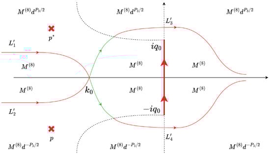
Figure 8. Diagram of the ninth deformation.

The jump conditions are

$$\begin{array}{cc}\hfill \forall k\in L_j, M^{\left(9\right)+}=& M^{\left(9\right)-}{V}_j^{\left(9\right)}, j=1,\dots ,4,\hfill \\ \hfill \forall k\in B, M^{\left(9\right)+}=& M^{\left(9\right)-}{V}_B^{\left(9\right)},\hfill \end{array}$$

(123)

where the step matrices are similar to those in the third deformation (74), except that $\delta (\xi ,k)$ is replaced by ${\delta }_0(\xi ,k)$. The coefficient matrices in the series conditions are similar to (76), except that $\delta (\xi ,k)$ in $A_p^{\left(3\right)},B_p^{\left(3\right)},{\widehat{A}}_p^{\left(3\right)},{\widehat{B}}_p^{\left(3\right)}$ is replaced by ${\delta }_0(\xi ,k)$, giving $A_p^{\left(9\right)},B_p^{\left(9\right)},{\widehat{A}}_p^{\left(9\right)},{\widehat{B}}_p^{\left(9\right)}$.

The asymptotic condition is

$$\underset{k\to \infty }{lim}{M}^{\left(9\right)}(x,t,k)=I+O\left({\displaystyle \frac{1}{k}}\right).$$

(124)

Tenth Deformation. In Figure 8, the dashed line represents the equation $\mathrm{Re}\left[i\theta (v_0,k)\right]=0$. Therefore, in the green segment of $L_3^{\prime }$ and $L_4^{\prime }$ from $k_0$ to the dashed line, the time terms in the step matrices tend to infinity as $t\to \infty$. Decompose the jump matrices to deal with the time terms as follows

$$V_3^{\left(9\right)}=V_5^{\left(10\right)}{V}_7^{\left(10\right)}{V}_5^{\left(10\right)}, V_4^{\left(9\right)}=V_6^{\left(10\right)}{V}_8^{\left(10\right)}{V}_6^{\left(10\right)},$$

(125)

where

$$\begin{array}{c}\hfill V_5^{\left(10\right)}=\left(\begin{array}{cc}1& {\displaystyle \frac{{\delta }_0^2}{r}}{e}^{2i\theta t}\\ 0& 1\end{array}\right), V_6^{\left(10\right)}=\left(\begin{array}{cc}1& 0\\ {\displaystyle \frac{1}{\overline{r}{\delta }_0^2}}{e}^{-2i\theta t}& 1\end{array}\right),\\ \hfill V_7^{\left(10\right)}=\left(\begin{array}{cc}0& -{\displaystyle \frac{{\delta }_0^2}{r}}{e}^{2i\theta t}\\ {\displaystyle \frac{r}{{\delta }_0^2}}{e}^{-2i\theta t}& 0\end{array}\right), V_8^{\left(10\right)}=\left(\begin{array}{cc}1& \overline{r}{\delta }_0^2{e}^{2i\theta t}\\ -{\displaystyle \frac{1}{\overline{r}{\delta }_0^2}}{e}^{-2i\theta t}& 1\end{array}\right).\end{array}$$

(126)

The values of $M^{\left(10\right)}(x,t,k)$ are defined as shown in Figure 9.

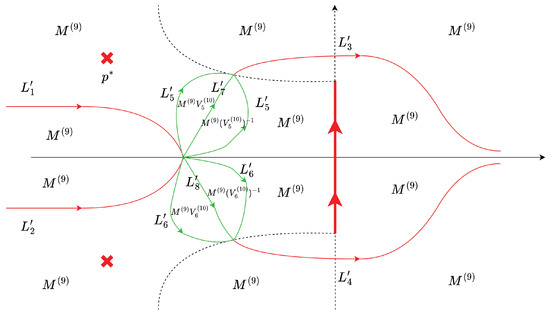
Figure 9. Diagram of the tenth deformation.

The jump conditions are

$$\begin{array}{cc}\hfill \forall k\in L_j, M^{\left(10\right)+}=& M^{\left(10\right)-}{V}_j^{\left(10\right)}, j=1,\dots ,8,\hfill \\ \hfill \forall k\in B, M^{\left(10\right)+}=& M^{\left(10\right)-}{V}_B^{\left(10\right)},\hfill \end{array}$$

(127)

where $V_j^{\left(10\right)}=V_j^{\left(9\right)},j=1,\dots ,4$, and other jump matrices are defined as (126). The coefficient matrices in the series conditions are the same as those in the ninth deformation.

Denote the intersection point of $L_7^{\prime }$ and $\mathrm{Re}\left[i\theta (v_0,k)\right]=0$ as $\alpha \left(\xi \right)$, and the intersection point of $L_8^{\prime }$ and $\mathrm{Re}\left[i\theta (v_0,k)\right]=0$ above in ${\alpha }^{*}\left(\xi \right)$. Let $\tilde{B}=L_7^{\prime }\cup (-L_8^{\prime })$. Then the curve $\tilde{B}$ starts from ${\alpha }^{*}\left(\xi \right)$, passes $k_0\left(\xi \right)$ and reaches $\alpha \left(\xi \right)$.

Eleventh Deformation. To eliminate the time terms growing to infinity in $V_7^{\left(10\right)}$ and $V_8^{\left(10\right)}$, we assume that there exists a discontinuous function $h(\xi ,k)$ on B and $\tilde{B}$. The transformation is

$$M^{\left(11\right)}(x,t,k)=M^{\left(10\right)}(x,t,k)e^{i\left[h\right(\xi ,t)-\theta (\xi ,t\left)\right]}.$$

(128)

The jump conditions are

$$\begin{array}{cc}\hfill \forall k\in L_j, M^{\left(11\right)+}=& M^{\left(11\right)-}{V}_j^{\left(11\right)}, j=1,\dots ,8,\hfill \\ \hfill \forall k\in B, M^{\left(11\right)+}=& M^{\left(10\right)-}{V}_B^{\left(11\right)},\hfill \end{array}$$

(129)

where

$$\begin{array}{c}\hfill V_B^{\left(11\right)}=\left(\begin{array}{cc}0& {\displaystyle \frac{q_{-}}{i{q}_0}}{\delta }_0^2{e}^{i(h^{+}+h^{-})}\\ {\displaystyle \frac{q_{-}^{*}}{i{q}_0}}{e}^{-i(h^{+}+h^{-})}{\delta }_0^{-2}& 0\end{array}\right), V_1^{\left(11\right)}=\left(\begin{array}{cc}1& {\displaystyle \frac{\overline{r}{e}^{2iht}}{1+r\overline{r}}}{\delta }_0^2\\ 0& 1\end{array}\right), V_2^{\left(11\right)}=\left(\begin{array}{cc}1& 0\\ {\displaystyle \frac{r{e}^{-2iht}}{1+r\overline{r}}}{\delta }_0^{-2}& 1\end{array}\right),\\ \hfill V_3^{\left(11\right)}=\left(\begin{array}{cc}1& 0\\ r{e}^{-2iht}{\delta }_0^{-2}& 1\end{array}\right), V_4^{\left(11\right)}=\left(\begin{array}{cc}1& \overline{r}{e}^{2iht}{\delta }_0^2\\ 0& 1\end{array}\right), V_5^{\left(11\right)}=\left(\begin{array}{cc}1& {\displaystyle \frac{{\delta }_0^2}{r}}{e}^{2iht}\\ 0& 1\end{array}\right), V_6^{\left(11\right)}=\left(\begin{array}{cc}1& 0\\ {\displaystyle \frac{1}{\overline{r}{\delta }_0^2}}{e}^{-2iht}& 1\end{array}\right),\\ \hfill V_7^{\left(11\right)}=\left(\begin{array}{cc}0& -{\displaystyle \frac{{\delta }_0^2}{r}}{e}^{2i(h^{+}+h^{-})t}\\ {\displaystyle \frac{r}{{\delta }_0^2}}{e}^{-2i(h^{+}+h^{-})t}& 0\end{array}\right), V_8^{\left(11\right)}=\left(\begin{array}{cc}1& \overline{r}{\delta }_0^2{e}^{2i(h^{+}+h^{-})t}\\ -{\displaystyle \frac{1}{\overline{r}{\delta }_0^2}}{e}^{-2i(h^{+}+h^{-})t}& 1\end{array}\right).\end{array}$$

(130)

Here $h(\xi ,k)$ must satisfy the following conditions.

1.

$h^{+}+h^{-}=0, \forall k\in B$.

2.

$\mathrm{Re}(h^{+}+h^{-})=0, \forall k\in \tilde{B}$.

3.

$\mathrm{Re}\left[h(\xi ,k)\right]=\mathrm{Re}\left[\theta (\xi ,k)\right]+O\left({\displaystyle \frac{1}{k}}\right)$. This guarantees that $V_j^{\left(10\right)},(j=1,\dots ,6)$ uniformly tends to identity at the infinity point of k-plane.

4.

The sign of $\mathrm{Re}\left[h\right(\xi ,k\left)\right]$ is the same as that of $\mathrm{Re}\left[\theta \right(\xi ,k\left)\right]$ around the origin, $k=\alpha$ and $k={\alpha }^{*}$.

In the proof of the asymptotic behavior with the continuous spectrum [18], Biondini pointed out that the existence of such $h(\xi ,k)$ requires certain conditions on $k_0$ and $\alpha$. More precisely, denote ${\alpha }_{\mathrm{Re}}\left(\xi \right)=\mathrm{Re}\left[\alpha \left(\xi \right)\right]$ and ${\alpha }_{im}\left(\xi \right)=Im\left[\alpha \left(\xi \right)\right]$, and their values are uniquely determined by the following system of equations

$$\begin{array}{cc}\hfill {\displaystyle \frac{\xi }{2}}& =2{\alpha }_{\mathrm{Re}}+{\displaystyle \frac{q_0^2-{\alpha }_{im}^2}{{\alpha }_{\mathrm{Re}}}},\hfill \\ \hfill m^2& ={\displaystyle \frac{4q_0{\alpha }_{im}}{{\alpha }_{\mathrm{Re}}^2+{(q_0+{\alpha }_{im})}^2}},\hfill \\ \hfill [{\alpha }_{\mathrm{Re}}^2+{(q_0-{\alpha }_{im})}^2]K\left(m\right)& =({\alpha }_{\mathrm{Re}}^2-{\alpha }_{im}^2+q_0^2)E\left(m\right).\hfill \end{array}$$

(131)

Here m is an auxiliary variable. These conditions actually determine the appropriate values of $k_0$ and $\alpha$. We note that ${\alpha }^{*}\left(\xi \right)$ determines the boundary between $D_2^{+}$ and $D_2^{-}$ in Figure 1, the parametric curve $\left\{{\alpha }^{*}\left(\xi \right)|\xi \in (v_0,0)\right\}$. We have

$$\begin{array}{cc}\hfill k_0\left(\xi \right)& =-{\alpha }_{\mathrm{Re}}\left(\xi \right)+{\displaystyle \frac{\xi }{4}},\hfill \\ \hfill h(\xi ,k)& =-2\left({\int }_{i{q}_0}^k+{\int }_{-i{q}_0}^k\right){\displaystyle \frac{(k-k_0)(k-\alpha )(k-{\alpha }^{*})}{\gamma \left(k\right)}}dk,\hfill \end{array}$$

(132)

where

$$\gamma \left(k\right)={\left[(k^2+q_0^2)(k-\alpha )(k-{\alpha }^{*})\right]}^{{\displaystyle \frac{1}{2}}}.$$

(133)

It is proven that $h(\xi ,k)$ takes the following jump conditions [18]

$$\begin{array}{cc}\hfill h^{+}+h^{-}& =0, \forall k\in B, \hfill \\ \hfill h^{+}+h^{-}& =\mathsf{\Omega }, \forall k\in \tilde{B},\hfill \end{array}$$

(134)

where real-valued

$$\mathsf{\Omega }\left(\xi \right)=-4({\int }_{i{q}_0}^{\alpha }+{\int }_{-i{q}_0}^{{\alpha }^{*}}){\displaystyle \frac{(k-k_0)(k-\alpha )(k-{\alpha }^{*})}{\gamma \left(k\right)}}dk.$$

(135)

This tames the time terms in $V_7^{\left(11\right)}$ and $V_8^{\left(11\right)}$ to become oscillatory instead of diverging towards infinity. Define a real $G_{\infty }\left(\xi \right)$

$$G_{\infty }\left(\xi \right)=-2({\int }_{i{q}_0}^{\infty }+{\int }_{-i{q}_0}^{\infty })\left[{\displaystyle \frac{(k-k_0)(k-\alpha )(k-{\alpha }^{*})}{\gamma \left(k\right)}}-(k-{\displaystyle \frac{\xi }{4}})\right]dk-q_0^2.$$

(136)

Now the asymptotic condition is

$$\underset{k\to \infty }{lim}{M}^{\left(11\right)}(x,t,k)=e^{-i{G}_{\infty }\left(\xi \right)t{P}_3}+O\left({\displaystyle \frac{1}{k}}\right).$$

(137)

The coefficient matrices in the series conditions are

$$\begin{array}{c}\hfill N_1^{\left(11\right)}=\left(\begin{array}{cc}0& A_p^{\left(9\right)}{e}^{2ih(\xi ,p)t}\\ 0& 0\end{array}\right), N_2^{\left(11\right)}=\left(\begin{array}{cc}0& A_p^{\left(9\right)}{e}^{2ih(\xi ,p)t}[B_p^{\left(9\right)}+2i{h}^{\prime }(\xi ,p)t]\\ 0& 0\end{array}\right),\\ \hfill {\widehat{N}}_1^{\left(11\right)}=\left(\begin{array}{cc}0& 0\\ {\widehat{A}}_p^{\left(9\right)}{e}^{-2ih(\xi ,p^{*})t}& 0\end{array}\right), {\widehat{N}}_2^{\left(11\right)}=\left(\begin{array}{cc}0& 0\\ {\widehat{A}}_p^{\left(9\right)}{e}^{-2ih(\xi ,p^{*})t}[{\widehat{B}}_p^{\left(9\right)}-2i{h}^{\prime }(\xi ,p^{*})t]& 0\end{array}\right).\end{array}$$

(138)

It is noted that when $p\in D_1$, $\forall \xi \in (v_0,0)$, $\mathrm{Re}\left[ih\right(\xi ,p\left)\right]>0$. So the time terms of the series conditions tend to infinity as $t\to \infty$. Thus, they must be adjusted similar to the case with $\xi \in (v_s,v_0)$.

Twelfth Deformation. The dependence of k on B and $\tilde{B}$ can be eliminated in a similar way as the fourth deformation, namely,

$$M^{\left(12\right)}(x,t,k)=M^{\left(11\right)}(x,t,k)e^{i\widehat{g}(\xi ,k)P_3},$$

(139)

where $\widehat{g}(\xi ,k)$ satisfies the following conditions

$$\begin{array}{cc}\hfill {\widehat{g}}^{+}+{\widehat{g}}^{-}& =-iln\left({\delta }^2\right), \forall k\in B,\hfill \\ \hfill {\widehat{g}}^{+}+{\widehat{g}}^{-}& =-iln\left({\displaystyle \frac{{\delta }^2}{r}}\right)+\omega , \forall k\in L_7^{\prime },\hfill \\ \hfill {\widehat{g}}^{+}+{\widehat{g}}^{-}& =-iln\left({\delta }^2\overline{r}\right)+\omega , \forall k\in L_8^{\prime }.\hfill \end{array}$$

(140)

Here

$$\omega \left(\xi \right)=i\left({\int }_B{\displaystyle \frac{ln\left[{\delta }^2\left(v\right)\right]}{\gamma \left(v\right)}}dv+{\int }_{L_7^{\prime }}{\displaystyle \frac{ln\left[\frac{{\delta }^2\left(v\right)}{r\left(v\right)}\right]}{\gamma \left(v\right)}}dv-{\int }_{L_8^{\prime }}{\displaystyle \frac{ln\left[{\delta }^2\left(v\right)\overline{r}\left(v\right)\right]}{\gamma \left(v\right)}}dv\right)/{\int }_{\tilde{B}}{\displaystyle \frac{dv}{\gamma \left(v\right)}}.$$

(141)

The solution can be calculated using the Plemelj formula

$$\widehat{g}(\xi ,k)={\displaystyle \frac{\gamma \left(k\right)}{2\pi }}\left({\int }_B{\displaystyle \frac{ln\left[{\delta }^2\left(v\right)\right]}{\gamma \left(v\right)(v-k)}}dv+{\int }_{L_7^{\prime }}{\displaystyle \frac{ln\left[\frac{{\delta }^2\left(v\right)}{r\left(v\right)}\right]+i\omega }{\gamma \left(v\right)(v-k)}}dv-{\int }_{L_8^{\prime }}{\displaystyle \frac{ln\left[{\delta }^2\left(v\right)\overline{r}\left(v\right)\right]+i\omega }{\gamma \left(v\right)(v-k)}}dv\right).$$

(142)

The jump conditions are

$$\begin{array}{cc}\hfill \forall k\in L_j, M^{\left(12\right)+}=& M^{\left(12\right)-}{V}_j^{\left(12\right)}, j=1,\dots ,6,\hfill \\ \hfill \forall k\in B, M^{\left(12\right)+}=& M^{\left(12\right)-}{V}_B^{\left(12\right)},\hfill \\ \hfill \forall k\in \tilde{B}, M^{\left(12\right)+}=& M^{\left(12\right)-}{V}_B^{\left(12\right)},\hfill \end{array}$$

(143)

where

$$\begin{array}{c}\hfill V_B^{\left(12\right)}=\left(\begin{array}{cc}0& {\displaystyle \frac{q_{-}}{i{q}_0}}\\ {\displaystyle \frac{q_{-}^{*}}{i{q}_0}}& 0\end{array}\right), V_{\tilde{B}}^{\left(12\right)}=\left(\begin{array}{cc}0& -e^{i(\mathsf{\Omega }t-\omega )}\\ e^{-i(\mathsf{\Omega }t-\omega )}& 0\end{array}\right), V_1^{\left(12\right)}=\left(\begin{array}{cc}1& {\displaystyle \frac{\overline{r}{e}^{2i(ht-\widehat{g})}}{1+r\overline{r}}}{\delta }_0^2\\ 0& 1\end{array}\right),\\ \hfill V_2^{\left(12\right)}=\left(\begin{array}{cc}1& 0\\ {\displaystyle \frac{r{e}^{-2i(ht-\widehat{g})}}{1+r\overline{r}}}{\delta }_0^{-2}& 1\end{array}\right), V_3^{\left(12\right)}=\left(\begin{array}{cc}1& 0\\ r{e}^{-2iht}{\delta }_0^{-2}& 1\end{array}\right), V_4^{\left(12\right)}=\left(\begin{array}{cc}1& \overline{r}{e}^{2i(ht-\widehat{g})}{\delta }_0^2\\ 0& 1\end{array}\right),\\ \hfill V_5^{\left(12\right)}=\left(\begin{array}{cc}1& {\displaystyle \frac{{\delta }_0^2}{r}}{e}^{2i(ht-\widehat{g})}\\ 0& 1\end{array}\right), V_6^{\left(12\right)}=\left(\begin{array}{cc}1& 0\\ {\displaystyle \frac{1}{\overline{r}{\delta }_0^2}}{e}^{-2i(ht-\widehat{g})}& 1\end{array}\right).\end{array}$$

(144)

Denote

$$\begin{array}{c}\hfill A_p^{\left(12\right)}=A_p^{\left(9\right)}{e}^{2i\widehat{g}(\xi ,p)}, B_p^{\left(12\right)}=B_p^{\left(9\right)}-i-{\widehat{g}}^{\prime }(\xi ,p),\\ \hfill {\widehat{A}}_p^{\left(12\right)}={\widehat{A}}_p^{\left(9\right)}{e}^{-2i\widehat{g}(\xi ,p^{*})}, {\widehat{B}}_p^{\left(12\right)}={\widehat{B}}_p^{\left(9\right)}+i-{\widehat{g}}^{\prime }(\xi ,p^{*}).\end{array}$$

(145)

Then the coefficient matrices in the series conditions are

$$\begin{array}{c}\hfill N_1^{\left(12\right)}=\left(\begin{array}{cc}0& A_p^{\left(12\right)}{e}^{2ih(\xi ,p)t}\\ 0& 0\end{array}\right), N_2^{\left(12\right)}=\left(\begin{array}{cc}0& A_p^{\left(12\right)}{e}^{2ih(\xi ,p)t}[B_p^{\left(12\right)}+2i{h}^{\prime }(\xi ,p)t]\\ 0& 0\end{array}\right),\\ \hfill {\widehat{N}}_1^{\left(12\right)}=\left(\begin{array}{cc}0& 0\\ {\widehat{A}}_p^{\left(12\right)}{e}^{-2ih(\xi ,p^{*})t}& 0\end{array}\right), {\widehat{N}}_2^{\left(12\right)}=\left(\begin{array}{cc}0& 0\\ {\widehat{A}}_p^{\left(12\right)}{e}^{-2ih(\xi ,p^{*})t}[{\widehat{B}}_p^{\left(12\right)}-2i{h}^{\prime }(\xi ,p^{*})t]& 0\end{array}\right).\end{array}$$

(146)

Define

$$\begin{array}{cc}\hfill {\widehat{g}}_{\infty }\left(\xi \right)& =\underset{k\to \infty }{lim}\widehat{g}(\xi ,k)\hfill \\ \hfill & ={\displaystyle \frac{1}{2\pi }}\left[-{\int }_B{\displaystyle \frac{ln\left[{\delta }^2\left(v\right)\right]}{\gamma \left(v\right)}}vdv-{\int }_{L_7^{\prime }}{\displaystyle \frac{ln\left[\frac{{\delta }^2\left(v\right)}{r\left(v\right)}\right]}{\gamma \left(v\right)}}vdv+{\int }_{L_8^{\prime }}{\displaystyle \frac{ln\left[{\delta }^2\left(v\right)\overline{r}\left(v\right)\right]}{\gamma \left(v\right)}}vdv-i\omega {\alpha }_{\mathrm{Re}}{\int }_{\tilde{B}}{\displaystyle \frac{dv}{\gamma \left(v\right)}}\right].\hfill \end{array}$$

(147)

The asymptotic condition is

$$\underset{k\to \infty }{lim}{M}^{\left(12\right)}(x,t,k)=e^{i\left[{\widehat{g}}_{\infty }\left(\xi \right)-G_{\infty }\left(\xi \right)t\right]P_3}+O\left({\displaystyle \frac{1}{k}}\right).$$

(148)

Thus, all time terms approaching infinity in the step condition have been eliminated, leaving only time terms approaching zero and oscillatory terms $e^{i\mathsf{\Omega }t}$ in $V_{\tilde{B}}$.

Thirteenth Deformation. Similar to the fifth deformation, we take

$$M^{\left(13\right)}(x,t,k)=M^{\left(12\right)}(x,t,k)n{\left(k\right)}^{P_3}.$$

(149)

The jump conditions are

$$\begin{array}{cc}\hfill \forall k\in L_j, M^{\left(13\right)+}=& M^{\left(13\right)-}{V}_j^{\left(13\right)}, j=1,\dots ,6,\hfill \\ \hfill \forall k\in B, M^{\left(13\right)+}=& M^{\left(13\right)-}{V}_B^{\left(13\right)},\hfill \\ \hfill \forall k\in \tilde{B}, M^{\left(13\right)+}=& M^{\left(13\right)-}{V}_B^{\left(13\right)},\hfill \end{array}$$

(150)

where

$$\begin{array}{c}\hfill V_B^{\left(13\right)}=\left(\begin{array}{cc}0& {\displaystyle \frac{q_{-}}{i{q}_0}}{n}^{-2}\\ {\displaystyle \frac{q_{-}^{*}}{i{q}_0}}{n}^2& 0\end{array}\right), V_{\tilde{B}}^{\left(13\right)}=\left(\begin{array}{cc}0& -e^{i(\mathsf{\Omega }t-\omega )}{n}^{-2}\\ e^{-i(\mathsf{\Omega }t-\omega )}{n}^2& 0\end{array}\right), V_1^{\left(13\right)}=\left(\begin{array}{cc}1& {\displaystyle \frac{\overline{r}{e}^{2i(ht-\widehat{g})}{n}^{-2}}{1+r\overline{r}}}{\delta }_0^2\\ 0& 1\end{array}\right),\\ \hfill V_2^{\left(13\right)}=\left(\begin{array}{cc}1& 0\\ {\displaystyle \frac{r{e}^{-2i(ht-\widehat{g})}{n}^2}{1+r\overline{r}}}{\delta }_0^{-2}& 1\end{array}\right), V_3^{\left(13\right)}=\left(\begin{array}{cc}1& 0\\ r{e}^{-2i(ht-\widehat{g})}{\delta }_0^{-2}{n}^2& 1\end{array}\right), V_4^{\left(13\right)}=\left(\begin{array}{cc}1& \overline{r}{e}^{2i(ht-\widehat{g})}{\delta }_0^2{n}^{-2}\\ 0& 1\end{array}\right),\\ \hfill V_5^{\left(13\right)}=\left(\begin{array}{cc}1& {\displaystyle \frac{{\delta }_0^2}{r}}{e}^{2i(ht-\widehat{g})}{n}^{-2}\\ 0& 1\end{array}\right), V_6^{\left(13\right)}=\left(\begin{array}{cc}1& 0\\ {\displaystyle \frac{1}{\overline{r}{\delta }_0^2}}{e}^{-2i(ht-\widehat{g})}{n}^2& 1\end{array}\right).\end{array}$$

(151)

Similarly, we define $A_p^{\left(13\right)},B_p^{\left(13\right)},{\widehat{A}}_p^{\left(13\right)},{\widehat{B}}_p^{\left(13\right)}$ and get the series conditions of $M^{\left(13\right)}$ in the same way as the fifth deformation, but replacing $A_p^{\left(4\right)},B_p^{\left(4\right)},{\widehat{A}}_p^{\left(4\right)},{\widehat{B}}_p^{\left(4\right)}$ by $A_p^{\left(12\right)},B_p^{\left(12\right)},{\widehat{A}}_p^{\left(12\right)},$${\widehat{B}}_p^{\left(12\right)}$ and replacing $\theta (\xi ,k)$ by $h(\xi ,k)$.

In this way, the time terms in the series conditions have been adjusted, but $V_B$ and $V_B$ now depend on k. Therefore, the fourteenth deformation is carried out in a way similar to the sixth deformation to eliminate the dependence on k.

Fourteenth Deformation. The fourteenth deformation is

$$M^{\left(14\right)}(x,t,k)=M^{\left(13\right)}(x,t,k)e^{i\check{g}(\xi ,k)P_3},$$

(152)

where $\check{g}(\xi ,k)$ satisfies the following conditions

$$\begin{array}{cc}\hfill {\check{g}}^{+}+{\check{g}}^{-}& =iln\left(n^2\right), \forall k\in B,\hfill \\ \hfill {\check{g}}^{+}+{\check{g}}^{-}& =iln\left(n^{2}r\right)+\tilde{\omega },\forall k\in L_7^{\prime }, \hfill \\ \hfill {\check{g}}^{+}+{\check{g}}^{-}& =iln\left({\displaystyle \frac{n^2}{\overline{r}}}\right)+\tilde{\omega }, \forall k\in L_8^{\prime },\hfill \end{array}$$

(153)

where

$$\tilde{\omega }\left(\xi \right)=-i\left({\int }_B{\displaystyle \frac{ln\left[n^2\left(v\right)\right]}{\gamma (\xi ,v)}}dv+{\int }_{L_7^{\prime }}{\displaystyle \frac{ln\left[n^2\left(v\right)r\left(v\right)\right]}{\gamma (\xi ,v)}}dv+{\int }_{L_8^{\prime }}{\displaystyle \frac{ln\left[\frac{\overline{r}\left(v\right)}{n^2\left(v\right)}\right]}{\gamma (\xi ,v)}}dv\right)/{\int }_{\tilde{B}}{\displaystyle \frac{dv}{\gamma (\xi ,v)}}.$$

(154)

The solution can be calculated by the Plemelj formula

$$\check{g}(\xi ,k)=-{\displaystyle \frac{\gamma (\xi ,k)}{2\pi }}\left({\int }_B{\displaystyle \frac{ln\left[n^2\left(v\right)\right]}{\gamma (\xi ,v)(v-k)}}dv+{\int }_{L_7^{\prime }}{\displaystyle \frac{ln\left[n^2\left(v\right)r\left(v\right)\right]-i\tilde{\omega }\left(\xi \right)}{\gamma (\xi ,v)(v-k)}}dv+{\int }_{L_8^{\prime }}{\displaystyle \frac{ln\left[\frac{\overline{r}\left(v\right)}{n^2\left(v\right)}\right]+i\tilde{\omega }\left(\xi \right)}{\gamma (\xi ,v)(v-k)}}dv\right).$$

(155)

The jump conditions are

$$\begin{array}{cc}\hfill \forall k\in L_j, M^{\left(14\right)+}=& M^{\left(14\right)-}{V}_j^{\left(14\right)}, j=1,\dots ,6,\hfill \\ \hfill \forall k\in B, M^{\left(14\right)+}=& M^{\left(14\right)-}{V}_B^{\left(14\right)},\hfill \\ \hfill \forall k\in \tilde{B}, M^{\left(14\right)+}=& M^{\left(14\right)-}{V}_B^{\left(14\right)},\hfill \end{array}$$

(156)

where

$$\begin{array}{c}\hfill V_B^{\left(14\right)}=\left(\begin{array}{cc}0& {\displaystyle \frac{q_{-}}{i{q}_0}}\\ {\displaystyle \frac{q_{-}^{*}}{i{q}_0}}& 0\end{array}\right), V_{\tilde{B}}^{\left(14\right)}=\left(\begin{array}{cc}0& -e^{i(\mathsf{\Omega }t-\omega -\tilde{\omega })}\\ e^{-i(\mathsf{\Omega }t-\omega -\tilde{\omega })}& 0\end{array}\right),\\ \hfill V_1^{\left(14\right)}=\left(\begin{array}{cc}1& {\displaystyle \frac{\overline{r}{e}^{2i(ht-\widehat{g}-\check{g})}{n}^{-2}}{1+r\overline{r}}}{\delta }_0^2\\ 0& 1\end{array}\right), V_2^{\left(14\right)}=\left(\begin{array}{cc}1& 0\\ {\displaystyle \frac{r{e}^{-2i(ht-\widehat{g}-\check{g})}{n}^2}{1+r\overline{r}}}{\delta }_0^{-2}& 1\end{array}\right), V_3^{\left(14\right)}=\left(\begin{array}{cc}1& 0\\ r{e}^{-2i(ht-\widehat{g}-\check{g})}{\delta }_0^{-2}{n}^2& 1\end{array}\right),\\ \hfill V_4^{\left(14\right)}=\left(\begin{array}{cc}1& \overline{r}{e}^{2i(ht-\widehat{g}-\check{g})}{\delta }_0^2{n}^{-2}\\ 0& 1\end{array}\right), V_5^{\left(14\right)}=\left(\begin{array}{cc}1& {\displaystyle \frac{{\delta }_0^2}{r}}{e}^{2i(ht-\widehat{g}-\check{g})}{n}^{-2}\\ 0& 1\end{array}\right), V_6^{\left(14\right)}=\left(\begin{array}{cc}1& 0\\ {\displaystyle \frac{1}{\overline{r}{\delta }_0^2}}{e}^{-2i(ht-\widehat{g}-\check{g})}{n}^2& 1\end{array}\right).\end{array}$$

(157)

For the sake of simplicity, denote

$$\begin{array}{c}\hfill A_p^{\left(14\right)}=A_p^{\left(13\right)}{e}^{2i\check{g}\left(p\right)}, B_p^{\left(6\right)}=B_p^{\left(5\right)}+i{\check{g}}^{\prime }\left(p\right),\\ \hfill {\widehat{A}}_p^{\left(14\right)}={\widehat{A}}_p^{\left(13\right)}{e}^{-2i\check{g}\left(p^{*}\right)}, {\widehat{B}}_p^{\left(14\right)}={\widehat{B}}_p^{\left(13\right)}-i{\check{g}}^{\prime }\left(p^{*}\right).\end{array}$$

(158)

Then, the coefficient matrices in the series conditions are

$$\begin{array}{c}\hfill N_1^{\left(14\right)}=\left(\begin{array}{cc}0& 0\\ A_p^{\left(14\right)}{e}^{-2ih(\xi ,p)t}& 0\end{array}\right), N_2^{\left(14\right)}=\left(\begin{array}{cc}0& 0\\ A_p^{\left(14\right)}{e}^{-2ih(\xi ,p)t}[B_p^{\left(14\right)}-2i{h}^{\prime }(\xi ,p)t]& 0\end{array}\right),\\ \hfill {\widehat{N}}_1^{\left(14\right)}=\left(\begin{array}{cc}0& {\widehat{A}}_p^{\left(14\right)}{e}^{2ih(\xi ,p^{*})t}\\ 0& 0\end{array}\right), {\widehat{N}}_2^{\left(14\right)}=\left(\begin{array}{cc}0& {\widehat{A}}_p^{\left(14\right)}{e}^{2ih(\xi ,p^{*})t}[{\widehat{B}}_p^{\left(14\right)}+2i{h}^{\prime }(\xi ,p^{*})t]\\ 0& 0\end{array}\right).\end{array}$$

(159)

Define

$$\begin{array}{cc}\hfill {\check{g}}_{\infty }\left(\xi \right)& =\underset{k\to \infty }{lim}\check{g}(\xi ,k)\hfill \\ \hfill & ={\displaystyle \frac{1}{2\pi }}\left[{\int }_B{\displaystyle \frac{ln\left[n^2\left(v\right)\right]}{\gamma (\xi ,v)}}vdv+{\int }_{L_7^{\prime }}{\displaystyle \frac{ln\left[n^2\left(v\right)r\left(v\right)\right]-i\tilde{\omega }\left(\xi \right)}{\gamma (\xi ,v)}}vdv+{\int }_{L_8^{\prime }}{\displaystyle \frac{ln\left[\frac{\overline{r}\left(v\right)}{n^2\left(v\right)}\right]+i\tilde{\omega }\left(\xi \right)}{\gamma (\xi ,v)}}vdv\right]\hfill \\ \hfill & =4\arg [p+\lambda (p\left)\right]\hfill \\ \hfill & ={\tilde{g}}_{\infty }.\hfill \end{array}$$

(160)

By transforming the integral onto the Riemann surface $\left\{(k,\gamma (\xi ,k))\right|{\gamma }^2=(k^2+q_0^2)(k-\alpha )$$(k-{\alpha }^{*})\}$, we may evaluate the integral expression. The calculation yields ${\tilde{g}}_{\infty }={\check{g}}_{\infty }$.

Thus, the asymptotic condition is

$$\underset{k\to \infty }{lim}{M}^{\left(14\right)}(x,t,k)=e^{i\left[{\tilde{g}}_{\infty }+{\widehat{g}}_{\infty }\left(\xi \right)-G_{\infty }\left(\xi \right)t\right]P_3}+O\left({\displaystyle \frac{1}{k}}\right).$$

(161)

So far, the jump matrices $V_j^{\left(14\right)},(j=1,\dots ,6)$ tend to zero uniformly as $t\to \infty$, and the coefficient matrices in (159) tend to the identity matrix as $t\to \infty$. So for $\xi \in (v_0,0)$, the dominant component of $M^{\left(4\right)}(x,t,k)$, denoted as $M^{\mathrm{dom}}(x,t,k)$, satisfies the following Riemann–Hilbert condition

$$\begin{array}{cc}\hfill M^{\mathrm{dom}+}& =M^{\mathrm{dom}-}{V}_B^{\left(14\right)}, \forall k\in B,\hfill \\ \hfill M^{\mathrm{dom}+}& =M^{\mathrm{dom}-}{V}_{\tilde{B}}^{\left(14\right)}, \forall k\in \tilde{B},\hfill \\ \hfill M^{\mathrm{dom}}& =e^{i\left[{\tilde{g}}_{\infty }+{\widehat{g}}_{\infty }\left(\xi \right)-G_{\infty }\left(\xi \right)t\right]P_3}+O\left({\displaystyle \frac{1}{k}}\right).\hfill \end{array}$$

(162)

When solving the asymptotic problem with continuous spectra, Biondini provided the solution to the Riemann–Hilbert problem (162) when ${\widehat{g}}_{\infty }=\tilde{\omega }=0$ [18]. Similarly, we can find the solution. For the sake of clarity, we introduce the following functions. Define

$$\begin{array}{cc}\hfill \eta (\xi ,k)& ={\left[{\displaystyle \frac{(k-i{q}_0)(k-\alpha )}{(k+i{q}_0)(k-\overline{\alpha )}}}\right]}^{{\displaystyle \frac{1}{4}}},\hfill \\ \hfill \mathsf{\Theta }(\xi ,k)& ={\theta }_3(\pi k,e^{i\pi \tau \left(\xi \right)}),\hfill \end{array}$$

(163)

where ${\theta }_3$ is the third kind Jacobi theta function and $\tau \left(\xi \right)={\displaystyle \frac{iK\left(\sqrt{1-m^2}\right)}{K\left(m\right)}}$, in which m is given by (131).

Let D represent the area enclosed by $\tilde{B}$ and the line from ${\alpha }^{*}$ to $\alpha$. Define

$$\begin{array}{cc}\hfill \mathsf{\Gamma }(\xi ,k)& =\left\{\begin{array}{c}\gamma (\xi ,k), k\in \mathbb{C}\setminus \overline{D},\\ -\gamma (\xi ,k), k\in D,\end{array}\right.\hfill \\ \hfill v(\xi ,k)& ={\left({\oint }_{\beta }{\displaystyle \frac{dv}{\mathsf{\Gamma }(\xi ,v)}}\right)}^{-1}{\int }_{i{q}_0}^k{\displaystyle \frac{dv}{\mathsf{\Gamma }(\xi ,v)}},\hfill \end{array}$$

(164)

where $\beta$ is a curve surrounding B, and the area enclosed by $\beta$ does not include $\tilde{B}$.

Further define

$$\begin{array}{cc}\hfill v_{\infty }\left(\xi \right)& =\underset{k\to \infty }{lim}v(\xi ,k),\hfill \\ \hfill c\left(\xi \right)& =v(\xi ,{\displaystyle \frac{q_0{\alpha }_{\mathrm{Re}}}{q_0+{\alpha }_{im}}})+{\displaystyle \frac{1}{2}}(1+\tau \left(\xi \right)),\hfill \\ \hfill \widetilde{N_1}& ={\displaystyle \frac{\mathsf{\Theta }\left(\xi ,-\frac{\mathsf{\Omega }t}{2\pi }+\frac{\omega +\tilde{\omega }}{2\pi }+\frac{iln\left(\frac{{\overline{q}}_{-}}{2q_0}\right)}{2\pi }+v(\xi ,k)+c\left(\xi \right)\right)}{\sqrt{\frac{i{q}_0}{{\overline{q}}_{-}}}\mathsf{\Theta }(\xi ,v(\xi ,k)+c\left(\xi \right))}},\hfill \\ \hfill \widetilde{N_2}& ={\displaystyle \frac{\mathsf{\Theta }\left(\xi ,-\frac{\mathsf{\Omega }t}{2\pi }+\frac{\omega +\tilde{\omega }}{2\pi }+\frac{iln\left(\frac{{\overline{q}}_{-}}{2q_0}\right)}{2\pi }-v(\xi ,k)+c\left(\xi \right)\right)}{\sqrt{\frac{{\overline{q}}_{-}}{i{q}_0}}\mathsf{\Theta }(\xi ,-v(\xi ,k)+c\left(\xi \right))}}.\hfill \end{array}$$

(165)

The solution of (162) is found to be

$${\tilde{M}}^{\mathrm{dom}}(x,t,k)=e^{i\left[{\tilde{g}}_{\infty }+{\widehat{g}}_{\infty }\left(\xi \right)-G_{\infty }\left(\xi \right)t\right]P_3}{\widetilde{N_1}}^{-1}(\xi ,\infty ,c)\tilde{N}(\xi ,k,c),$$

(166)

where

$$\tilde{N}(\xi ,k,c)={\displaystyle \frac{1}{2}}\left(\begin{array}{cc}[\eta (\xi ,k)+{\eta }^{-1}(\xi ,k)]{\tilde{N}}_1(\xi ,k,c)& i[\eta (\xi ,k)-{\eta }^{-1}(\xi ,k)]{\tilde{N}}_2(\xi ,k,c)\\ -i[\eta (\xi ,k)-{\eta }^{-1}(\xi ,k)]{\tilde{N}}_1(\xi ,k,-c)& [\eta (\xi ,k)+{\eta }^{-1}(\xi ,k)]{\tilde{N}}_2(\xi ,k,-c)\end{array}\right).$$

(167)

Finally, the solution of the nonlinear Schrödinger equation is

$$\begin{array}{cc}\hfill q(x,t)& =-2i\underset{k\to \infty }{lim}k{\tilde{M}}^{\mathrm{dom}}{e}^{i\left[{\tilde{g}}_{\infty }+{\widehat{g}}_{\infty }\left(\xi \right)-G_{\infty }\left(\xi \right)t\right]P_3}\hfill \\ \hfill & ={\displaystyle \frac{q_0(q_0+{\alpha }_{im})}{q_{-}^{*}}}{\displaystyle \frac{\mathsf{\Theta }\left(\frac{\sqrt{q_0{\alpha }_{im}}}{mK\left(m\right)}(x-2{\alpha }_{\mathrm{Re}}t)-X_0+2v_{\infty }-\frac{1}{2}-\frac{\tilde{\omega }}{2\pi }\right)\mathsf{\Theta }\left(\frac{1}{2}\right)}{\mathsf{\Theta }\left(\frac{\sqrt{q_0{\alpha }_{im}}}{mK\left(m\right)}(x-2{\alpha }_{\mathrm{Re}}t)-X_0-\frac{1}{2}-\frac{\tilde{\omega }}{2\pi }\right)\mathsf{\Theta }(2v_{\infty }-\frac{1}{2})}}{e}^{2i\left[{\tilde{g}}_{\infty }+{\widehat{g}}_{\infty }\left(\xi \right)-G_{\infty }\left(\xi \right)t\right]}.\hfill \end{array}$$

(168)

We recall that $\mathsf{\Theta }$ is defined by (163), ${\alpha }_{\mathrm{Re}},{\alpha }_{im}$ and m are defined by (131). Furthermore, ${\tilde{g}}_{\infty }=4\arg \left[p+\lambda \left(p\right)\right]$, $v_{\infty },\tilde{\omega },{\widehat{g}}_{\infty },\omega$ and $G_{\infty }$ are functions of $\xi ={\displaystyle \frac{x}{t}}$, defined by (165), (154), (147), (141) and (136), respectively. Moreover, $X_0$ is defined by

$$X_0\left(\xi \right)={\displaystyle \frac{1}{2}}\left[\omega \left(\xi \right)-iln\left({\displaystyle \frac{q_{-}}{q_0}}\right)\right]+{\displaystyle \frac{1}{4}}.$$

(169)

So far, Theorem 1 has been proved when $\xi <0$. When $\xi >0$, after dealing with the time terms of the jump conditions, the time terms of the series conditions tend to infinity uniformly. When $\xi >v_1=4\sqrt{2}{q}_0$, the situation is the same as that when $\xi \in (v_s,v_0)$, and the asymptotic result is $q(x,t)\sim q_{+}{e}^{2i(g_{\infty }\left(\xi \right)+{\tilde{g}}_{\infty })}$. When $\xi \in (0,v_1)$, the situation is the same as the case $\xi \in (v_0,0)$. Considering that the solution should be continuous when $\xi \to 0$, the asymptotic result is given by (168). This finishes the proof for Theorem 1. In addition, we summarize the transformations and their purposes in Appendix A.

5. Proof of Theorem 2

The main difference between the situations $p\in D_2^{+}$ and $p\in D_1$ is that for $\xi <v_0$, the curve $\mathrm{Re}\left[i\theta \right(\xi ,k\left)\right]=0$ does not go through the discrete spectrum, whereas for $v_0<\xi <0$, there exists ${\overline{v}}_s\left(p\right)\in (v_0,0)$ that satisfies $\mathrm{Re}\left[ih({\overline{v}}_s\left(p\right),k)\right]=0$. So we discuss as follows.

1.

When $\xi <v_0$, because there is no $\xi$ that can change the growth behavior of the time terms, the series conditions remain the same as the case $p\in D_1, \xi <v_s$. The series conditions do not introduce additional time terms tending to infinity, so the asymptotic solution of the equation is $q(x,t)\sim q_{-}{e}^{2i{g}_{\infty }\left(\xi \right)}$.

2.

When $v_0<\xi <{\tilde{v}}_s$, following the methods used in the seventh to twelfth deformations of the jump conditions, in the Riemann–Hilbert problem after the twelfth deformation, the time term $h(\xi ,k)t$ replaces the previous time term $\theta (\xi ,k)t$. Since all the time terms in the series conditions at this point asymptotically approach zero, there is no need for additional processing of the series conditions. Therefore, there is no need for the thirteenth and fourteenth deformations, which are equivalent to the case where $\tilde{\omega }=\tilde{g}=0$ in the context of (168). As a result, the asymptotic solution of the equation is

$$\begin{array}{c}\hfill q(x,t)\sim {\displaystyle \frac{q_0(q_0+{\alpha }_{im})}{q_{-}^{*}}}{\displaystyle \frac{\mathsf{\Theta }\left(\frac{\sqrt{q_0{\alpha }_{im}}}{mK\left(m\right)}(x-2{\alpha }_{\mathrm{Re}}t)-X_0+2v_{\infty }-\frac{1}{2}\right)\mathsf{\Theta }\left(\frac{1}{2}\right)}{\mathsf{\Theta }\left(\frac{\sqrt{q_0{\alpha }_{im}}}{mK\left(m\right)}(x-2{\alpha }_{\mathrm{Re}}t)-X_0-\frac{1}{2}\right)\mathsf{\Theta }(2v_{\infty }-\frac{1}{2})}}{e}^{2i\left[{\widehat{g}}_{\infty }\left(\xi \right)-G_{\infty }\left(\xi \right)t\right]}.\end{array}$$

(170)

3.

When ${\tilde{v}}_s<\xi <0$, the situation is the same as that for $p\in D_1$ and $v_s<\xi <0$. So the asymptotic behavior is the same as (168), leading to

$$\begin{array}{c}\hfill q(x,t)\sim {\displaystyle \frac{q_0(q_0+{\alpha }_{im})}{q_{-}^{*}}}{\displaystyle \frac{\mathsf{\Theta }\left(\frac{\sqrt{q_0{\alpha }_{im}}}{mK\left(m\right)}(x-2{\alpha }_{\mathrm{Re}}t)-X_0+2v_{\infty }-\frac{1}{2}-\frac{\tilde{\omega }}{2\pi }\right)\mathsf{\Theta }\left(\frac{1}{2}\right)}{\mathsf{\Theta }\left(\frac{\sqrt{q_0{\alpha }_{im}}}{mK\left(m\right)}(x-2{\alpha }_{\mathrm{Re}}t)-X_0-\frac{1}{2}-\frac{\tilde{\omega }}{2\pi }\right)\mathsf{\Theta }(2v_{\infty }-\frac{1}{2})}}{e}^{2i\left[{\tilde{g}}_{\infty }+{\widehat{g}}_{\infty }\left(\xi \right)-G_{\infty }\left(\xi \right)t\right]}.\end{array}$$

(171)

4.

When $0<\xi <v_1$, the situation is the same as the case ${\tilde{v}}_s<\xi <0$. We need to deal with the time terms of the series conditions and the jump conditions. Considering the solution should be continuous when $\xi \to 0$, the asymptotic behavior of the solution is given by

$$\begin{array}{c}\hfill q(x,t)\sim {\displaystyle \frac{q_0(q_0+{\alpha }_{im})}{q_{+}^{*}}}{\displaystyle \frac{\mathsf{\Theta }\left(\frac{\sqrt{q_0{\alpha }_{im}}}{mK\left(m\right)}(x-2{\alpha }_{\mathrm{Re}}t)-X_0+2v_{\infty }-\frac{1}{2}-\frac{\tilde{\omega }}{2\pi }\right)\mathsf{\Theta }\left(\frac{1}{2}\right)}{\mathsf{\Theta }\left(\frac{\sqrt{q_0{\alpha }_{im}}}{mK\left(m\right)}(x-2{\alpha }_{\mathrm{Re}}t)-X_0-\frac{1}{2}-\frac{\tilde{\omega }}{2\pi }\right)\mathsf{\Theta }(2v_{\infty }-\frac{1}{2})}}{e}^{2i\left[{\tilde{g}}_{\infty }+{\widehat{g}}_{\infty }\left(\xi \right)-G_{\infty }\left(\xi \right)t\right]}.\end{array}$$

(172)

5.

When $\xi >v_1$, the situation is the same as the case $\xi <v_0$, so the asymptotic behavior is $q(x,t)\sim q_{+}{e}^{2i\left[g_{\infty }\left(\xi \right)+{\tilde{g}}_{\infty }\right]}$.

6. Numerical Verification

In this section, we validate Theorems 1 and 2 by numerical simulations for solitary waves corresponding to the second-order discrete spectra with perturbation corresponding to the continuous spectrum.

Numerical simulations are conducted using the pseudospectral method and a fourth-order Runge-Kutta exponential time differencing scheme [20,21]. The computational domain is $[-100,100]\times [0,8]$, with spatial step size ${\displaystyle \frac{200}{2048}}$ and time step size $2\times {10}^{-4}$. The periodic boundary conditions are adopted. For numerical results within the subinterval $[-30,30]$, the above computational domain $[-100,100]$ is sufficiently wide to eliminate numerical artifacts due to boundary reflection.

According to the conclusions presented in Section 1.2, when there is a second-order discrete spectrum, the perturbation corresponding to the continuous spectrum results in amplitude changes. In this section, we choose $q(x,0)=1+i{e}^{-x^2}cos\left(\sqrt{x}\right)$ near the origin as the initial value for the perturbation corresponding to the continuous spectrum [16,22]. Local perturbations corresponding to the continuous spectrum have a uniform asymptotic behavior, and the specific form chosen does not affect the conclusions of the numerical simulation.

We take the solitary wave solutions corresponding to $p_1=-3-2i\in D_1$ and $p_2=-1.5-2i\in D_2^{+}$ at $t=0$ for the initial condition and verify Theorems 1 and 2. Denote the numerical results of the perturbation as $u_{per}$, the numerical results of the solitary wave as $u_{sol}$ and the numerical simulation results of the interaction between disturbances and solitary waves as $u_{sol+per}$.

In Figure 10, the subplot Figure 10a shows, the perturbation corresponding to the continuous spectrum propagates towards both sides at a fixed speed and create a modulated elliptic wave in the intermediate region. This is consistent with the asymptotic behavior (13). Subplots Figure 10b,c shows the solitary waves corresponding to $p=-3-2i$ and $p=-1.5-2i$. In Figure 11a, the solitary wave propagates faster than the perturbation. Moreover, after the solitary wave enters the region the perturbation changes the amplitude of the perturbation. Figure 11b shows a comparison with the numerical simulation results of the disturbance at $t=4$. As stated in Theorem 1, the amplitude on the right side of the solitary wave is roughly the same as the shape of the perturbation, albeit with some minor translations. Figure 11c shows a comparison between the numerical simulation results of the interaction and that of the solitary wave. The speed of the solitary wave remains unaffected.

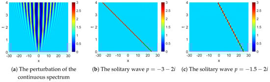
Figure 10. The numerical simulations of the perturbations and solitary waves.

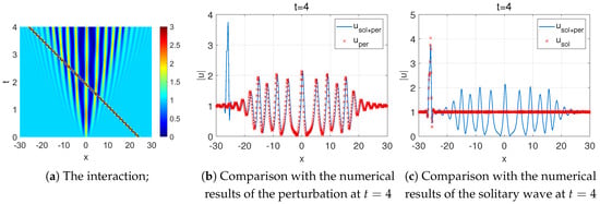
Figure 11. The numerical results for $p=-3-2i$.

In contrast for $p=-1.5-2i$, Figure 12a shows the case where the solitary wave propagates slower than the perturbation. After the solitary wave enters the region, the perturbation changes amplitude. Figure 12b shows a comparison with that of the disturbance at $t=4$. As stated in Theorem 2, the amplitude on the left side of the solitary wave reproduces that of the perturbation without any interaction. However, the amplitude profile on the right side of the solitary wave only roughly reproduces the shape of the perturbation. Both have undergone some minor translations. Figure 12c shows a comparison between the numerical simulation results of the interaction and those of the solitary wave. The speed of the solitary wave becomes slower because the asymptotic behavior is divided by ${\tilde{v}}_s$ when $p\in D_2^{+}$, indicating that the velocity of the solitary wave is converted to ${\tilde{v}}_s$ after entering the perturbation.

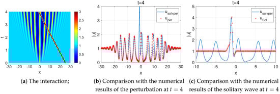
Figure 12. The numerical results for $p=-1.5-2i$.

Figure 13 shows the difference between the numerical results of the interaction and those of the perturbation. In these two situations, there is no difference between the part of the perturbation which is faster than the solitary wave and the solitary wave. As Theorems 1 and 2 describe, this part of perturbation is not affected. It has neither phase offset nor amplitude offset in space.

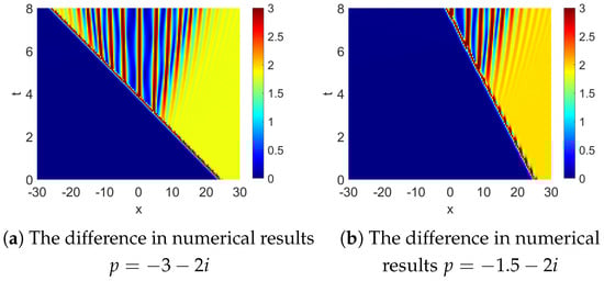
Figure 13. The difference in numerical results $|u_{sol+per}-u_{per}|$.

7. Discussions

This paper sheds light on the asymptotic behavior of solutions to the nonlinear Schrödinger equation in the presence of both the continuous spectrum and the second-order discrete spectra. By employing the Deift–Zhou nonlinear steepest descent method, we analyze the Riemann–Hilbert problem in the context of inverse scattering transform and examine the asymptotic behavior of the time terms in different regions of the complex plane. The paper presents a series of deformations to eliminate the time terms that tend to infinity along the curves in the Riemann–Hilbert problem. Through Laurent series expansions, the conditions during the deformation process are divided, and an appropriate deformation method is proposed to mitigate the divergent time terms.

In the end, the asymptotic behavior of the Riemann–Hilbert problem is characterized, indicating that when those appear both the perturbation corresponding to the continuous spectrum and solitary wave solutions corresponding to the second-order discrete spectra, the speed of the solitary wave remains unaffected if it is faster than the propagation speed of the perturbation. In this case, the phase of the perturbation undergoes a fixed offset, and its amplitude experiences spatial translation. On the other hand, if the speed of the solitary wave is slower than that of the perturbation, its velocity slightly decreases. Disturbances propagating faster than the solitary wave remain unchanged, while those propagating slower than the solitary wave undergo a fixed phase shift and spatial amplitude translation.

Finally, numerical experiments validate the conclusions presented in Theorems 1 and 2.

References

- Gardner, C.S.; Greene, J.M.; Kruskal, M.D.; Miura, R.M. Method for solving the Korteweg-de Vries equation. Phys. Rev. Lett. 1967, 19, 1095. [Google Scholar] [CrossRef]
- Shabat, A.; Zakharov, V. Exact theory of two-dimensional self-focusing and one-dimensional self-modulation of waves in nonlinear media. Sov. J. Exp. Theor. Phys. 1972, 34, 62. [Google Scholar]
- Ablowitz, M.J.; Segur, H. Solitons and the Inverse Scattering Transform; Society for Industrial and Applied Mathematics: Philadelphia, PA, USA, 1981. [Google Scholar]
- Yang, J. Nonlinear Waves in Integrable and Non-integrable Systems; Society for Industrial and Applied Mathematics: Philadelphia, PA, USA, 2010. [Google Scholar]
- Novikov, S.; Manakov, S.V.; Pitaevskii, L.P.; Zakharov, V.E. Theory of Solitions: The Inverse Scattering Method; Springer Science & Business Media: Berlin, Germany, 1984. [Google Scholar]
- Segur, H.; Ablowitz, M.J. Asymptotic solutions and conservation laws for the nonlinear Schrödinger equation II. J. Math. Phys. 1976, 17, 710–713. [Google Scholar] [CrossRef]
- Zakharov, V.; Manakov, S. Asymptotic behavior of non-linear wave systems integrated by the inverse scattering method. Sov. J. Exp. Theor. Phys. 1976, 44, 106. [Google Scholar]
- Deift, P.; Zhou, X. A steepest descent method for oscillatory Riemann-Hilbert problems. Bull. Am. Math. Soc. 1992, 26, 119–123. [Google Scholar] [CrossRef]
- Deift, P.; Venakides, S.; Zhou, X. The collisionless shock region for the long-time behavior of solutions of the KdV equation. Commun. Pure Appl. Math. 1994, 47, 199–206. [Google Scholar] [CrossRef]
- Kamvissis, S. On the long time behavior of the doubly infinite Toda lattice under initial data decaying at infinity. Commun. Math. Phys. 1993, 153, 479–519. [Google Scholar] [CrossRef]
- Deift, P.; Zhou, X. Long-time behavior of the non-focusing nonlinear Schrödinger equation, a case study. New Ser. Lect. Math. Sci. 1994, 5, 61. [Google Scholar]
- Buckingham, R.; Venakides, S. Long-time asymptotics of the nonlinear Schrödinger equation shock problem. Commun. Pure Appl. Math. 2007, 60, 1349–1414. [Google Scholar] [CrossRef]
- DE Monvel, A.B.; Kotlyarov, V.P.; Shepelsky, D. Focusing NLS equation: Long-time dynamics of step-like initial data. Int. Math. Res. Not. 2011, 2011, 1613–1653. [Google Scholar] [CrossRef]
- Jenkins, R.; Liu, J.; Perry, P.; Sulem, C. Soliton resolution for the derivative nonlinear Schrödinger equation. Commun. Math. Phys. 2018, 363, 1003–1049. [Google Scholar] [CrossRef]
- Yang, Y.; Fan, E. Soliton resolution for the short-pulse equation. J. Differ. Equ. 2021, 280, 644–689. [Google Scholar] [CrossRef]
- Biondini, G.; Mantzavinos, D. Long-time asymptotics for the focusing nonlinear Schrödinger equation with nonzero boundary conditions at infinity and asymptotic stage of modulational instability. Commun. Pure Appl. Math. 2017, 70, 2300–2365. [Google Scholar] [CrossRef]
- Pichler, M.; Biondini, G. On the focusing non-linear Schrödinger equation with non-zero boundary conditions and double poles. IMA J. Appl. Math. 2017, 82, 131–151. [Google Scholar] [CrossRef]
- Biondini, G.; Li, S.; Mantzavinos, D. Long-time asymptotics for the focusing nonlinear Schrödinger equation with nonzero boundary conditions in the presence of a discrete spectrum. Commun. Math. Phys. 2021, 382, 1495–1577. [Google Scholar] [CrossRef]
- Biondini, G.; Kovačič, G. Inverse scattering transform for the focusing nonlinear Schrödinger equation with nonzero boundary conditions. J. Math. Phys. 2014, 55, 031506. [Google Scholar] [CrossRef]
- Cox, S.M.; Matthews, P.C. Exponential time differencing for stiff systems. J. Comput. Phys. 2002, 176, 430–455. [Google Scholar] [CrossRef]
- Zheng, C.; Tang, S. Transparent boundary condition for simulating rogue wave solutions in the nonlinear Schrödinger equation. Phys. Rev. E 2022, 106, 055302. [Google Scholar] [CrossRef] [PubMed]
- Biondini, G.; Mantzavinos, D. Universal nature of the nonlinear stage of modulational instability. Phys. Rev. Lett. 2016, 116, 043902. [Google Scholar] [CrossRef] [PubMed]
Disclaimer/Publisher’s Note: The statements, opinions and data contained in all publications are solely those of the individual author(s) and contributor(s) and not of MDPI and/or the editor(s). MDPI and/or the editor(s) disclaim responsibility for any injury to people or property resulting from any ideas, methods, instructions or products referred to in the content. |
© 2025 by the authors. Licensee MDPI, Basel, Switzerland. This article is an open access article distributed under the terms and conditions of the Creative Commons Attribution (CC BY) license (https://creativecommons.org/licenses/by/4.0/).