Abstract
In this paper, an integrated geometric and thermal-induced errors prediction approach for active error compensation in machine tools is proposed and evaluated. The proposed approach is based on a hybrid of physical and neural network predictive modeling to drive an adaptive position controller for real-time error compensation including geometric and thermal-induced errors. Error components are formulated as a three-dimensional error field in the time-space domain. This approach involves four key steps for its development and implementation: (i) simplified experimental procedure combining a multicomponent laser interferometer measurement system and sixteen thermal sensors for error components measurement, (ii) artificial neural network-based predictive modeling of both position-dependent and position-independent error components, (iii) tridimensional volumetric error mapping using rigid body kinematics, and finally (iv) implementation of the real-time error compensation. Assessed on a turning center, the proposed approach conducts a significant improvement of the machine accuracy. The maximum error is reduced from 30 µm to less than 3 µm under thermally varying conditions.
1. Introduction
The growing demand for enhanced dimensional accuracy in machining processes creates the need to develop cost-effective and efficient methods to improve the performance of CNC machines tools (MT). Dimensional accuracy is one of the most crucial factors in determining this performance. Typically, errors affecting MT are defined as the deviations between the real and measured positions and orientations of the cutting tool with respect to a reference system associated with the machined part. Most recent MT are equipped with a positioning resolution of 1 µm. Under challenging machining conditions—such as prolonged operation, thermal fluctuations, or hard material cutting—machine accuracy can degrade significantly, leading to notable deviations in dimensional accuracy. To maintain the MT performances at acceptable levels, these deviations need to be detected, identified, and removed. Modern CNC systems provide a foundation for such correction through software-based compensation mechanisms, often using geometric models such as the Homogeneous Transformation Matrix (HTM) framework. Based on principles such as those of Abbé and Bryan, these models enable systematic correction of geometric errors, aligning measurement systems with motion or mathematically accounting for angular deviations when direct alignment is impractical [1,2,3].
Machine tools are affected by various sources of error, including geometric [4,5], thermal-induced [6], dynamic [7,8], structural [9], and assembly-related deviations [10,11]. Geometric and thermal-induced errors are responsible for a substantial portion of the observed inaccuracies, accounting for approximately 70% of the total volumetric error [12]. These two categories, which vary gradually over time, are associated with inherent geometric imperfections resulting from manufacturing defects, misalignments during assembly and installation, as well as thermally driven distortions caused by internal and external heat sources [13]. Other error sources include dynamic deviations generated by spindle movement, cutting force variations, and inertial-induced deflections. Although their individual effects may be comparatively limited, the influence of these errors remains significant due to their interactions with primary error sources. Moreover, while certain errors directly impact machining accuracy, others manifest through coupled mechanisms, producing variable, active, and difficult-to-predict deviations. Consequently, the characterization and mitigation of these error sources have been the focus of extensive research efforts aimed at enhancing dimensional precision and performance in advanced manufacturing systems.
Historically, error mitigation in CNC machine tools relied on structural improvements to enhance geometric and thermal stability, but this approach becomes prohibitively expensive as precision demands increase. Modern strategies now focus on compensation-based methods, which are more cost-effective and adaptable [14]. These are broadly divided into suppression and active compensation techniques. Suppression methods reduce thermal effects through coolant systems, thermally stable materials, or thermal balancing, yet they often raise system complexity and remain limited under variable operational conditions [15]. In contrast, active compensation employs physical or data-driven models to predict and correct thermal deformation in real time [16]. This requires the optimal selection of temperature-sensitive points (TSPs), identified using finite element analysis, statistical correlation, or machine learning algorithms [15]. Recent advancements emphasize sensor integration and predictive control to sustain machining accuracy without altering machine structure.
Recent studies have proposed a range of predictive models to improve thermal compensation in CNC machining systems. These methods aim to predict and correct thermally induced deviations to sustain dimensional accuracy during operation [17]. Statistical modeling approaches—such as Least Squares, Multivariable Regression, and gray System Theory—provide interpretable and efficient solutions for basic thermal behavior but often fall short under complex or nonlinear conditions [18]. For instance, Shi et al. [19] applied multiple linear regression to model origin and position-related thermal errors in CNC lathes, achieving a 92.5% reduction in positioning error, while Liu et al. [20] improved model robustness by combining ridge regression and principal component regression with temperature interval segmentation. Mareš et al. [21] employed transfer function modeling, calibrated through thermal cycling experiments, and implemented real-time compensation via embedded Python scripts. However, the adaptability of these methods remains limited under highly nonlinear, time-varying, or data-sparse operating conditions.
To address these limitations, data-driven and AI-integrated techniques have been extensively explored. Machine learning approaches—such as Support Vector Machines, Gaussian Process Regression (GPR), and ensemble methods like XGBoost—demonstrate enhanced modeling capacity and resilience. Wei et al. [22] proposed a novel GPR-based thermal error modeling and compensation framework for CNC machine tools, which incorporates interval prediction to reflect the stochastic nature of thermal behavior and introduces an adaptive mechanism for selecting temperature-sensitive points (TSPs) during model training. Their method, validated on a three-axis vertical machining center, significantly outperformed conventional techniques—including Ridge Regression, Principal Component Regression, ARX, and LSTM—in both accuracy and robustness, and achieved substantial reductions in thermal and angular machining errors during real-time compensation experiments. Similarly, Ye et al. [23] developed the ALIX model, which integrates adaptive LASSO with XGBoost to improve prediction accuracy and variable interpretability. Assessed on 23 experimental batches from a Vcenter-55 vertical machining center, ALIX outperformed baseline models such as OLS, LASSO-SVM, and Random Forests in terms of prediction robustness, worst-case deviation, and percentage error. Real-time validation confirmed ALIX’s capacity to maintain thermal deviation within 10 µm under varying operating conditions, thereby demonstrating its practical utility in industrial settings. Neural networks further broaden this landscape. Farias et al. [24] implemented a radial basis function neural network directly into the programmable logic controller of a legacy three-axis CNC milling machine. Trained on temperature data from six RTD sensors and axis position feedback, the model achieved up to 77.8% error reduction on the Y-axis during real-time operation, validated on 1080 distinct data points, and offered a cost-effective, retrofittable solution for older systems. Shen et al. [25] introduced an intelligent CNC control scheme featuring a back-propagation neural network (BPNN) with adaptive learning, integrated with an Online Temperature Measurement System (OTMS). Using gray correlation analysis to associate temperature variation with thermal deformation, the model enabled dynamic error compensation. Deployed on a Leaderway V-450 machine, the system outperformed traditional predictors in both convergence speed and accuracy, with OTMS providing over 95% temperature measurement accuracy within 2 s. The enhanced TECM achieved a minimum contour machining error of 0.02 × 10⁻³ mm, confirming its efficacy in improving thermal precision and aligning with intelligent manufacturing paradigms.
Recent work has also advanced deep learning architecture and intelligent control frameworks. Nguyen et al. [26] developed a Long Short-Term Memory (LSTM) neural network using data from 32 PT-100 temperature sensors, applying Pearson correlation to identify the seven most influential temperature points. This enabled accurate prediction of thermal errors across X, Y, and Z axes, with real-time compensation reducing errors from 7 µm to 3 µm in X, 74 µm to 21 µm in Y, and −64 µm to −20 µm in Z. Du et al. [27] proposed a 12-layer Convolutional Neural Network (CNN) that processes raw temperature data converted into thermal images, eliminating manual temperature-sensitive point selection and integrating depthwise separable convolutions and dropout regularization to optimize computational efficiency. Embedded in an STM32F4 microprocessor, this system achieved an 80% reduction in radial thermal error on a CNC grinder, lowering error from 35 µm to 7 µm. Zimmermann et al. [28] introduced the Thermal Adaptive Learning Control (TALC) framework, which combines phenomenological models with one-class Support Vector Machines (SVMs) for novelty detection, enabling autonomous, on-demand thermal state measurements. TALC reduced state-triggered measurement updates by 78%, increased machine productivity by 3%, and maintained high compensation accuracy during 5-axis machining. Li et al. [29] proposed the Unit Adaptive Thermal Network (UATN), a model dynamically adjusting thermal units to capture stochastic, time-varying thermal behaviors. Integrating thermal imager and thermocouple data with machine state parameters, the UATN compensates axial thermal deformation in feed screw and spindle systems, achieving sub-micrometer accuracy and stable performance under variable conditions Huang et al. [30] developed a dynamic compensation strategy integrating multiple thermal models within an embedded control architecture on a VMC655H vertical machining center. Utilizing Kalman filtering, clustering, and gray correlation analysis for temperature-sensitive point selection, their method achieved a 53.11% improvement in X-axis positioning accuracy, effectively mitigating thermal deformation, and maintaining machining precision under varying conditions. Also, studies have explored advanced data-driven approaches, including attention-based LSTM networks for predictive modeling under complex conditions and generalized errors-in-variables models for pose estimation, highlighting the ongoing development of intelligent compensation systems [31,32].
Despite notable advancements, current compensation models exhibit key limitations that restrict their deployment in industrial scenarios. Statistical methods are often constrained by their linear assumptions and lack of robustness under dynamic thermal conditions. AI-based models, while more adaptable, frequently overlook the physical structure of machine behavior and are difficult to interpret. Moreover, most compensation strategies either target uniaxial errors or function offline, limiting their responsiveness and real-world applicability. To bridge this gap, the present study proposes a real-time compensation strategy for geometric and thermally induced errors based on a simplified experimental approach integrated with simultaneous and dynamic prediction of error components. These components are categorized into position-dependent and position-independent errors: the former are modeled as a function of both nominal axis positions and temperatures at multiple locations, while the latter are driven solely by thermal inputs. At each sampling instance, total volumetric errors are computed using a hybrid model that integrates a physically grounded HTM with a neural network predictor. This dual-layered framework enables interpretable, accurate, and real-time error correction, directly implemented within the CNC control loop.
2. Modeling Techniques for Geometric-Thermal Volumetric Error
In typical MT, the volumetric error is defined as the error vector resulting from the combination of individual errors in the machine workspace. Figure 1 illustrates this error at the tip of the cutting tool for a two-axis turning center. To evaluate the components of the volumetric error, the ideal solution consists of directly measuring the deviation associated with the geometric and thermal errors under explicit machine thermal conditions with respect to a specific reference. However, this solution is compromised by the lack of reliable instrumentation for direct measurements. An alternative approach consists of combining geometric and thermal errors in the same measurement. With this in mind, two classes of error components can be identified: position-dependent and position-independent error components.

Figure 1.
Ideal and actual position of cutting tool relative to workpiece.
2.1. Modeling of Position-Dependent Error Components
The modeling of the position-dependent error components is usually more complicated than the modeling of the position-independent error components because this type of error is not only a function of the positions but also a function of the temperature field. Fortunately, these error components can be considered as the combination of geometric errors and the variation in the geometric errors under the effects of the MT thermal conditions.
The geometric errors are related to the mechanical imperfections in the MT structure resulting from manufacturing defects and misalignments due to assembly and installation. Geometric inaccuracies produce various linear and angular error components between the moving elements of the machine. This results in errors in position and orientation errors of the cutting tool with respect to the workpiece. Figure 2 illustrates a schematic representation of the six error components associated with a linear axis of a machine tool. The symbols used in the figure are presented in Table 1 where εij represents angular error motions, with i representing the axis the motion rotates about, and j representing the intended motion direction. The positive rotation is defined by the right-hand rule. δij represents the translational error in direction i during the motion in direction j.

Figure 2.
Schematic representation of six degrees of freedom error motion of a machine tool carriage system.

Table 1.
Error categorization in a machine tool axis.
Multi-axis machine tools are composed of a sequence of linkages connected by joints, providing either rotational or translational motion. By applying rigid body kinematics, the relative position of each axis of an MT with respect to each other and with a global reference frame can be described using a homogeneous transformation matrix (HTM), which is a 4 × 4 matrix in 3-dimensional space. An HTM can represent a coordinate system with respect to another or a reference coordinate system. The HTM expresses the pure translation of an ideal carriage for the X-axis in the following form:
where x refers to the position of the X-axis coordinate system (Ox, Xx, Yx, Zx) with respect to the reference coordinate system (O, X, Y, Z). When using the six degrees of freedom error motion, the total axis error is characterized by a combination of rotational and translational components. Using HTM and assuming small angular deviations, the actual translation along a real X-axis is given by:
The positioning error is defined as the deviation between the actual and the desired tool position. The actual position can be derived by multiplying successively all the actual HTMs. The schematic representation of the coordinate frame assignments on a turning center is illustrated in Figure 3.
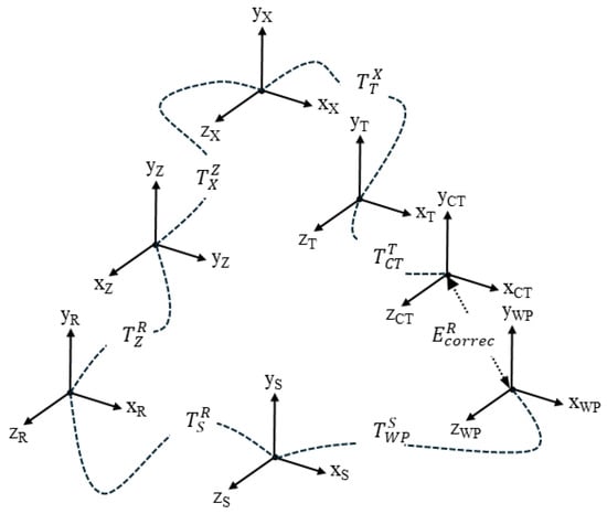
Figure 3.
Schematic representation of coordinate frame assignments on a turning center.
The HTM that describes the spatial relationship between the reference coordinate system (R) and the cutting tool coordinate system (CT) is expressed by Equation (3). The relationship between the reference coordinate system (R) and the workpiece coordinate system (WP) is expressed by Equation (4).
where X and Z are the MT axis, S is spindle, and T is the turret.
and are represented by the following vectors in their respective coordinate frames.
Since all these linkages are not perfect, this will cause a relative error between cutting tool and workpiece. Therefore, the actual spatial relationship between the cutting tool and a given point on the workpiece can be expressed as:
where E is the volumetric error homogenous transformation matrix representing position and orientation errors between the cutting tool and workpiece. The position vector components of E represent the translations that must be made to be at the appropriate location on the workpiece. To move the axes to the desired location, inverse kinematic solutions should be used. Since there are only translational axes, volumetric errors, E can be calculated using exclusively the position vectors of the HTM. The error correction vector with respect to the reference coordinate system can be obtained from the following equation.
where, Ecx, Ecy and Ecz are the volumetric error compensation components in the X, Y and Z directions, respectively.
Because of Abbe offsets and angular orientation errors of the axes, will not necessarily be equal to the position vector component of E. However, does represent the incremental motions of X and Z axes to compensate for cutting tool tip position errors. The expanded form of (9) is obtained as follows:
where X and Z are the nominal machine positions, WPx and WPz are obtained from workpiece geometry, CTx, CTy and CTz are obtained from cutting tool geometry, δxOD and δzOD are the thermal drifts at the origin of the machine axes, δxWP and δxWP are functions of thermal and static load deformations, δxS, δzS and εyS are spindle thermal drift characteristics, and δxCT and δzCT are functions of thermal and load deformation and wear. δxT, δzT and εyT are functions of angular position of the turret, δxx, δzx, δxz, εyx, δzz, εyz are functions of machine geometry, the position along the axes and machine thermal conditions.
Ecx = δxOD − δxx − δxz + δxWP + δxS − δxT − δxCT + WPx − X − CTx − CTz × (εyz + εyx + εyT) + (WPz × εyS)
Ecy = δzOD − δzx − δzz + δzWP + δzS − δzT − δzCT + WPz − Z − CTz + CTx × (εyz + εyx + εyT) + (X × εyz) − (WPx × εyS)
Considering the machine geometric configuration, that there is no relative movement of the turret with respect to the X axis and that there is no machining and therefore no load, it is possible to adopt the following assumption.
WPx − CTx − X = 0 and WPz − CTz − Z = 0.
δxT = δzT = εyT = 0.
δxCT = δzCT = δxWP = δzWP = 0
As a result, Equations (10) and (11) can be simplified in the form of Equations (15) and (16).
Ecx = δxOD − δxx − δxz + δxS − CTz ∗ (εyz + εyx) + (WPz ∗ εyS)
Ecz = δzOD − δzx − δzz + δzS + CTx ∗ (εyz + εyx) + (X ∗ εyz) − (WPx ∗ εyS)
From Equations (15) and (16) it is easy to identify eight position-dependent error components including four translational (δxx, δxz, δzx and δzz) and two rotational errors (εyx and εyz). Because this type of error is not only a function of the positions but also a function of the temperature field, it can be estimated using artificial neural network (ANN) models. The interest of ANNs lie in their capacity to model and generalize without overfitting highly nonlinear relationships. This is very useful to reduce the measurement and the off-line calibration efforts.
2.2. Modeling of Position-Independent Error Components
The modeling approach incorporates two groups of position-independent error components. These errors are influenced solely by the machine’s temperature field, coordinate system thermal drift, and spindle thermal drift. Assuming linear effects, the coordinate system thermal drift (δxOD and δyOD) due to machine tool (MT) thermal disturbances can be represented as an error vector, which is estimated under various thermal states of the machine and must be added to the volumetric error components vector. In a turning center, three spindle thermal drift components are critical for maintaining machine accuracy: axial thermal drift (δzs), which causes displacement along the Z-axis; radial thermal drift (δxs), which occurs perpendicular to the Z-axis; and tilt thermal drift (εys), which reflects an angular deviation of the spindle axis within the X–Z plane. Although various empirical techniques can be employed to model position-independent error components, artificial neural networks have been chosen for modeling these errors.
3. Model Building and Simulation
To develop an effective prediction model for geometric and thermal-induced errors aimed at active error compensation, error components are categorized into three groups based on similar characteristics, measurement procedures, and instrumentation. These groups include thermal drift at the origins of the machine tool (MT) axes, position-dependent error components, and spindle thermal drift. Specialized devices are necessary to measure temperature variations at various locations within the MT structure, simultaneously capturing the thermal deformation reflected in the positioning errors of the spindle and along the machine axes.
While the HTM-based formulation provides a complete and interpretable physical model of the geometric and thermal errors, the real-time application of such a model requires the continuous estimation of multiple error components that are highly nonlinear, time-dependent, and sensitive to thermal dynamics. Direct measurement of these components is often impractical, and analytical modeling under variable thermal states becomes computationally intensive. To address this challenge, we adopt a hybrid approach where individual error components are estimated in real time using ANNs. These data-driven models are trained to learn the complex relationships between machine positions, temperature sensor inputs, and error behaviors. The predicted error components are then integrated back into the HTM-based volumetric error equations to compute real-time compensation values. This hybrid structure preserves the physical interpretability of the kinematic framework while leveraging the predictive strength and adaptability of neural networks.
3.1. Measurement of Error Components
As illustrated in Figure 4, the used devices for error components measurement are: (i) 16 thermistors with measuring range from −20 °C to 120 °C and resolution of 0.0625 °C to track the temperature distribution in the most sensitive areas of the MT (ii) an API XD laser interferometer system to assess the positioning error in X and Z directions, in accordance with the ISO230-2 standard [33], and the machine axes origins thermal drifts, and (iii) a simplified five displacement traditional non-contact sensors method to evaluate the spindle thermal drifts (two transitional drifts and angular inclination of the spindle axis), according to the ISO230-3 standard [34]. Temperatures and various geometric and thermal error components must be measured concurrently to ensure that each set of thermal errors corresponds to a specific temperature distribution.
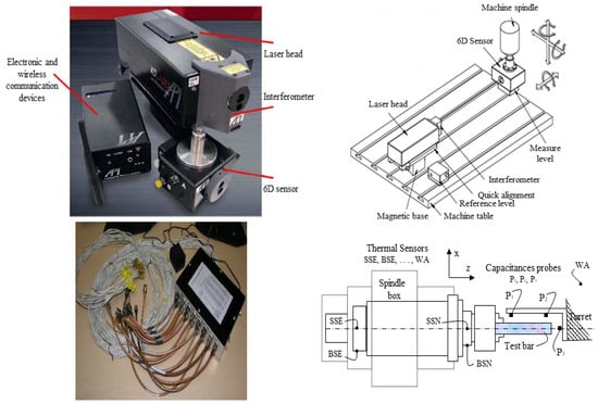
Figure 4.
Temperature and thermal error measurement.
Thermal sensor location is crucial in any thermal error modeling and compensation strategy. If possible, the temperature sensors must be located near the structural elements which endure most of the thermal distortions. In this case, 16 thermistors are carefully positioned to track the temperature distribution in the most sensitive areas of the MT. Preliminary experimental investigation results suggest that some machine components only have small temperature variations, and the temperature variation in other components are not consistently interrelated to the thermally induced errors. The experimental exploration also indicates a powerful connection between average temperature growth along the spindle axis and thermal errors, which is strongly correlated to the spindle speed. Therefore, only 10 temperature sensor locations are retained as relevant variables to investigate in this application. The proposed locations are explicitly identified in Table 2.
Table 2.
Identification of temperature sensor locations.
Environmental temperature fluctuations can result in an increase in thermally induced errors. It is therefore necessary to evaluate the effects of time-varying environmental temperature on the growth of thermal errors. For this purpose, some samples of environmental temperature and thermal error are collected for 24 h without machine operation. The results reveal that the effect of environmental temperature is small (1 to 2 µm). The correlation between the temperature and thermal errors is insignificant (less than 1%). This is attributed to the irregular growth of thermal drifts within a typical temperature range. Therefore, the contribution of environmental temperature to thermal error variation can be considered negligible. To characterize the thermally induced changes in the machine errors, the measurements are taken over representative temperature spectrum of the machine. Figure 5 shows a typical temperature evolution, where the MT operates at specific federate speed and spindle rotation speed for 4 h, then stops for 4 h. This figure shows a clear distinction between the average temperature around the spindle (31 °C) and the temperature along the axes (26 °C). It can be observed also that the maximum temperature around the spindle is recorded at the bottom of the spindle end. Along the axes, the maximum temperature is recorded at the backside of X-slide drive mechanism, nevertheless the difference with the other locations around does not exceed 1 °C. During similar warm-up and cold-down cycle, the observed thermal expansion of the MT frame expressed in the form of machine axes origins thermal drifts error is illustrated in Figure 6.
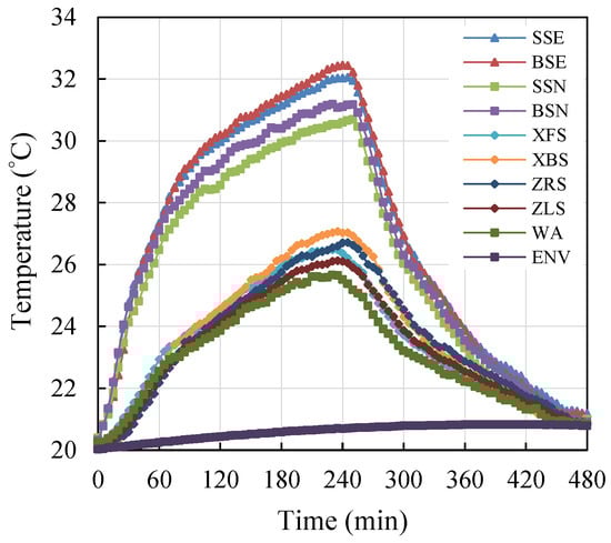
Figure 5.
Typical temperature profile of the machine elements measured under warm-up and cool-down conditions.
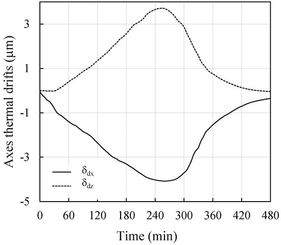
Figure 6.
Axes origins thermal drifts error.
Measurements of positioning error in X and Z directions are carried out at displacement intervals of 20 and 30 mm, respectively. Results of the geometrical error measurements at a temperature of 20 °C approximately, illustrated in Figure 7, show that the linear displacement error of the X-axis (more than 8 µm for a 300 mm travel) and the Z-axis (more than 18 µm for a 450 mm travel) are larger than the specified MT accuracy of ±5 µm. The straightness errors vary within intervals 3–6 and 2–5.5 µm, respectively, over X and Z directions. The angular errors measured at the same positions and the same thermal conditions are similarly presented. The angular errors vary within intervals 2–6 arcsec and 1–3 arcsec, respectively, over X and Z directions.
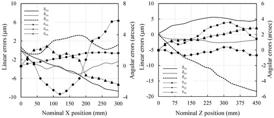
Figure 7.
The X and Z displacement error measured at about 20 °C.
Observations from error measurement under mixed thermal conditions show that although errors varied with the average temperature, their basic appearances along the axes did not fundamentally change, as shown in Figure 8. This observation concerns both translational errors and angular errors. The position-dependent errors can be expressed as the summation of the stationary parts (geometric errors) and time-variant parts. The stationary errors are active under cold machine starting conditions. During the machine operation, the time-variant errors (thermally induced errors) are added to the geometric errors.
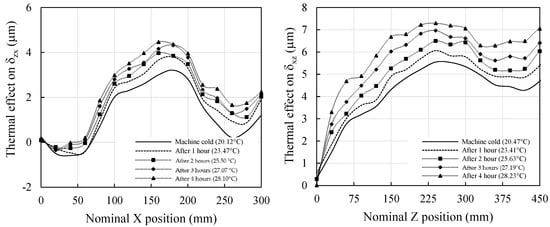
Figure 8.
Example of errors variation as a function of position and machine thermal conditions.
Three initial investigations reveal a strong relationship between spindle thermal drifts and the rise in the average temperature increase along the spindle, as well as the spindle speed. For the spindle thermal drifts measurement (two transitional drifts and angular inclination of the spindle axis), the spindle rotates at selected rotating speeds for 4 h and then remains stopped for 4 h. During this time, the spindle thermal drifts and the temperature history are continuously monitored. The results outlined in Figure 9 show that the thermal drifts and the average temperature profiles do not increase proportionally with the speeds. However, it is noteworthy that the growth of thermal drifts closely follows the variations in temperature. This characteristic offers significance in the modeling process providing the option to avoid including the spindle rotation speed as a variable in the prediction model.
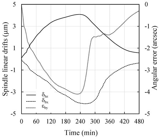
Figure 9.
Spindle thermal drifts variation under warm-up and cool-down machine thermal conditions.
3.2. Error Modeling and Simulation
The prediction of the resultant error components (Ecx and Ecz) at any location in the machine workspace and any machine thermal conditions requires the prediction of all the error components identified in Equations (16) and (17). The position-dependent error components are considered as a combination of axis nominal positions and temperatures at various locations. The position-independent error components depend only on temperatures at various locations. Considering that, four ANNs models are needed to predict all the error components (X-axis, Z-axis, coordinate system thermal drift and spindle thermal drift). The algorithmic framework to implement these models is schematically illustrated in Figure 10. The nominal positions of the machine slides and the temperature sensors installed on the MT structure are scanned at a constant sampling rate. For every sample, each error component is predicted using the appropriate ANN model and integrated via Equations (16) and (17) for the prediction of the resultant error components.
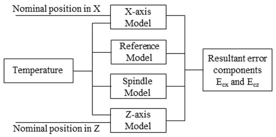
Figure 10.
A schematic representation of the ANNs model integration.
The hybrid modeling framework integrates the HTM approach with data-driven ANN predictions to compute the total volumetric errors. The ANN models are trained to predict individual error components—both position-dependent and position-independent—using machine axis positions and temperature inputs. Once these individual components are estimated by the ANN models in real time, they are substituted into the HTM-based equations (Equations (16) and (17)), which represent the analytical formulation of the volumetric error vectors Ecx and Ecz. The HTM framework functions as a structured kinematic model that synthesizes the ANN outputs into physically meaningful error correction vectors. These vectors are then applied via the CNC’s compensation interface to correct the actual tool tip position.
The X-axis ANN model is based on the X position and four temperature sensors (XFS, XBS, ENV and WA) as inputs and error components (δxx, δyx, δzx, and εxx, εyx, εyx) as outputs while the Z-axis ANN model is based on the Z position and four temperature sensors (ZRS, ZLS, ENV and WA) as inputs and error components (δxz, δyz, δzz, and εxz, εyz, εyz) as outputs. The coordinate system drift model is built using XFS, XBS, ZRS, ZLS, ENV and WA as input and (δxOD and δzOD) as outputs. The spindle drift model uses SSN, BSN, SSE, BSE, ENV and WA as inputs and δzs, δxs, and εys as outputs.
To assess the performance of the proposed ANN models, many statistical measures such as Mean absolute deviation (MAD), Mean absolute percent error (MAPE), Root mean square error (RMSE) and Coefficient of determination R2 are adopted. These metrics are explicitly expressed in Equations (17)–(20).
The performances of the four models are particularly good and present an important advantage for predicting the resultant error components both in terms of precision and reliability as well as in terms of robustness. The summary of modeling performance is presented in Table 3. These results reveal that despite the intuitive choice of the temperature sensors included in each model, the quality of the predictions is beyond expectations. This confirms overall that each individual error component depends strongly on the temperature sensors distributed along its generative axis. A systematic procedure addressing the best selection of sensors to be considered in each model will be presented in a future paper.
Table 3.
ANN modeling performance summary.
Once the four predictive models are established, the compensation values Ecx and Ecz are synthesized using the algorithm illustrated in Figure 10. The simulation tests conducted for various MT thermal conditions indicate the effectiveness of the adopted prediction approach. Figure 11 illustrates the spatial-variant error components at environmental temperature (average temperature of 20.27 °C) and the difference between measured and predicted resultant error components in the X-Z-plane. It can be seen that the model fits very well the geometric position-dependent error components. Maximum errors without compensation reached 13 µm in the x-direction and 23 µm in the Z-direction. The residual errors show that the error can be reduced to within a 3 µm range after compensation. Figure 12 and Figure 13 illustrate the spatial-variant error components and compare measured and predicted errors in the X-Z-plane at average temperatures of 23.31 and 26.23 °C, respectively. In these two cases, maximum errors without compensation varied around 15 µm in the x-direction and around 28 µm in the Z-direction. The residual errors are reduced to less than 4 µm range after compensation. The quality of the prediction of the geometric-thermal errors is also confirmed at arbitrary average temperature between 20 and 30 °C. The predictive modeling approach provided a good prediction of the volumetric error under various machine thermal conditions, with an average error less than 4 µm.

Figure 11.
Measured errors (MEx and MEz), predicted errors (PEx and PEz) and Residual errors (REx and REz) in the X and Z-directions at an average temperature of 20.27 °C.
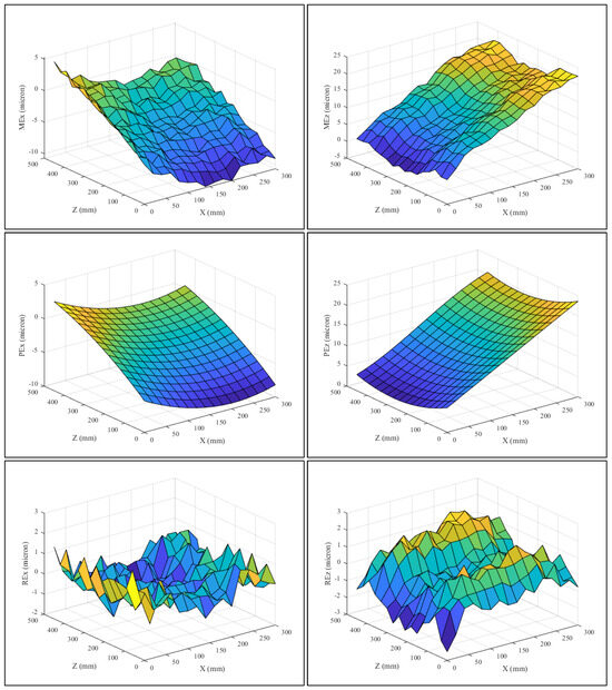
Figure 12.
Measured errors (MEx and MEz), predicted errors (PEx and PEz) and residual errors (REx and REz) in the X and Z-directions at an average temperature of 23.31 °C.
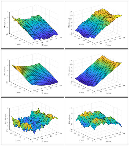
Figure 13.
Measured errors (MEx and MEz), predicted errors (PEx and PEz) and residual errors (REx and REz) in the X and Z-directions at an average temperature of 26.23 °C.
Table 4 summarizes the statistical tests conducted to evaluate the predictive model’s accuracy for the two resultant error components (Ex and Ez) according to three different thermal cycles. Results show that the model performs very well. Despite maximum deviations reaching 15 µm in X and 28 µm in Z, the model maintains a mean absolute deviation below 1 µm, a mean absolute percentage error under 15%, and a small root mean square error. Coefficients of determination (R2) range from 94% to 98% depending on the axis. Performance at 20.27 °C slightly exceeds that at 23.31 °C and 26.23 °C, suggesting minor challenges in capturing temperature-induced errors. Overall, predictive accuracy remains high enough to effectively drive error compensation.
Table 4.
ANN modeling performance summary.
To assess the actual performance of the model and its predictive accuracy under operating conditions not included in the training and testing datasets, additional tests are conducted under new thermal cycles. Since it is not possible to conduct the experiments with and without compensation using a single test, two separate tests are performed: one without compensation and the other with compensation. For this evaluation, an external error compensation system is implemented using the “external mechanical origin offset” function available in CNC systems. This method avoids modifications to CNC commands, ensuring that the workpiece coordinates would not be influenced.
The proposed evaluation procedure consists of assessing the model capacity during combined axis movements using the well-known diagonal test. Resultant error components, Ex and Ez, along the diagonals in the XZ plane, are derived from both measured and predicted error components under identical thermal conditions. Data are sampled at consistent intervals of 20 mm along the X-axis and 30 mm along the Z-axis. Throughout both tests, the average temperature remained relatively stable, fluctuating between 24.30 and 24.56 °C.
To evaluate the performance of the proposed predictive model, measured and predicted error components along selected diagonals are compared. Table 5 and Figure 14 present the results with and without compensation. These results demonstrate that the model maintains strong accuracy and robustness, even under varying temperature conditions. The residual errors are significantly reduced—from approximately 7 µm to less than 2.2 µm in the X direction, and from around 18 µm to below 4.5 µm in the Z direction—corresponding to accuracy improvements of 68% and 75%, respectively. This indicates the model’s effectiveness and confirms that the mapping between temperature variation and positioning errors remains consistent.
Table 5.
Comparison of positioning errors in X and Z directions before and after error compensation.
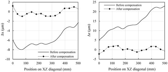
Figure 14.
Positioning errors in X and Z directions before and after error compensation.
Although this study focuses on a two-axis turning center, the proposed hybrid methodology is extendable to multi-axis machines. The HTM formulation is inherently scalable to additional kinematic chains, and the ANN models can be retrained to capture more complex error behavior in milling or 5-axis systems, given sufficient sensor data and calibration.
4. Conclusions
To meet the rising demand for higher-quality machined parts, enhancing the accuracy of CNC machine tools through error compensation has emerged as a key priority in modern manufacturing. The success of such an approach depends on the degree of accuracy, robustness, and reliability of the model to evaluate in real time the error components at any location in the machine workspace. Based on a hybrid of physical and neural network predictive modeling, the proposed approach makes it possible to drive an adaptive position controller for real-time error compensation of geometric and thermal-induced errors. Twenty-nine error components are considered in the modeling process. Among these error components, only eleven are important in this specific machine including six position-dependent errors in x and z directions and five position-independent errors as thermal drifts for spindle and for the origins of the machine axes. Sixteen temperature sensors are initially used to identify the temperature field in the machine. Finally, only 10 temperature sensor locations are retained as relevant variables to investigate in this application. Simplified experimental procedure combined with artificial neural network based predictive modeling and tridimensional of volumetric error mapping using rigid body kinematics are successfully achieved to produce the real-time error compensation values. Evaluated on a turning center, the proposed approach leads to a significant improvement of the machine accuracy. The maximum resultant error is reduced from 32 µm to less than 4 µm under thermally varying conditions.
This work represents a necessary first step in isolating and compensating thermally induced errors under controlled conditions. Future work will focus on validating the proposed model under real machining environments, including dynamic loads and cutting operations, to assess its robustness and extend its industrial applicability.
Author Contributions
Conceptualization, W.C. and A.E.O.; methodology, W.C. and A.E.O.; software, W.C. and A.E.O.; validation, W.C., A.E.O. and N.O.; formal analysis, W.C. and A.E.O.; investigation, W.C. and A.E.O.; resources, A.E.O.; data curation, W.C.; writing—original draft preparation, W.C., A.E.O. and N.O.; writing—review and editing, W.C., A.E.O. and N.O.; visualization, W.C., A.E.O. and N.O.; supervision, A.E.O. All authors have read and agreed to the published version of the manuscript.
Funding
This research received no external funding.
Data Availability Statement
The data that support the findings of this study are not publicly available but are available from the corresponding author upon reasonable request.
Conflicts of Interest
The authors declare no conflict of interest.
References
- Seid Ahmed, Y.; Amorim, F.L. Advances in computer numerical control geometric error compensation: Integrating AI and on-machine technologies for ultra-precision manufacturing. Machines 2025, 13, 140. [Google Scholar] [CrossRef]
- Bhattacharyya, A.; Schmitz, T.L.; Payne, S.W.T.; Choudhury, P.R.; Schueller, J.K. Introducing engineering undergraduates to CNC machine tool error compensation. Adv. Ind. Manuf. Eng. 2022, 5, 100089. [Google Scholar] [CrossRef]
- Ramesh, R.; Mannan, M.A.; Poo, A.N. Error compensation in machine tools—A review: Part I: Geometric, cutting-force induced and fixture-dependent errors. Int. J. Mach. Tools Manuf. 2000, 40, 1235–1256. [Google Scholar] [CrossRef]
- Tayier, W. Enhancing CNC precision: A review of geometric errors and simulation methods in three-axis CNC systems. J. Eng. Technol. Adv. 2024, 9, 55–74. [Google Scholar] [CrossRef]
- Lin, Z.; Tian, W.; Zhang, D.; Gao, W.; Wang, L. A method of geometric error identification and compensation of CNC machine tools based on volumetric diagonal error measurements. Int. J. Adv. Manuf. Technol. 2023, 124, 51–68. [Google Scholar] [CrossRef]
- Skrypnyk, T.; Korenkov, V. Temperature compensation in ball screws of CNC machines. Mech. Adv. Technol. 2025, 9, 157–165. [Google Scholar] [CrossRef]
- Lu, Y.; Fan, Y.; Zhao, J.; Liu, S.; Chen, N. Real-time arc length parameter-based integrated control strategy of contour error compensation for free-form curve CNC machining. Int. J. Adv. Manuf. Technol. 2024, 131, 1769–1794. [Google Scholar] [CrossRef]
- Jiang, Y.; Chen, J.; Zhou, H.; Yang, J.; Hu, P.; Wang, J. Contour error modeling and compensation of CNC machining based on deep learning and reinforcement learning. Int. J. Adv. Manuf. Technol. 2022, 118, 551–570. [Google Scholar] [CrossRef]
- Fu, X.; Song, H.; Li, S.; Lu, Y. Digital twin technology in modern machining: A comprehensive review of research on machining errors. J. Manuf. Syst. 2025, 79, 134–161. [Google Scholar] [CrossRef]
- He, W.; Zhang, L.; Hu, Y.; Zhou, Z.; Qiao, Y.; Yu, D. A Hybrid-Model-Based CNC Machining Trajectory Error Prediction and Compensation Method. Electronics 2024, 13, 1143. [Google Scholar] [CrossRef]
- Wang, S.-M.; Lee, C.-Y.; Gunawan, H.; Yeh, C.-C. On-line Error-Matching Measurement and Compensation Method for a Precision Machining Production Line. Int. J. Precis. Eng. Manuf.-Green Technol. 2022, 9, 493–505. [Google Scholar] [CrossRef]
- Gu, G.-W.; Park, M.-S.; Suh, J.-H.; Lee, H.-H. A Technique for Integrated Compensation of Geometric Errors and Thermal Errors to Improve Positional Accuracy of Hole Machining in Large-Size Parts. Int. J. Precis. Eng. Manuf. 2024, 25, 1541–1555. [Google Scholar] [CrossRef]
- Ramesh, R.; Mannan, M.A.; Poo, A.N. Error compensation in machine tools—A review: Part II: Thermal errors. Int. J. Mach. Tools Manuf. 2000, 40, 1257–1284. [Google Scholar] [CrossRef]
- Li, Y.; Zhao, W.; Lan, S.; Ni, J.; Wu, W.; Lu, B. A review on spindle thermal error compensation in machine tools. Int. J. Mach. Tools Manuf. 2015, 95, 20–38. [Google Scholar] [CrossRef]
- Wang, Y.; Cao, Y.; Qu, X.; Wang, M.; Wang, Y.; Zhang, C. A review of the application of machine learning techniques in thermal error compensation for CNC machine tools. Measurement 2025, 243, 116341. [Google Scholar] [CrossRef]
- Liu, W.; Zhang, S.; Lin, J.; Xia, Y.; Wang, J.; Sun, Y. Advancements in accuracy decline mechanisms and accuracy retention approaches of CNC machine tools: A review. Int. J. Adv. Manuf. Technol. 2022, 121, 7087–7115. [Google Scholar] [CrossRef]
- Chen, T.-C.; Chang, C.-J.; Hung, J.-P.; Lee, R.-M.; Wang, C.-C. Real-Time Compensation for Thermal Errors of the Milling Machine. Appl. Sci. 2016, 6, 101. [Google Scholar] [CrossRef]
- Li, Y.; Yu, M.; Bai, Y.; Hou, Z.; Wu, W. A Review of Thermal Error Modeling Methods for Machine Tools. Appl. Sci. 2021, 11, 5216. [Google Scholar] [CrossRef]
- Shi, H.; Zhang, B.; Mei, X.; Wang, H.; Zhao, F.; Geng, T. Thermal error modelling and compensation of CNC lathe feed system based on positioning error measurement and decoupling. Measurement 2024, 231, 114633. [Google Scholar] [CrossRef]
- Liu, Y.; Miao, E.; Liu, H.; Chen, Y. Robust machine tool thermal error compensation modelling based on temperature-sensitive interval segmentation modelling technology. Int. J. Adv. Manuf. Technol. 2020, 106, 655–669. [Google Scholar] [CrossRef]
- Mareš, M.; Horejš, O.; Havlík, L. Thermal error compensation of a 5-axis machine tool using indigenous temperature sensors and CNC integrated Python code validated with a machined test piece. Precis. Eng. 2020, 66, 21–30. [Google Scholar] [CrossRef]
- Wei, X.; Ye, H.; Miao, E.; Pan, Q. Thermal error modeling and compensation based on Gaussian process regression for CNC machine tools. Precis. Eng. 2022, 77, 65–76. [Google Scholar] [CrossRef]
- Ye, H.; Wei, X.; Zhuang, X.; Miao, E. An Improved Robust Thermal Error Prediction Approach for CNC Machine Tools. Machines 2022, 10, 624. [Google Scholar] [CrossRef]
- de Farias, A.; dos Santos, M.O.; Bordinassi, E.C. Development of a thermal error compensation system for a CNC machine using a radial basis function neural network. J. Braz. Soc. Mech. Sci. Eng. 2022, 44, 494. [Google Scholar] [CrossRef]
- Shen, H.; Yang, L. Intelligent CNC control with improved adaptive thermal error compensation model. J. Vibroeng. 2023, 25, 1217–1229. [Google Scholar] [CrossRef]
- Nguyen, D.K.; Huang, H.C.; Feng, T.C. Prediction of Thermal Deformation and Real-Time Error Compensation of a CNC Milling Machine in Cutting Processes. Machines 2023, 11, 248. [Google Scholar] [CrossRef]
- Du, L.; Lv, F.; Li, R.; Li, B. Thermal error compensation method for CNC machine tools based on deep convolution neural network. J. Phys. Conf. Ser. 2021, 1948, 012165. [Google Scholar] [CrossRef]
- Zimmermann, N.; Breu, M.; Mayr, J.; Wegener, K. Autonomously triggered model updates for self-learning thermal error compensation. CIRP Ann. 2021, 70, 431–434. [Google Scholar] [CrossRef]
- Li, T.-J.; Luo, J.; Guo, S.-G.; Zhao, C.-Y. Thermal error compensation method for CNC machine tools based on unit adaptive thermal networks. Int. J. Adv. Manuf. Technol. 2025, 139, 913–928. [Google Scholar] [CrossRef]
- Huang, B.; Xie, J.; Liu, X.; Yan, J.; Liu, K.; Yang, M. Vertical Machining Center Feed Axis Thermal Error Compensation Strategy Research. Appl. Sci. 2023, 13, 2990. [Google Scholar] [CrossRef]
- Zhang, C.; Zhao, Z.; Liu, Y.; Xiao, J.; Wang, H. Data Snooping for Pose Estimation Based on Generalized Errors-in-Variables Model. IEEE Sens. J. 2024, 24, 4851–4862. [Google Scholar] [CrossRef]
- Yang, Y.; Gao, J.J.; Xiao, J.; Zhang, X.; Eynard, B.; Pei, E.; Shu, L. A novel attention-based long short term memory and fully connected neutral network approach for production energy consumption prediction under complex working conditions. Eng. Appl. Artif. Intell. 2024, 133, 108418. [Google Scholar] [CrossRef]
- ISO 230-2:2014; Test Code for Machine Tools—Part 2: Determination of Accuracy and Repeatability of Positioning of Numerically Controlled Axes. International Organization for Standardization: Geneva, Switzerland, 2014.
- ISO 230-3:2020; Test Code for Machine Tools—Part 3: Determination of Thermal Effects. International Organization for Standardization: Geneva, Switzerland, 2020.


Disclaimer/Publisher’s Note: The statements, opinions and data contained in all publications are solely those of the individual author(s) and contributor(s) and not of MDPI and/or the editor(s). MDPI and/or the editor(s) disclaim responsibility for any injury to people or property resulting from any ideas, methods, instructions or products referred to in the content. |
© 2025 by the authors. Licensee MDPI, Basel, Switzerland. This article is an open access article distributed under the terms and conditions of the Creative Commons Attribution (CC BY) license (https://creativecommons.org/licenses/by/4.0/).