Abstract
This paper concentrates on the valuation of big data assets within the digital transformation of logistics enterprises. As data evolve into a core production factor in the logistics industry, their valuation is essential, not only for enterprises’ resource allocation decisions, but also as a key indicator for measuring the effectiveness of digital transformation. This paper combines the multiperiod excess earnings model with the analytic hierarchy process (AHP), creating an evaluation system through a comprehensive weighting method. Initially, the multiperiod excess earnings model is used to calculate the excess earnings of off-balance-sheet intangible assets. The AHP is subsequently applied to construct a hierarchical structural model of the enterprise, identifying the core factors that influence the excess earnings of off-balance-sheet intangible assets. This allows for precise segmentation and determination of the distribution rate of the value of data assets. The evaluation model fully accounts for the diversity, dynamics, and potential value of big data assets, effectively identifying and quantifying factors that are not easily observable directly. The findings not only provide a novel evaluation tool for data asset management in logistics enterprises but also offer theoretical support and practical guidance for enhancing the industry’s data asset valuation system and facilitating the realization of data asset value.
1. Introduction
In the context of the deep integration of the digital economy and logistics industry, the value creation mechanism of data assets and its quantitative assessment have become core topics in both academia and industry. With the penetration of blockchain, the Internet of Things (IoT) and other technologies, the logistics industry is experiencing a paradigm shift from a traditional supply chain to a smart asset network, where data elements not only reconfigure the operation mode of logistics enterprises but also give rise to the emerging value dimension of excess returns []. Meanwhile, the impact of supply chain risk management (SCRM) on the innovation performance of SMEs has also received much attention. Awain et al. (2025) not only showed that SCRM significantly enhanced the product innovation performance of Omani SMEs but also found that entrepreneurial networks and technological turbulence played a positive synergistic moderating role in this relationship [].
However, the existing research still faces three challenges in data asset valuation methodology: first, traditional financial indicators have difficulty capturing the network effect and zero marginal cost of data assets, resulting in systematic bias in valuation models []; second, the complexity of the ownership definition and value transmission path of data assets in the logistics scenario requires the construction of multidimensional valuation frameworks []; and third, the mechanism of excess return generation has not yet been quantitatively correlated with the inputs of data elements, which lacks theoretical support for investment decisions []. To address these bottlenecks, scholars have begun to explore hybrid valuation models that integrate hierarchical analysis (AHP) and machine learning, which significantly improve valuation accuracy by deconstructing the value hierarchy of data assets (e.g., user behavioral data, logistic path optimization data, and equipment status data) and establishing a dynamic weight allocation mechanism []. Notably, recent studies have shown that the value spillover effect of logistics data assets can generate excess returns of 12–18% per annum, mainly due to data-driven demand forecast optimization and inventory turnover efficiency improvement [,].
According to the International Data Corporation (IDC) Global Data Asset Valuation Report 2024, the average annual growth rate of data asset value in the logistics industry is 27%, which is significantly higher than that of traditional asset classes. This trend is particularly prominent in the Chinese market, where headline companies represented by “Shunfeng Holding Co., Ltd.” (hereinafter referred to as SFH) have accumulated a significant amount of data assets during their digital transformation process, including logistics information, customer data, transaction records, and real-time transportation data. These data assets not only provide critical support for the company’s operations but also help maintain its leading position in the highly competitive logistics market. However, the current research on the value of data assets has focused primarily on the internet industry, with limited and less systematic or practical studies targeting logistics enterprises. Therefore, this paper takes SFH as a case study to explore the value assessment of data assets in logistics enterprises, aiming to provide a scientific and actionable evaluation method for the industry. This paper first constructs a comprehensive model applicable to the data asset value assessment of logistics enterprises by integrating the multiperiod excess return method and hierarchical analysis method and then verifies the applicability and validity of the model by taking SFH as a case study. The theoretical value of this study lies in overcoming the limitations of the traditional DCF model and market approach, whereas the practical significance is reflected in providing pricing benchmarks for data asset securitization and cross-border data transactions of logistics enterprises.
The rest of the paper is arranged as follows: the second part presents the literature review, the third part describes the construction of the valuation models, the fourth part presents the case study, and finally, the conclusion is presented.
2. Literature Review
2.1. Definition and Characteristics of Data Assets
The concept of data assets was first proposed by Richard Peterson in 1974 and has since become a focal point in both academic and practical circles. Tang (2024) conceptualized data assets as “legally recognized data collections with established property rights (via mechanisms like data registration and IP protection) that possess market liquidity and economic value-generating capacity [].” Synthesizing the existing research, this paper defines data assets as digital resources that are legally owned or controlled by individuals or enterprises and that can generate economic and social benefits, characterized by dependency, separability, and diverse forms.
2.2. Models and Methods for Assessing the Value of Data Assets
Research on the valuation of data assets originated from information economics and intangible asset valuation theories. With the development of big data technology, the valuation of data assets has gradually become an independent research field. Early studies focused primarily on the definition and classification of data assets, after which scholars began to pay attention to the construction of valuation methodologies. Fu et al. (2024) noted that the valuation of data assets requires a comprehensive consideration of their current utility and potential future value []. Yin et al. (2021) proposed the concept of a “Data Asset Value Index” to measure the relative value level of data assets []. This indicates that the value of data assets can be quantitatively assessed through specific methodologies, such as the analytic hierarchy process (AHP) and fuzzy comprehensive evaluation. Overall, in terms of valuation approaches, scholars have proposed various assessment models, which can be broadly categorized into three main types: the cost approach, market approach, and income approach.
2.2.1. Cost Approach
The cost approach consists of two main forms: the historical cost approach and the replacement cost approach. The historical cost approach is based on the evaluation of the actual costs incurred in acquiring the data assets, such as the expenses incurred in purchasing the data, collecting the data, storing the data, and maintaining the data []. The advantage of this method is that it is simple and easy to understand and the data are easily accessible, but the disadvantage is that it does not consider the impact of factors such as inflation and technological advances on the value of the data asset, which may lead to undervaluation []. The replacement cost approach refers to the cost of reconstructing or replicating a data asset with the same functionality and utility under current market conditions. This method is able to reflect the current value of the data asset but requires an accurate estimation of the replacement cost, which may involve more subjective judgment []. In addition, the cost approach focuses mainly on the input costs of data assets and ignores the potential benefits and future value of data assets []. Therefore, in practice, the cost approach usually needs to be combined with other valuation methods (e.g., the income approach or the market approach) to improve the accuracy and reliability of data asset value assessment [].
2.2.2. Market Approach
The effectiveness of the market approach is highly dependent on the existence of comparable transaction cases, and the strong heterogeneity of data assets (e.g., differences in data sources, quality, and application scenarios) leads to the extreme rarity of truly comparable transactions []. As different data assets may have big differences in source, quality, usage, and application scenarios, even if superficially similar transaction cases are obtained, their intrinsic values may be significantly different because of factors such as the degree of data cleansing and frequency of updating, as well as problems such as difficulty in data collection and incomplete publicly available information, which affects the accuracy of the valuation []. In addition, the current data trading market is still immature and there are few public trading cases, which limits the application of the market approach in data asset valuation due to the lack of sufficient references [].
2.2.3. Income Approach
The income approach, which values data assets by predicting the economic benefits they will generate in the future, is one of the most widely used methods. The multiperiod excess earnings method (MPEEM) is an important branch of the income method that segments the value of data assets from overall earnings by measuring the excess earnings of off-balance-sheet intangible assets of enterprises. Lev and Gu (2016) systematically elaborated on the theoretical basis of the excess earnings method in the valuation of intangible assets []. Zhou and Zhang (2023) validated the method’s use in the data of science and technology enterprises through empirical studies of asset valuation in terms of the accuracy of the method []. Feng et al. (2024) further enriched the application scenarios of the income approach by combining the enterprise life cycle [].
2.3. Research Progress on Data Asset Valuation in the Logistics Industry
2.3.1. New Advances in AHP/MPEEM Methodologies
The analytic hierarchy process (AHP), a multicriteria decision-making method, has been increasingly used in data asset valuation. The method realizes accurate segmentation of data asset values by constructing a hierarchical model, decomposing a complex problem into multiple levels, and determining the relative importance of each factor through a two-by-two comparison []. In terms of methodological advances, scholars have continuously optimized the judgment matrix construction and weight calculation methods of the AHP to improve the accuracy and reliability of valuation. Kaewfak et al. (2019) demonstrated that “data-driven demand forecasting accuracy” contributes 27% to the overall value in cross-border logistics route selection through a fuzzy AHP-TOPSIS model []. The traditional AHP relies on expert experience, and research comparisons have revealed that weights can vary by up to 30% across expert groups []. Solutions include integrating group decision making (e.g., the Delphi method) and combining historical data to train neural networks to assist in weight generation []. Fu et al. (2024) used hierarchical analysis (AHP) to evaluate the value of data assets and demonstrated the effectiveness of the method [].
The multiperiod excess earnings method (MPEEM), as an important branch of the income approach, is also improving and developing. In recent years, scholars have improved and expanded MPEEM by combining enterprise life cycle theory, real option theory, etc., so that it can be better adapted to the data asset valuation needs of different types of enterprises [,].
In the field of data asset valuation in the logistics industry, the combined application of the hierarchical analysis method (AHP) and the multiperiod excess earnings method (MPEEM) has become a cutting-edge direction of methodological innovation. The benefit realization of logistics data assets has an obvious time lag. For example, the user behavior data of a third-party logistics platform show a “low before and high after” value release cycle: only 35% of the cumulative revenue in the first three years and 52% in the fourth to sixth years []. This requires the MPEEM model to overcome the limitations of the traditional 5-year forecasting period and adopt a dynamic decay coefficient (usually set at 0.85–0.92) to revise the forward return forecast.
2.3.2. New Achievements at the Intersection of Logistics and the Digital Economy
At the intersection of logistics and the digital economy, recent research has focused on innovative breakthroughs in multidimensional decision-making models and data asset valuation systems. Surucu et al.’s (2024) study on supply chain data showed that the synergistic value of logistics data assets can be captured more accurately through an improved income approach []. Breakthroughs in the field of data asset valuation are reflected in the establishment of a value assessment framework for maritime data. The research team used an improved AHP model to identify key value drivers, such as data scarcity (weight 0.31) and scalability (0.28), which provided the first quantifiable pricing benchmark for the logistics data trading market []. These results have reshaped the resource allocation efficiency of global supply chain networks through the deep integration of digital twin technology and blockchain systems, which have been empirically shown to reduce the operating costs of intermodal transportation systems by 22–35% [].
2.4. Research Review
Although existing research has made some progress in the valuation of data assets, the following shortcomings remain. First, most studies have focused on the internet industry, with relatively few studies targeting logistics enterprises. Second, valuation methods have yet to form a unified standard, and there is a lack of comprehensive consideration of the dynamic nature and potential value of data assets. Finally, the existing research predominantly emphasizes theoretical explorations and lacks practical validation. The innovation of this paper lies in the integration of the multiperiod excess earnings method (MPEEM) and the hierarchical analysis method (AHP) to construct a comprehensive model applicable to the valuation of data assets in logistics enterprises. Compared with previous studies, the model in this study is different in the following ways: First, the model combines dynamism and timeliness: the traditional AHP method relies mostly on static weight allocation in logistics data asset valuation (e.g., Kaewfak et al., 2019 []), whereas this paper corrects the traditional AHP’s static assumptions on forward earnings by introducing the multiperiod excess earnings method and incorporating the dynamic decay characteristics of data assets into the model. Second, the value segmentation is based on a precise and accurate assumption: existing MPEEM studies (e.g., Zhou and Zhang, 2023 []) usually treat off-balance sheet intangible assets as a whole for assessment, whereas this paper realizes the precise segmentation of data assets with other intangible assets, such as goodwill and customer relationships, by constructing a hierarchical structure that includes the criterion layers of price advantage and sales volume growth through the AHP.
3. Valuation Models and Parameters
3.1. Valuation Models
Since corporate cash flows are less susceptible to other financial adjustments and are relatively more stable than profit figures are, this paper adopts free cash flow to the firm (FCFF) as the indicator to measure the overall value of the enterprise. The specific construction approach of the valuation model is as follows: First, the differential method is used to separate the earnings of fixed assets, current assets, and on-balance-sheet intangible assets from the overall value of the enterprise. Second, since data assets and off-balance-sheet intangible assets are difficult to segment directly and measure, the analytic hierarchy process (AHP) is employed to identify the weights of various factors influencing off-balance-sheet intangible assets on the basis of the asset characteristics of logistics enterprises. Finally, the value of the data assets from the off-balance sheet intangibles is split twice to determine the data asset contribution rate (which is the percentage of the value of the enterprise’s data assets that is allocated to the excess earnings created by the off-balance sheet intangibles) to accurately and reasonably determine the value of the enterprise’s data assets. Therefore, the basic formula of the valuation model in this paper is as follows:
Formula (1): represents the value of data assets, represents the free cash flow, represents the current asset contribution value, represents the fixed asset contribution value, represents the contribution value of on-balance-sheet intangible assets, represents the data asset contribution rate, represents the discount rate for data assets, and represents the earnings period of the assets.
3.2. Parameter Determination
3.2.1. Free Cash Flow (FCF)
Free cash flow (FCF) = net operating profit after tax − capital expenditures + increase in working capital + depreciation and amortization
Net operating profit after tax = operating income − operating costs − taxes and surcharges − selling expenses − management fees − finance expenses − income tax
3.2.2. Contribution Value of Each Asset
To accurately measure the contribution of different types of assets to enterprise value, this paper further divides enterprise assets into four categories on the basis of previous research: fixed assets, current assets, on-balance-sheet intangible assets, and off-balance-sheet intangible assets. This classification aligns with accounting standards and allows for a more precise identification and evaluation of the value of data assets.
- Contribution Value of Current Assets
Current assets refer to assets that can be converted into cash or consumed within one year or an operating cycle exceeding one year, including cash, inventory, accounts receivable, etc. These assets have strong liquidity and a fast turnover rate, directly impacting the enterprise’s payment capabilities and operational flexibility. Investors focus primarily on their return on investment when evaluating them. Therefore, the contribution value of current assets is calculated using their investment return via the following calculation method:
Contribution value of current assets = average balance of current assets × average balance of current assets × return on liquid assets
Average balance of current assets = (liquid assets at the beginning of the period + current assets at the end of the period)/2
Here, the return rate for current assets is calculated on the basis of the one-year bank loan benchmark interest rate of 4.35%.
- 2.
- Contribution Value of Fixed Assets
Fixed assets may experience depreciation due to wear and tear, technological updates, or market changes during their usage. Therefore, when evaluating the contribution value of fixed assets, it is necessary to consider both the return on investment and depreciation compensation. The specific formula is as follows:
Fixed asset contribution value = average balance of fixed assets × return on investment in fixed assets × compensatory returns
Average balance of fixed assets = (beginning fixed assets + fixed assets at the end of the period)/2
Compensatory returns = amount of depreciation of fixed assets
Since fixed assets typically have a long usage period, the return rate for fixed assets is calculated on the basis of the benchmark interest rate for bank loans with a term of five years or more, which is 4.65%.
- 3.
- Contribution Value of On-Balance-Sheet Intangible Assets
The useful life of intangible assets is generally more than five years. The contribution value of intangible assets to the balance sheet includes depreciation compensation and investment compensation. Therefore, the return on investment for intangible assets on the balance sheet is calculated on the basis of the five-year and above bank loan benchmark interest rate of 4.65%. The specific formula is as follows:
The contribution value of intangible assets in the table = average balance of intangible assets × return on investment in intangible assets × compensatory returns
Average balance of intangible assets = (average balance of intangible assets + period-end intangible assets)/2
Compensatory returns = compensatory returns
3.2.3. Discount Rate of Data Assets
The determination of the discount rate for data assets requires the consideration of numerous influencing factors, and it is difficult to distinguish from the discount rate for intangible assets, resulting in significant uncertainty. The market comparison method, risk accumulation method, and weighted average cost of capital (WACC) method are the most commonly used approaches for determining the discount rate []. This paper adopts the weighted average cost of capital (WACC) as the basis for calculating the discount rate. First, the arithmetic average of the weighted average cost of capital (WACC) of the assessed enterprise is calculated. Second, the return rates of fixed assets and current assets are deducted from the overall return rate of the assessed enterprise to derive the return rate of intangible assets.
The formula for calculating the weighted average cost of capital is as follows:
where represents the weighted average cost of capital; represents the equity risk return rate; represents the bond return rate; represents the cost of debt capital; represents the cost of equity; and represents the corporate income tax rate.
The capital asset pricing model (CAPM) is used for calculation, and the formula is as follows:
where represents the risk-free return rate; represents the market average return rate; and represents the risk coefficient. Using the above formula, the return rate can be split, resulting in the following formula:
where represents the discount rate for intangible assets; represents the proportion of current assets to total assets; represents the return rate of current assets; represents the proportion of fixed assets to total assets; represents the return rate of fixed assets; and represents the proportion of intangible assets to total assets.
3.2.4. Earnings Period
The earnings period of data assets refers to the number of years during which they can continuously generate economic benefits throughout their lifecycle. Given the characteristics of the industry and the timeliness and uncertainty of data assets and to avoid the impact of an excessively long earnings period on the accuracy of the valuation results while adhering to the principle of prudence, this paper sets the earnings period of SFH’s data assets at five years.
3.2.5. Data Asset Contribution Rate
Since current accounting standards have not yet classified data assets as independent line items, their value is typically embedded in off-balance-sheet intangible assets. To assess the value of data assets accurately, this study adopts a two-stage segmentation method:
Stage 1: The multiperiod excess earnings method (MPEEM) is employed to measure the overall excess earnings of a company’s off-balance-sheet intangible assets.
Stage 2: On the basis of the research framework of Fu et al. (2024) [], the analytic hierarchy process (AHP) is used to decompose the value of off-balance-sheet intangible assets. The specific implementation includes the following three key steps.
- Expert Weighting
Industry experts are invited to compare the relative importance of data assets and other intangible assets (such as goodwill and customer relationships).
The composition and selection quality of the expert panel directly influence the application effectiveness of the AHP in determining the data asset contribution ratio. For this study, a 7-member expert team was assembled, consisting of 4 certified asset appraisers (including 2 specializing in data asset valuation) and 3 senior managers from SFH (the CTO, Director of the Big Data Center, and Head of Strategic Investment). All the members met the threshold of having at least 5 years of industry experience. The selection process for the certified asset appraisers strictly followed a three-stage procedure: 12 candidate appraisers were initially selected from the expert database of the China Appraisal Society, and after two rounds of Delphi method screening, 4 were ultimately chosen as the expert team for this study.
- 2.
- Constructing the weighting matrix
The value of data assets is divided into the goal layer, criterion layer, and solution layer on the basis of the interrelationships among the decision-making goal, considered factors (decision criteria), and decision objects. The goal layer refers to the ultimate purpose or result of the decision, i.e., the core problem to be solved; the criterion layer refers to the conditions or factors influencing the achievement of the goal; and the alternative solution layer refers to specific quantitative indicators or evaluation criteria.
When determining the weights of factors at each level, relying solely on qualitative analysis often lacks persuasiveness. Therefore, Saaty (1977) proposed the consistency matrix method []. This method does not compare all factors simultaneously but rather evaluates them through pairwise comparisons, using relative scales to reduce the difficulty of directly comparing factors of different natures, thereby improving the accuracy of the evaluation. Specifically, elements at the same level are compared pairwise to determine their relative importance to the factors at the higher level. The 1–9 scale method is typically used to represent the relative importance between factors (see Table 1).
- 3.
- Weight Calculation and Consistency test

Table 1.
Scale of Relative Importance.
The arithmetic mean (sum-product method) is applied to the row vectors of the pairwise comparison matrix, followed by normalization to obtain the weights and eigenvectors of the evaluation indicators.
Step 1: Normalize the judgment matrix:
Step 2: Sum the rows of the normalized judgment matrix:
Step 3: Normalize the resulting vector :
The resulting vector is the desired eigenvector, which represents the weights of the indicators relative to the higher-level indicator in the hierarchical single ranking. Owing to the complexity of research problems and the diversity of evaluation subjects, inconsistencies may arise when comparing the importance of evaluation indicators pairwise. Therefore, to satisfy the consistency requirements of the judgment matrix and ensure scientifically reasonable results, a consistency check is necessary to calculate the consistency ratio (CR). If the consistency ratio (CR) is less than 0.1, the matrix is considered to have satisfactory consistency. The consistency index (CI) is compared with the random consistency index (RI; see Table 2) to derive the consistency ratio (CR).
Table 2.
Standard Values of the Random Consistency Index (RI).
The consistency check formula is as follows:
Here, is the order of the matrix, is the random consistency index, is the maximum eigenvalue, is the judgment matrix, and is the weight vector, which is based on the average consistency index of randomly generated pairwise comparison matrices.
4. Case Study
4.1. Industry Representativeness and Sample Value Analysis of SFH
SFH was established in 1993 in Shenzhen, Guangdong, and is a leading comprehensive express logistics service provider in China. The company focuses on express delivery services, with operations spanning time-sensitive delivery, economy delivery, freight, cold chain logistics, intracity distribution, international express delivery, and more, aiming to provide end-to-end one-stop supply chain services.
As a benchmark enterprise in the digital transformation of China’s logistics industry, Shunfeng Holdings continues to lead the industry, with a market share of 18.7% in 2024 (data from the State Post Bureau). Shunfeng Holdings was selected as the research sample not only because of its typical business scale but also because it established the industry’s first management system that covers the entire chain of “data collection–cleaning–rights verification–valuation”, which has been included in the “Typical Cases Database of the Digital Economy” of the National Development and Reform Commission (2024 edition).
Shunfeng Holdings is the only logistics company listed in the A-share market that regularly discloses the amortization details of its data assets (Note 7 of the 2024 Annual Report), and the completeness of this disclosure provides verifiable basic data for the study. Particularly noteworthy is its cold chain data asset securitization project with McDonald’s (2024 issue size of CNY 580 million), which provides a real market transaction benchmarking basis for the key parameter in the excess return method, the revenue sharing rate, thereby providing empirical evidence that cannot be obtained for other logistics companies who have not carried out data asset capitalization operations support.
The hierarchical analysis method (AHP) expert group adopted in this study contains three senior personnel who are deeply involved in the Shunfeng data governance project, and this high degree of compatibility between the expert background and the research object ensures that the index weight assignment matches the actual business scenario. A cross-sectional comparison reveals that the risk–return characteristics of Shunfeng’s data assets (Sharpe ratio of 0.82) are not significantly different from those of the industry average (0.79) (p > 0.1), which proves that it is both special and universal as a research sample.
4.2. Valuation of the Data Assets of SFH
4.2.1. Free Cash Flow Forecast
This paper sets the valuation base date as 31 December 2023, with an earnings period of five years, i.e., 2024–2028.
- Operating Revenue Forecast
The historical financial statements indicate that the company’s operating revenue has shown a rapid growth trend from 2019 to 2023, as shown in Table 3. This paper conducts linear regression prediction, quadratic regression prediction, exponential regression prediction, and power function regression prediction for the operating revenue from 2024 to 2028 and compares the fitting effects of the models. The R-squared values are 0.9234, 0.9593, 0.9121, and 0.9675. Since the closer the R-squared value is to 1, the better the fitting effect is, the power function regression prediction with the best fitting effect is selected, with an R-squared value of 0.9675. Therefore, the obtained operating revenue prediction formula is as follows (see Figure 1). The predicted results of operating revenue are shown in Table 4.
- 2.
- Related Costs and Expenses Forecast
Table 3.
SFH’s Operating Revenue from 2019 to 2023.
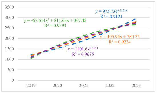
Figure 1.
Fitted Model of SFH’s Operating Revenue.
Table 4.
SFH’s Operating Revenue Forecast for 2024–2028.
The operating costs of SFH primarily include labor costs, transportation capacity costs (such as the purchase, leasing, maintenance of transportation vehicles, and fuel expenses), site and equipment costs, and outsourcing costs for transportation and sorting processes. This paper selects the average proportion of operating costs to operating revenue, which is 85.71%, to predict the future operating costs of SFH. Taxes and surcharges represent a significant expense in business operations, and this paper uses their average proportion of 0.22% of operating revenue for prediction. The average proportions of sales expenses, administrative expenses, and financial expenses are 1.36%, 7.37%, and 0.66%, respectively (see Table 5). Drawing on the prediction methods of the previous two items, these proportions are used as the basis for forecasting future expenses.
Table 5.
SFH’s Related Costs and Expenses from 2019 to 2023.
The forecast results for SFH’s period expenses for 2024–2028 are shown in Table 6.
- 3.
- Capital Expenditures and Increases in Working Capital Forecasts
Table 6.
SFH’s Related Costs and Expenses Forecast for 2024–2028.
The calculation methods for capital expenditures and the increase in working capital are as follows:
Capital expenditures = cash paid by a business to construct fixed assets, intangible assets, and other long-term assets − net cash recovered from the disposal of fixed assets, intangible assets and other long-term assets
Increase in working capital = increase in current assets + increase in current liabilities
SFH’s capital expenditures in 2021 increased by 39.04% year-on-year compared with those in 2020 but decreased by 42.38% year-on-year in 2022 (see Table 7). The significant changes were due to the company’s increased investments in land, warehouses, sorting centers, and vehicles during 2020 and 2021, as well as the impact of the pandemic on the logistics industry, resulting in a larger proportion of capital expenditures. Therefore, to ensure timeliness and rationality, this paper uses the average proportion of capital expenditures (net of disposals) to operating revenue from 2022 to 2023, which is 4.97%, as the basis for forecasting future capital expenditures.
Table 7.
SFH’s Capital Expenditures and Working Capital from 2019 to 2023.
Owing to the susceptibility of working capital to various factors, SFH’s increase in working capital, as a proportion of operating revenue, has fluctuated significantly over the past five years without a clear pattern. This is due to SFH’s increased investments in its four new businesses (pharmaceutical cold chain, international, freight, and intracity) and research, while labor and transportation costs have risen. Therefore, the increase in working capital showed positive growth in 2019, 2021, and 2023 but negative growth in 2020 and 2022. To ensure the accuracy and objectivity of the forecast, the average rate of −1.62% after excluding unstable indicators is used for forecasting. The forecast results for capital expenditures and the increase in working capital for the next five years are shown in Table 8.
- 4.
- Depreciation and Amortization Forecast
Table 8.
SFH’s Capital Expenditures and Increase in Working Capital Forecast for 2024–2028.
SFH’s depreciation and amortization amounts from 2019 to 2023 are shown in Table 9.
Table 9.
SFH’s Depreciation and Amortization Amounts from 2019 to 2023.
To maintain data rationality and validity, the average proportion of depreciation and amortization expenses to operating revenue over the past five years, which is 6.13%, is used as the forecast benchmark. The forecast results for SFH’s depreciation and amortization amounts from 2024 to 2028 are shown in Table 10.
- 5.
- Free Cash Flow Forecast Results
Table 10.
SFH’s Depreciation and Amortization Forecast for 2024–2028.
The forecasted free cash flow for SFH from 2024 to 2028 is summarized in Table 11.
Table 11.
Forecast of Free Cash Flow for SFH (2024–2028).
4.2.2. Forecast of Contribution Values for Various Assets
On the basis of East Money Choice data and the percentage sales method, the average proportions of current assets and fixed assets to operating revenue for SFH over the past five years are calculated to be 37.27% and 17.28%, respectively. The one-year bank loan interest rate of 4.35% is selected as the return rate for current assets, and the five-year bank loan interest rate of 4.65% is selected as the return rate for fixed assets and intangible assets. The contribution values of various assets for the next five years are forecasted accordingly. Table 12 and Table 13 show the forecasted contribution values of current assets and fixed assets for SFH from 2024 to 2028.
Table 12.
Forecast of Contribution Value of Current Assets for SFH (2024–2028).
Table 13.
Forecast of the Contribution Value of Fixed Assets for SFH (2024–2028).
The contribution value of intangible assets consists of on-balance-sheet intangible assets and off-balance-sheet intangible assets. The calculation method is similar to that of fixed assets. This paper uses the five-year bank loan interest rate of 4.65% as the return rate for on-balance-sheet intangible assets. The specific forecast results are shown in Table 14.
Table 14.
Forecast of Contribution Value of On-Balance-Sheet Intangible Assets for SFH. (2024–2028).
4.2.3. Discount Rate Calculation
This study uses the weighted average cost of capital (WACC) as the basis for the discount rate calculation. An analysis of SFH’s financial statements for 2019–2023 reveals that its five-year average gearing ratio is 52.88%, corresponding to a debt capital ratio of 52.88% and an equity capital ratio of 47.12%. The cost of debt capital was 4.9% when the benchmark interest rate for bank loans of five years and above was used, adjusted by the 25% income tax rate of 4.17%. The cost of equity capital is calculated by the capital asset pricing model (CAPM), in which the risk-free interest rate is taken as the five-year treasury bond yield of 3.12%, the market risk premium is calculated on the basis of the arithmetic average return of the CSI 300 index from 2019–2023 of 10.7%, and the β coefficient is 1.35, which results in a final cost of equity of 13.15%. The resulting WACC of SFH is calculated to be 7.95%. To verify the reasonableness of the parameters, this study also calculates the WACC of Yuantong Express (6.68%) and Yunda Express (6.14%) as a comparative reference for the industry, and the specific calculation results are shown in Table 15.
Table 15.
Weighted Average Cost of Capital for Peer Companies.
On the basis of the data in the table above and Formula (4), the return on investment for intangible assets is calculated. The average return on investment for intangible assets across the three companies is 22.58%, as shown in Table 16. This value is used as the discount rate for SFH’s data assets.
Table 16.
Combined Returns on Intangible Assets for SFH.
4.2.4. Calculation of the Data Asset Contribution Rate
This paper draws on the practices of Fu (2024) [] and uses the analytic hierarchy process (AHP) to segment intangible assets. Combining SFH’s business characteristics and profitability, the weight of each individual intangible asset in the excess earnings of off-balance-sheet intangible assets is taken as the goal layer. The results show that the direct reasons for generating excess earnings are product prices being higher than those of similar products from other companies (due to brand premium factors), significant sales growth, increasing competitiveness, and decreasing production and operating costs. Therefore, price advantage, sales growth, competitiveness improvement, and cost savings are selected as the four factors of the criterion layer. Regarding the classification of off-balance sheet intangible assets, drawing on the studies of Li Zhengwei (2019) [] and considering the corporate characteristics of Shunfeng Holdings, off-balance sheet intangible assets are broadly classified into seven categories, namely, goodwill or organizational image, customer relationships, information technology systems, corporate culture, corporate strategic planning and policies, human resources, and data assets. The specific hierarchical structure of the company’s off-balance-sheet intangible asset value is shown in Figure 2.
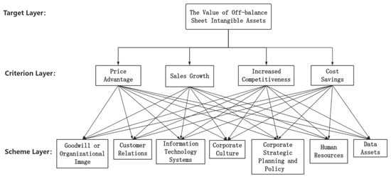
Figure 2.
Hierarchy of the value of off-balance sheet intangible assets of SFH.
On the basis of Figure 2, we invited seven experts, including asset appraisers and managers of SFH, to rate the relative importance of each factor at the guideline level quantitatively by using the sum-and-product method and pairwise comparisons of the evaluation indicators on a scale of 1–9 through a questionnaire star, and the results are shown in Table 17.
Table 17.
Assignment Results of the Criterion Layer Judgment Matrix.
By normalizing the judgment matrix, the eigenvectors and weights of the four indicators in the criterion layer—price advantage, sales growth, competitiveness improvement, and cost savings—are obtained, as shown in Table 18.
Table 18.
Weights of Criterion Layer Indicators.
To avoid the influence of subjective factors in expert judgments, a consistency check is performed on the criterion layer’s judgment matrix. On the basis of the judgment matrix results, the maximum eigenvalue is calculated as 16.0622, and the maximum eigenvalue is 4.0156. The numerical results of each indicator are shown in Table 19.
Table 19.
Consistency Check Results of the Criterion Layer Judgment Matrix.
On the basis of the secondary indicators in the hierarchical structure diagram, the weights of the indicators in the solution layer are calculated by establishing a judgment matrix. The specific results are shown in Table 20.
Table 20.
Weights of the indicators in the solution layer.
On the basis of the analysis results of each factor indicator, the data asset contribution rate is calculated as 0.2861 (28.61%).
4.2.5. Data Asset Value Assessment Results and Discussion
- Results
The value of SFH’s data assets is then calculated according to the data asset contribution rate, and the results are shown in Table 21.
- 2.
- Discussion
Table 21.
Valuation Results of SFH’s Data Assets (Unit: RMB 100 million).
From the valuation results in Table 21, the present values of SFH’s data assets from 2024 to 2028 are RMB 406.10 million, RMB 381.72 million, RMB 399.21 million, RMB 416.45 million, and RMB 433.38 million, respectively, with a total present value of RMB 2.03686 billion over five years. Although the value of data assets is increasing annually, its proportion of the overall corporate value remains low, indicating that the potential of data assets has not been fully realized.
- (1)
- Dynamics of Data Asset Value and Industry Characterization: Table 21 shows that the present value of data assets for SFH is RMB 2036.87 million from 2024 to 2028, which accounts for only 1.8% of its enterprise free cash flow (RMB 112.86 billion) in the same period. Despite the year-on-year increase in the value of data assets, their share of the overall value of the enterprise remains low. On the one hand, this reflects the asset-heavy nature of the logistics industry, with the total value of fixed assets contributed by SFH over the five-year period amounting to RMB 56.992 billion, accounting for 50.5% of the enterprise’s free cash flow over the same period (based on the summary calculation in Table 13 and Table 11), and the release of the value of data assets being constrained by the synergistic efficiency of the physical network (e.g., picking centers, transportation means). On the other hand, it also shows that the potential of data assets has not been fully released. As a leading logistics company, SFH owns a large amount of data, but there is still more room for the deep excavation and value release of data assets.
- (2)
- Validation and analysis of the split rate (K = 28.61%): The result of the split rate derived from this study passed a rigorous validation procedure: a side-by-side comparison revealed that the value was higher than the AHP measurements of Jingdong Logistics [] but lower than the median split rate of the maritime data asset trading market []. This difference may stem from two factors: on the one hand, SFH’s customer relationship data (weight 17.49%) exhibit relatively low value density due to its high proportion of B-side business; on the other hand, the scarcity characteristic of its cold chain data offsets the timeliness disadvantage to some extent. In terms of longitudinal validation, compared with the actual share rate of SFH’s 2024 data asset securitization project (26.9%), the error of the model results is only 6.3%, which fully proves the accuracy of the AHP weight assignment and provides strong support for the practical value of the model.
4.2.6. Sensitivity Analysis
To verify the robustness of the valuation results, this paper performs a two-factor sensitivity analysis (see Figure 3) on the discount rate (±2.5%) and the earnings period (4–6 years). The results show that data asset valuations are more sensitive to changes in the discount rate, with a 1% change in the discount rate affecting valuations 2.3 times more strongly than a change in the earnings period. The optimal scenario with a discount rate of 15.08% and an income period of 6 years results in a valuation of up to CNY 469 million, whereas the worst scenario with a discount rate of 30.08% and an income period of 4 years results in a valuation of only CNY 392 million. The valuation under the baseline scenario (discount rate of 22.58% and an income period of 5 years) is CNY 433 million. The analysis reveals an accelerating downward trend in valuation when the discount rate exceeds 25.08% or the earning period is shorter than 5 years. Notably, the discount rate of 20.08% is a key threshold below which valuations are more sensitive to changes in the earnings period. These findings provide important insights for enterprises’ data asset management: first, the discount rate should be controlled within 25% by improving data quality and expanding realization channels, and second, a 5-year earning period can better balance value capture and prediction risk and is the optimal selection period.
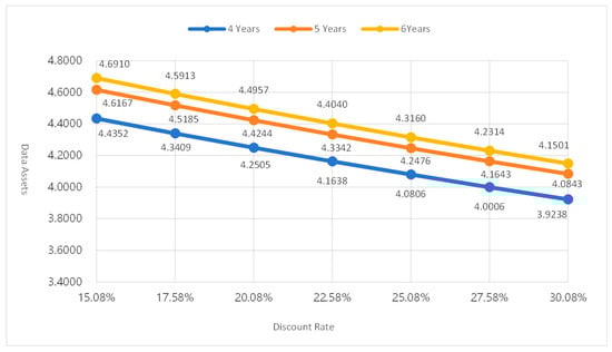
Figure 3.
Sensitivity test plot of the data asset valuation to discount rate vs. period of return.
Notably, there are several limitations in this analysis, including the assumption of a linear relationship between the cash flow and the revenue period, the failure to consider the impact of technology iteration, and the fixed value of the contribution rate K (28.61%). Nonetheless, the analysis results still show that the valuation fluctuation can be controlled within ±15% under conventional conditions (discount rate of 20–25% and earnings period of 5 years), which proves that the valuation model has good robustness.
5. Conclusions
This study provides a new methodological framework for assessing the data asset value of logistics enterprises by constructing a hybrid MPEEM–AHP valuation model. The study confirms that the model is able to address the deficiencies of traditional valuation methods effectively in time-sensitive data value capture and precise segmentation of intangible assets through the dynamic weight adjustment mechanism and hierarchical revenue segmentation algorithm. The case study shows that the model has good applicability in the empirical application of Shunfeng Holdings, and its valuation results are highly consistent with the market data of the enterprise’s actual data asset securitization project.
However, several important limitations remain in this study. First, the subjectivity of expert judgment in the AHP method is still a potential source of error, although it is calibrated by market data. Second, the model does not take into account the sudden changes in data value that may be caused by technological changes, especially the substitution effect of AI technology on traditional logistics data. Finally, the current model is applicable mainly to heavy-asset-based logistics enterprises, and its applicability to light asset models is not fully verified.
On the basis of the research findings, we suggest that logistics enterprises focus on the following aspects of data asset management: establishing a differentiated data asset classification system to distinguish between highly time-sensitive data and long-term value data; prioritizing the development of vertical data products with scarcity; and strengthening the risk assessment and disclosure mechanism of data assets. These suggestions are directly derived from the logistics data value formation law found in the model’s application.
Future research could explore the following directions in depth: developing more objective weight determination algorithms to reduce subjective bias, establishing dynamic industry benchmark data to enhance forecast reliability, and expanding the model’s application in cross-border data asset valuation. These improvements will further increase the accuracy and applicability of the valuation model.
Author Contributions
Conceptualization, L.Y. and S.Q.; Methodology, S.Q.; Software, S.Q. and N.Z.; Validation, L.Y., S.Q. and Z.Y.; Formal analysis, L.Y. and S.Q.; Investigation, S.Q.; Resources, N.Z. and Z.Y.; Data curation, S.Q.; Writing—original draft preparation, L.Y. and S.Q.; Writing—review and editing, L.Y. and Z.Y.; Visualization, S.Q.; Supervision, Z.Y.; Project administration, N.Z.; Funding acquisition, L.Y. All authors have read and agreed to the published version of the manuscript.
Funding
This research was funded by the 2021 Key Projects for General of Universities of Guangdong Province, grant number 2021ZDZX3028.
Institutional Review Board Statement
Ethical review and approval were waived for this study in accordance with the local legislation and institutional requirements (Article 32 of Measures for Ethical Review of Life Sciences and Medical Research Involving Human Beings of China; detailed information can be found at (https://www.gov.cn/zhengce/zhengceku/2023-02/28/content_5743658.htm, accessed on 20 September 2023), as it did not entail clinical trials or manipulations involving humans or animals.
Informed Consent Statement
Informed consent was obtained from all subjects involved in the study.
Data Availability Statement
The data presented in this study are available on request from the corresponding author due to containing business sensitive information protected under non-disclosure agreements.
Conflicts of Interest
The authors declare no conflicts of interest.
References
- Rachana Harish, A.; Liu, X.L.; Zhong, R.Y.; Huang, G.Q. Log-flock: A blockchain-enabled platform for digital asset valuation and risk assessment in E-commerce logistics financing. Comput. Ind. Eng. 2021, 151, 107001. [Google Scholar] [CrossRef]
- Awain, A.M.S.B.; Asad, M.; Sulaiman, M.A.B.A.; Asif, M.U.; Shanfari, K.S. Impact of supply chain risk management on product innovation performance of Omani SMEs: Synergetic moderation of technological turbulence and entrepreneurial networking. Sustainability 2025, 17, 2903. [Google Scholar] [CrossRef]
- Elvina, P.S. The effect of company size, profitability, economic growth rate, market traction and competitive advantage on startup valuation in logistics aggregators. Am. J. Econ. Manag. Bus. 2023, 2, 164–174. [Google Scholar] [CrossRef]
- Lim, S.; Lee, C.-H.; Bae, J.-H.; Jeon, Y.-H. Identifying the optimal valuation model for maritime data assets with the Analytic Hierarchy Process (AHP). Sustainability 2024, 16, 3284. [Google Scholar] [CrossRef]
- Yuswadi, M.R.A.-N.; Soekarno, S. Digital transformation and corporate valuation: Unveiling the influence of digital maturity in stocks return in Indonesian FMCG industry. Int. J. Curr. Sci. Res. Rev. 2024, 7, 4553–4558. [Google Scholar] [CrossRef]
- Bang, S.-H.; Lee, K.-H.; Jang, J.-Y.; Seon, H.-N.; Shin, K.-S. Prioritization on information sharing in digital platform for linking online retail and logistics systems using AHP. Korean Logist. Res. Assoc. 2023, 33, 45–57. [Google Scholar] [CrossRef]
- Tang, Z. Research on the accounting recognition and measurement problems of enterprise data assets. Int. J. Glob. Econ. Manag. 2024, 3, 242–253. [Google Scholar] [CrossRef]
- Fu, J.; Xiao, B.; Wang, F. Evaluation of data asset value based on Hierarchical Analysis Method. Front. Bus. Econ. Manag. 2024, 12, 240–244. [Google Scholar] [CrossRef]
- Yin, C.; Jin, T.; Zhang, P.; Wang, J.; Chen, J. Assessment and pricing of data assets: Research review and prospect. Big Data Res. 2021, 7, 14–27. [Google Scholar]
- Simanjuntak, D.; Nurjanah, S.; Willy; Muda, I. Historical cost vs current cost accounting method. Braz. J. Dev. 2023, 9, 31828–31840. [Google Scholar] [CrossRef]
- Gad, I. Challenges in asset and liability valuation: Bridging fair value and historical cost accounting. South Asian J. Soc. Stud. Econ. 2024, 21, 10–17. [Google Scholar] [CrossRef]
- Nada, E.Q.; Novitasari, S.B.; Putri, Q.L.; Wahyuni, N. Market value analysis of Dalwa Syariah Hotel with cost approach and income approach methods. J. Akunt. Terap. Dan Bisnis 2022, 2, 1–11. [Google Scholar] [CrossRef]
- Martin, D.; Heinz, D.; Glauner, M.; Kuhl, N. Selecting data assets in data marketplaces: Leveraging machine learning and explainable AI for value quantification. Bus. Inf. Syst. Eng. 2025. [Google Scholar] [CrossRef]
- Zhang, J.; Dong, W.; Wei, Y. Business big data analysis: Research on valuation methods of transactional data assets. J. Intell. 2023, 7, 1–33. (In Chinese) [Google Scholar]
- Li, W.; Yang, W.; Zhou, Z.; Wu, S.; Mo, C. Analyzing the game pricing mechanism of data assets: Theoretical evidence considering market structure and competitive characteristics. Int. Rev. Econ. Financ. 2025, 99, 104043. [Google Scholar] [CrossRef]
- Lev, B.; Feng, G. The End of Accounting and the Path Forward for Investors and Managers; John Wiley & Sons: Hoboken, NJ, USA, 2016. [Google Scholar]
- Zhou, X.; Zhang, B. Valuation of enterprise data assets by using the improved multi-period excess-earnings method. J. Ind. Eng. Manag. 2023, 1, 24–31. [Google Scholar] [CrossRef]
- Feng, L.; Hu, X.; Zhao, X. Research on data asset valuation based on lifecycle theory: A case study of Bilibili. Friends Account. 2024, 13, 15–21. (In Chinese) [Google Scholar]
- Saaty, T.L. A scaling method for priorities in hierarchical structures. J. Math. Psychol. 1977, 15, 234–281. [Google Scholar] [CrossRef]
- Kaewfak, K.; Huynh, V.-N.; Ammarapala, V.; Charoensiriwath, C. A fuzzy AHP-TOPSIS approach for selecting the multimodal freight transportation routes. In Communications in Computer and Information Science; Springer: Singapore, 2019; pp. 28–46. [Google Scholar]
- Rashidi, K. AHP versus DEA: A comparative analysis for the gradual improvement of unsustainable suppliers. Benchmarking Int. J. 2020, 27, 2283–2321. [Google Scholar] [CrossRef]
- Cao, X. E-commerce platform risk identification using AHP hierarchical analysis and BPNN neural network. In Proceedings of the 2022 2nd International Signal Processing, Communications and Engineering Management Conference (ISPCEM), Montreal, ON, Canada, 25–27 November 2022; pp. 316–323. [Google Scholar]
- Yang, H.; Zhang, Y.; Ma, H. Evaluation model and promotion of logistics transportation D and A system based on AHP. In Proceedings of the 3rd International Conference on Applied Mathematics, Modelling, and Intelligent Computing, Tangshan, China, 24–26 March 2023; p. 175. [Google Scholar]
- Surucu-Balci, E.; Iris, Ç.; Balci, G. Digital information in maritime supply chains with blockchain and cloud platforms: Supply chain capabilities, barriers, and research opportunities. Technol. Forecast. Soc. Change 2024, 198, 122978. [Google Scholar] [CrossRef]
- Wang, J.; Li, H.; Guo, H. Coordinated development of logistics development and low-carbon environmental economy base on AHP-DEA model. Sci. Program. 2022, 1, 5891909. [Google Scholar] [CrossRef]
- Yang, Y.; Guo, Z.; Zhang, L.; Sun, L. Analysis of the implementation path of data asset valorization. Inf. Commun. Technol. Policy 2024, 50, 24–33. (In Chinese) [Google Scholar]
- Li, Z. Research on the valuation system of off-balance-sheet intangible assets. Commer. Account. 2019, 13, 90–92. (In Chinese) [Google Scholar]
Disclaimer/Publisher’s Note: The statements, opinions and data contained in all publications are solely those of the individual author(s) and contributor(s) and not of MDPI and/or the editor(s). MDPI and/or the editor(s) disclaim responsibility for any injury to people or property resulting from any ideas, methods, instructions or products referred to in the content. |
© 2025 by the authors. Licensee MDPI, Basel, Switzerland. This article is an open access article distributed under the terms and conditions of the Creative Commons Attribution (CC BY) license (https://creativecommons.org/licenses/by/4.0/).