Analysing the Influence of Macroeconomic Factors on Credit Risk in the UK Banking Sector


Abstract
1. Introduction
- How did the UK’s macroeconomic factors and credit risk change over the time from 2005 to 2021?
- What was the effect of macroeconomic factors on credit risk from 2005 to 2021?
- How are macroeconomic factors and banking credit risk related?
- Which machine learning (ML) model can outperform conventional regression models for credit risk prediction?
2. Related Work
2.1. Theme 1: Credit Risk Definition, Indicators, and Implications
2.2. Theme 2: Selection of Credit Risk (NPL) Determinant Types
2.3. Theme 3: Macroeconomic Determinants of Credit Risk
2.4. Theme 4: Credit Risk Predictive Models Using Macroeconomic Determinants
2.5. Theme 5: Data Visualization of Credit Risk and Its Macroeconomic Determinants
3. Methodology
3.1. Variable Selection Technique
3.2. Data Processing
3.2.1. Removal of Duplicate Records
3.2.2. Handling of Missing Data
3.2.3. Variable Renaming, Uniform Formatting, and Sorting
3.2.4. Dealing with Outliers
3.3. Data Transformation
3.3.1. Append Data
3.3.2. Create New Binary Target Variable
4. Results
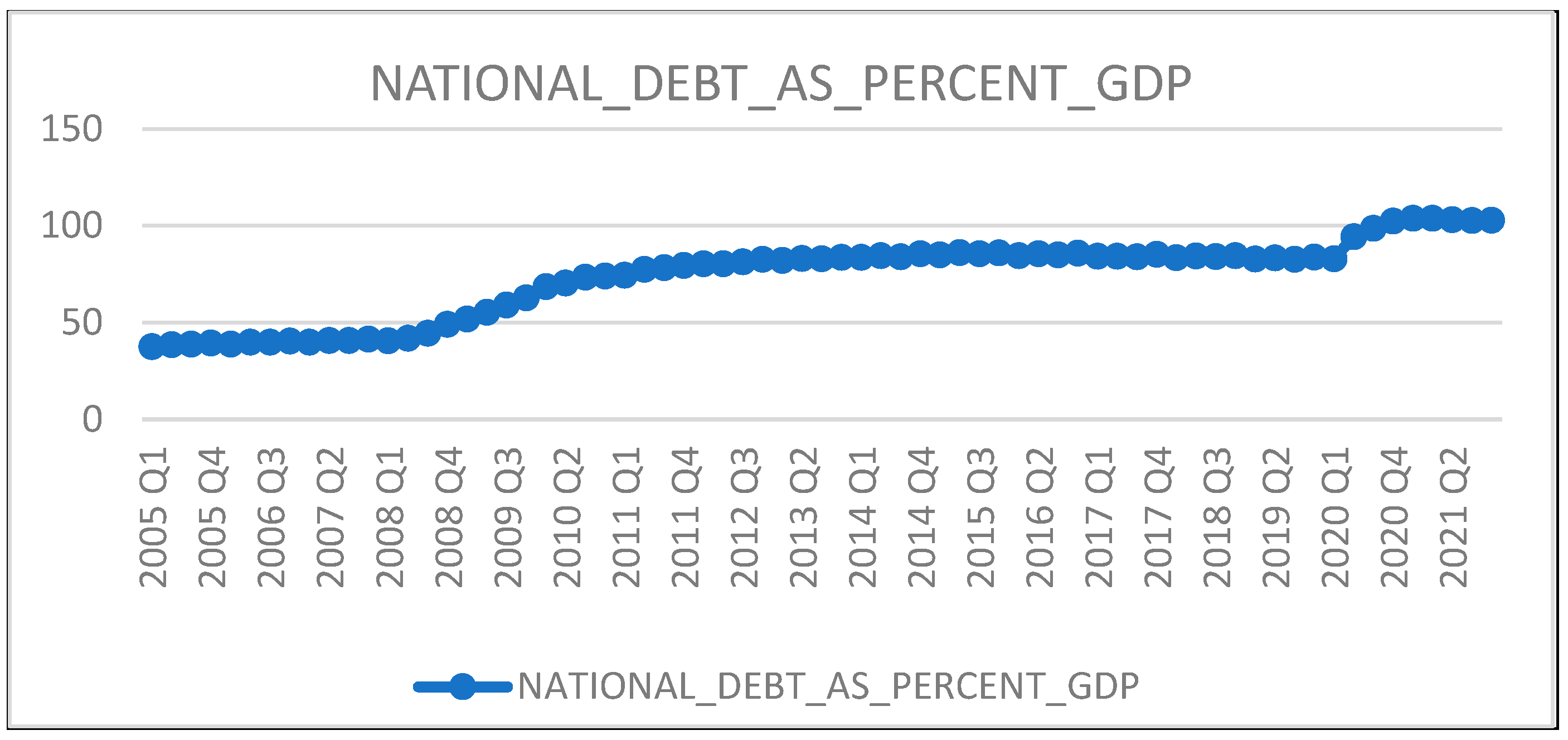
4.1. Trend Analysis
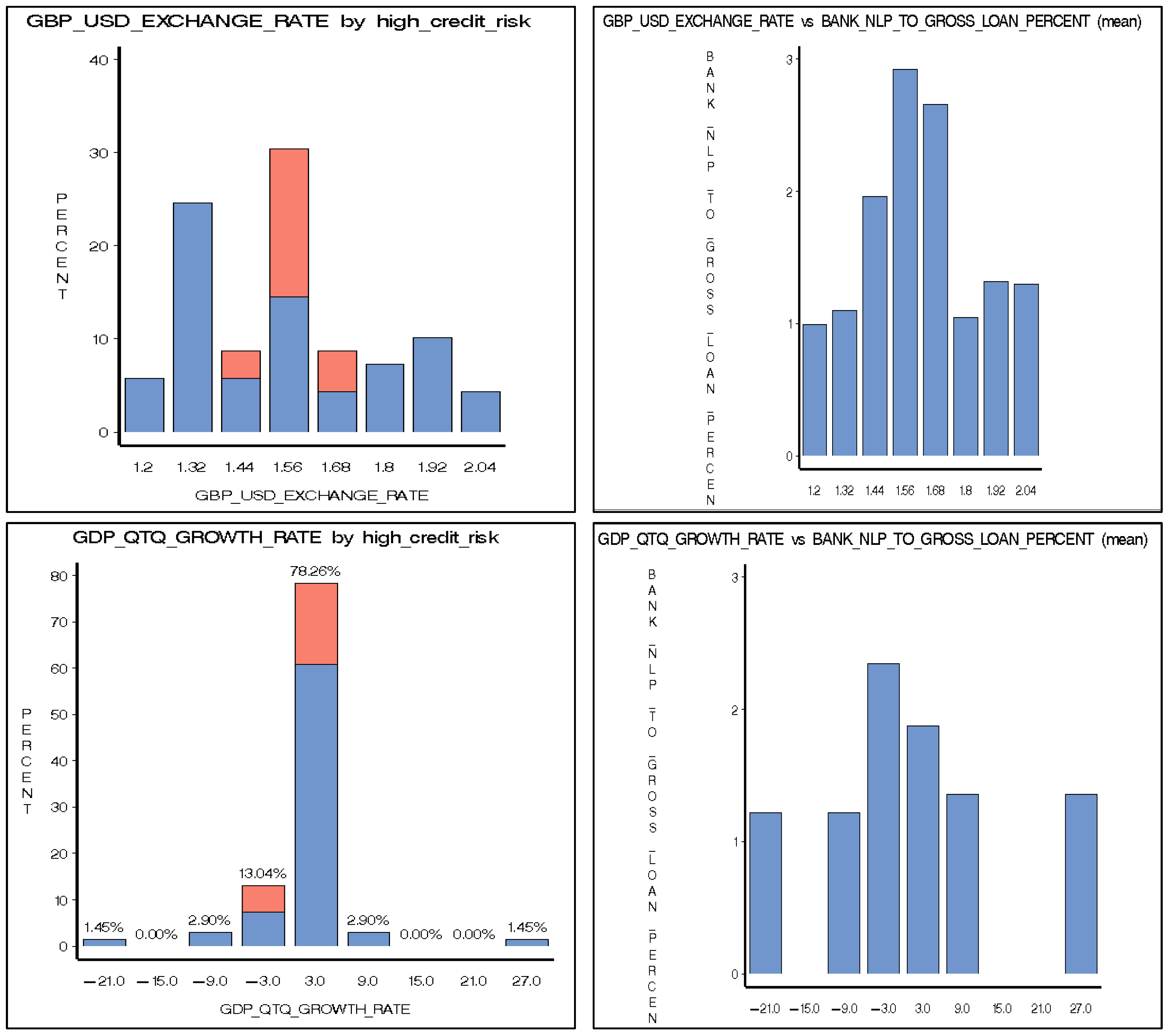
4.2. Multidimensional Analysis
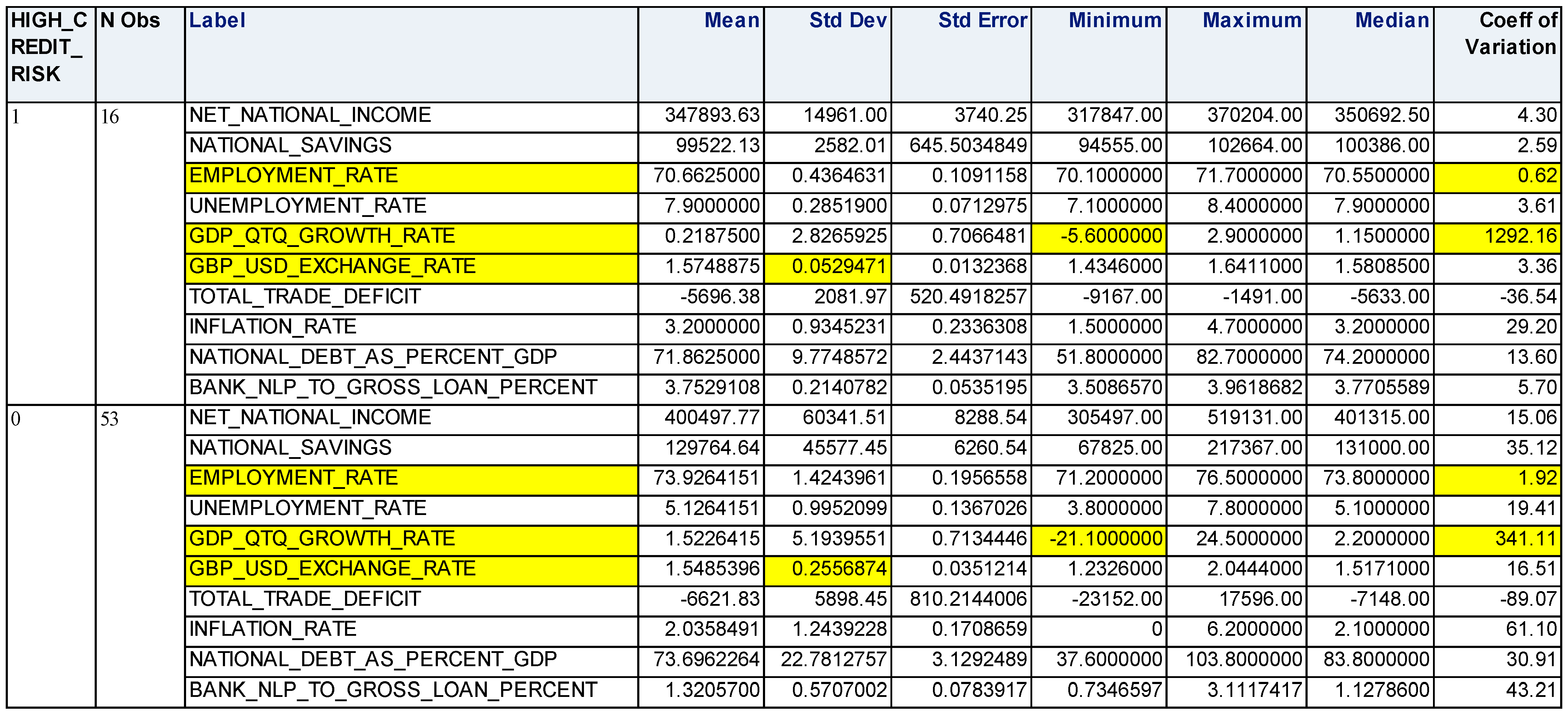
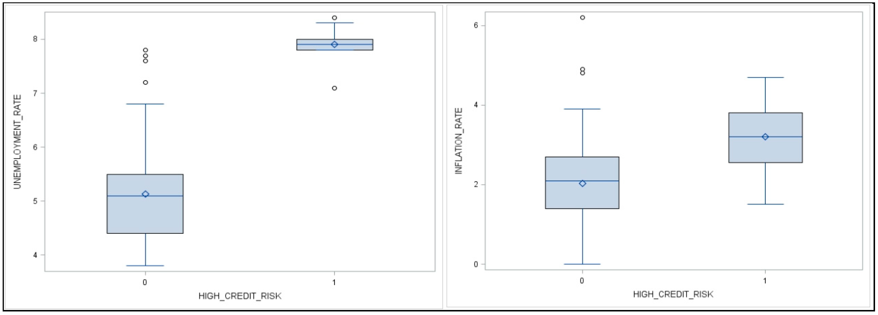
4.3. Descriptive Analysis
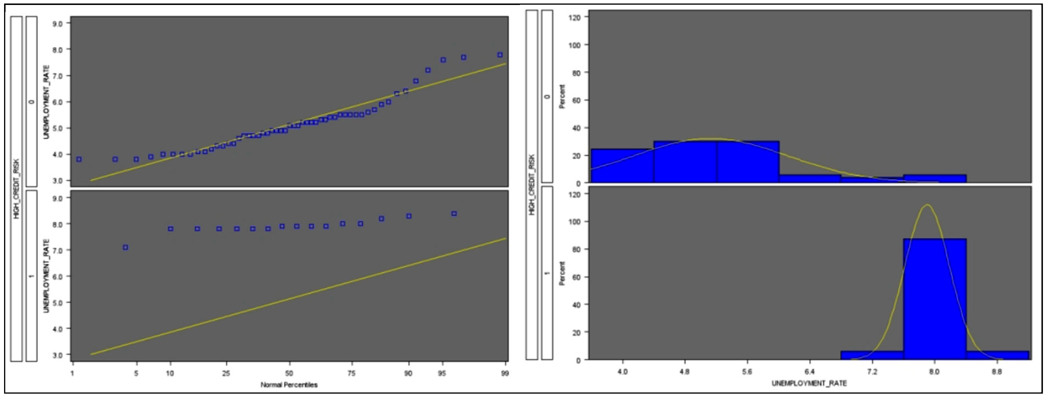
4.4. Distribution Analysis
4.5. Multicollinearity
4.6. Diagnostic Analysis
4.7. Discussion
4.7.1. Logistic Regression
4.7.2. Neural Network
4.7.3. Decision Tree
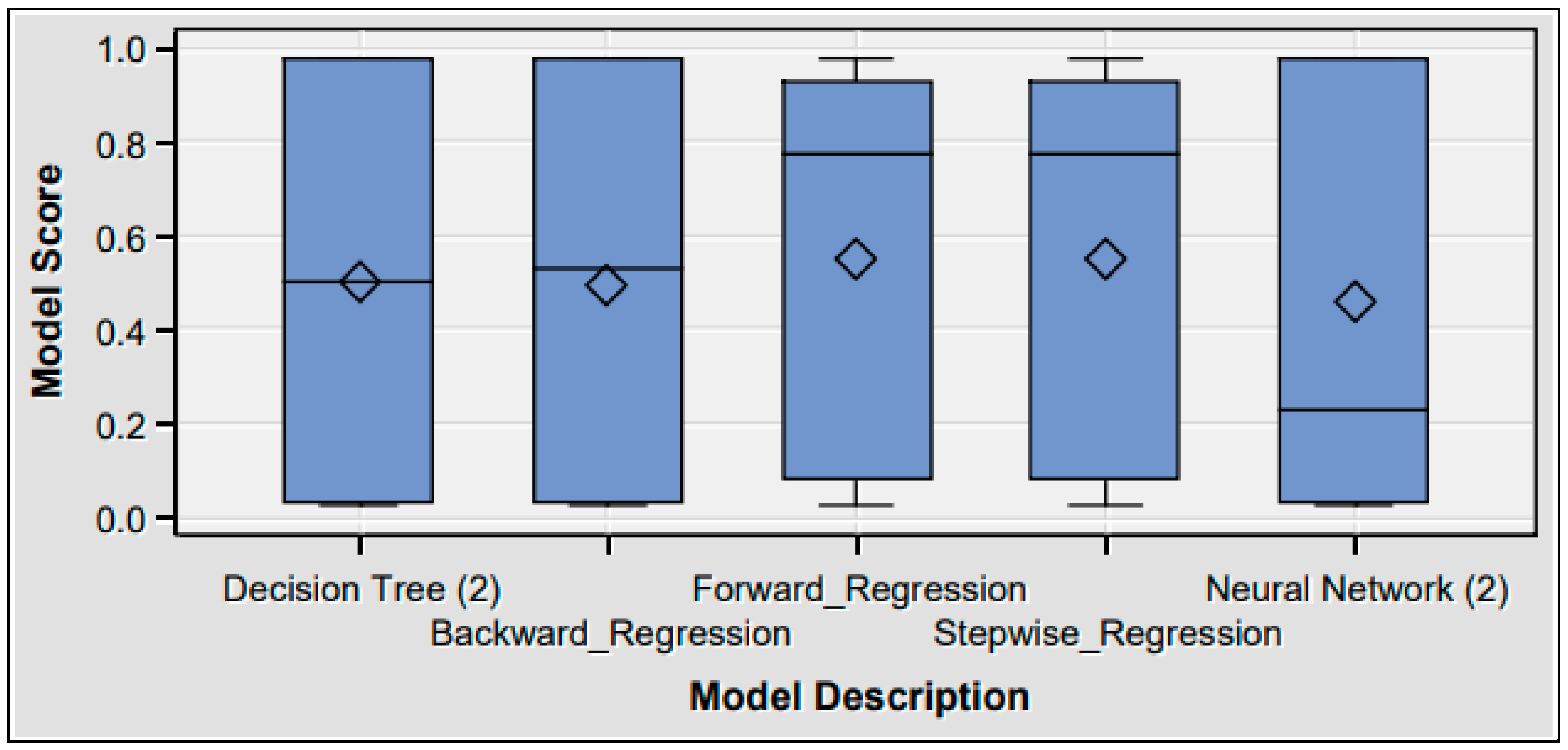
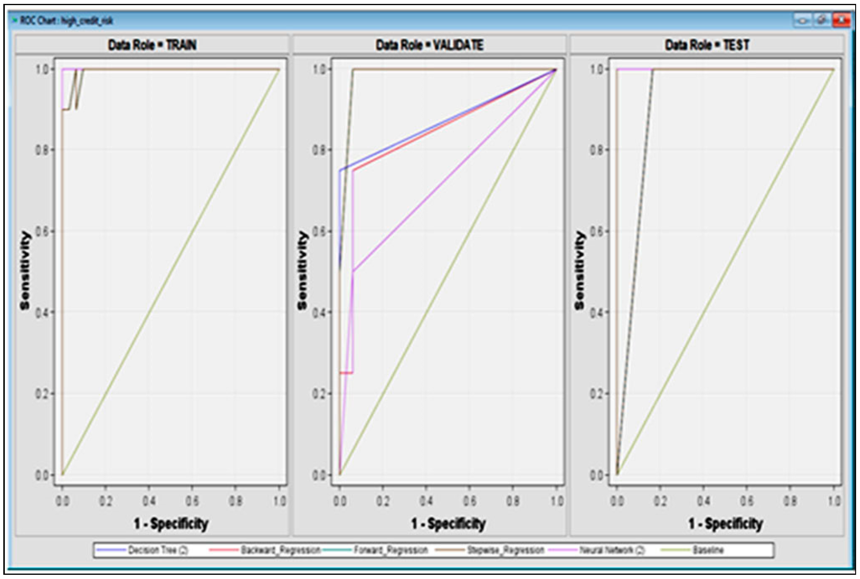
4.7.4. Predictive Models’ Comparison
5. Conclusions
- To assure unaffected, reliable, accurate outcomes, we recommend conducting multicollinearity and trend analysis prior to commencing predictive data modelling;
- To improve predictive modelling execution, it is advisable to use missing data imputation, making aesthetic adjustments such as renaming, using consistent formatting for all variables in ascending order;
- This research employs yet another best practise, the extensive analysis of outliers, by analysing measures like leverage, deleted residuals, and the covariance ratio;
- For highly structured, normally distributed, quantitative data, the stratified technique of data partitioning is recommended, as it produces precise testing results with minimum variation compared to the simple random method with a comparable sample size.
Author Contributions
Funding
Institutional Review Board Statement
Informed Consent Statement
Data Availability Statement
Conflicts of Interest
List of Abbreviations
| Analytics Software & Solutions | SAS |
| United Kingdom | UK |
| Bank of England | BOE |
| International Monetary Fund | IMF |
| Association for Computing Machinery | ACM |
| European Union | EU |
| Cross-industry standard Data Mining | CRISP-DM |
| General Data Protection Regulation | GDPR |
| UK Office for National Statistics | ONS |
| Decision support system | DSS |
| Machine learning | ML |
| Information value | IV |
| Non-performing assets | NPA |
| Ratio of capital adequacy | CAR |
| Non-performing loan | NPL |
| Gross Domestic Product | GDP |
| Great British Pound | GBP |
| United States Dollar | USD |
| Receiver Operating Characteristic Curve | ROC |
| Variance Inflation Factor | VIF |
| Complex event processing | CEP |
| Quantile–Quantile |
References
- Fainstein, G.; Novikov, I. The comparative analysis of credit risk determinants in the banking sector of the Baltic States. Rev. Econ. Financ. 2011, 1, 20–45. [Google Scholar]
- Reinhart, C.M.; Rogoff, K.S. From Financial Crash to Debt Crisis. Am. Econ. Rev. 2011, 101, 1676–1706. [Google Scholar] [CrossRef]
- IMF Country Report. United Kingdom: Financial Sector Assessment Program-Systemic Stress, and Climate-Related Financial Risks: Implications for Balance Sheet Resilience (imf.org). 8 April 2022. Available online: https://www.imf.org/en/Publications/CR/Issues/2022/04/07/United-Kingdom-Financial-Sector-Assessment-Program-Systemic-Stress-and-Climate-Related-516264 (accessed on 1 May 2022).
- Carvalho, P.V.; Curto, J.D.; Primor, R. Macroeconomic determinants of credit risk: Evidence from the Eurozone. Int. J. Financ. Econ. 2022, 27, 2054–2072. [Google Scholar] [CrossRef]
- Monetary Policy Report. Bank of England Monetary Policy Report August 2022. August 2022. Available online: https://www.bankofengland.co.uk/-/media/boe/files/monetary-policy-report/2022/august/monetary-policy-report-august-2022.pdf (accessed on 1 May 2022).
- Yu, J. Big Data Analytics and Discrete Choice Model for Enterprise Credit Risk Early Warning Algorithm. Secur. Commun. Netw. 2022, 2022, 3272603. [Google Scholar] [CrossRef]
- Ghosh, A. Managing Risks in Commercial and Retail Banking. In Managing Risks in Commercial and Retail Banking; John Wiley & Sons: Singapore, 2012. [Google Scholar] [CrossRef]
- Pagdin, I.; Hardy, M. Investment and Portfolio Management: A Practical Introduction; KoganPage: London, UK, 2018. [Google Scholar]
- Khandani, A.E.; Kim, A.J.; Lo, A.W. Consumer credit-risk models via machine-learning algorithms. J. Bank. Financ. 2010, 34, 2767–2787. [Google Scholar] [CrossRef]
- Ghosh, A. Banking-industry specific and regional economic determinants of non-performing loans: Evidence from US states. J. Financ. Stab. 2015, 20, 93–104. [Google Scholar] [CrossRef]
- Makri, V.; Tsagkanos, A.; Bellas, A. Determinants of non-performing loans: The case of Eurozone. Panoeconomicus 2014, 61, 193–206. [Google Scholar] [CrossRef]
- Hersugondo, H.; Anjani, N.; Pamungkas, I.D. The Role of Non-Performing Asset, Capital, Adequacy and Insolvency Risk on Bank Performance: A Case Study in Indonesia. J. Asian Financ. Econ. Bus. 2021, 8, 319–329. [Google Scholar]
- Louzis, D.P.; Vouldis, A.T.; Metaxas, V.L. Macroeconomic and bank-specific determinants of non-performing loans in Greece: A comparative study of mortgage, business and consumer loan portfolios. J. Bank. Financ. 2012, 36, 1012–1027. [Google Scholar] [CrossRef]
- Bolisani, E.S.E. How corruption affects loan portfolio quality in emerging markets? J. Financ. Crime 2016, 23, 769–785. [Google Scholar] [CrossRef]
- Salas, V.; Saurina, J. Credit risk in two institutional regimes: Spanish commercial and savings banks. J. Financ. Serv. Res. 2002, 22, 203–224. [Google Scholar] [CrossRef]
- Amuakwa-Mensah, F.; Marbuah, G.; Ani-Asamoah Marbuah, D. Re-examining the determinants of non-performing loans in Ghana’s banking industry: Role of the 2007–2009 financial crisis. J. Afr. Bus. 2017, 18, 357–379. [Google Scholar] [CrossRef]
- Ghosh, A. Sector-specific analysis of non-performing loans in the US banking system and their macroeconomic impact. J. Econ. Bus. 2017, 93, 29–45. [Google Scholar] [CrossRef]
- Kjosevski, J.; Petkovski, M.; Naumovska, E. Bank-specific and macroeconomic determinants of non-performing loans in the Republic of Macedonia: Comparative analysis of enterprise and household NPLs. Econ. Res. Ekon. Istraživanja 2019, 32, 1185–1203. [Google Scholar] [CrossRef]
- Konstantakis, K.N.; Michaelides, P.G.; Vouldis, A.T. Non-performing loans (NPLs) in a crisis economy: Long-run equilibrium analysis with a real time VEC model for Greece (2001–2015). Phys. A 2016, 451, 149–161. [Google Scholar] [CrossRef]
- Corden, W.M. Global imbalances and the paradox of thrift. Oxf. Rev. Econ. Policy 2012, 28, 431–443. [Google Scholar] [CrossRef]
- Thurik, A.R.; Carree, M.A.; van Stel, A.; Audretsch, D.B. Does self-employment reduce unemployment? J. Bus. Ventur. 2008, 23, 673–686. [Google Scholar] [CrossRef]
- Lindbeck, A.; Snower, D.J. EXPLANATIONS OF UNEMPLOYMENT. Oxf. Rev. Econ. Policy 1985, 1, 34–59. [Google Scholar] [CrossRef]
- Kuzucu, N.; Kuzucu, S. What drives non-performing loans? Evidence from emerging and advanced economies during pre- and post-global financial crisis. Emerg. Mark. Financ. Trade 2019, 55, 1694–1708. [Google Scholar] [CrossRef]
- Klein, N. Non-Performing Loans in CESEE: Determinants and Impact on Macroeconomic Performance. In Policy File; International Monetary Fund: Washington, DC, USA, 2013. [Google Scholar]
- Gulati, R.; Goswami, A.; Kumar, S. What drives credit risk in the Indian banking industry? An empirical investigation. Econ. Syst. 2019, 43, 42–62. [Google Scholar] [CrossRef]
- Nkusu, M. Nonperforming loans and macro financial vulnerabilities in advanced economies. IMF Work. Pap. 2011, 11, 1. [Google Scholar] [CrossRef]
- Umar, M.; Sun, G. Determinants of non-performing loans in Chinese banks. J. Asia Bus. Stud. 2018, 12, 273–289. [Google Scholar] [CrossRef]
- Beck, R.; Jakubik, P.; Piloiu, A. Key determinants of non-performing loans: New evidence from a global sample. Open Econ. Rev. 2015, 26, 525–550. [Google Scholar] [CrossRef]
- Gila-Gourgoura, E.; Nikolaidou, E. Credit Risk Determinants in the Vulnerable Economies of Europe: Evidence from the Spanish Banking System. Int. J. Bus. Econ. Sci. Appl. Res. 2017, 10, 60–71. [Google Scholar] [CrossRef]
- Krumeich, J.; Werth, D.; Loos, P. Prescriptive Control of Business Processes: New Potentials Through Predictive Analytics of Big Data in the Process Manufacturing Industry. Bus. Inf. Syst. Eng. 2015, 58, 261–280. [Google Scholar] [CrossRef]
- Dixon, M.F.; Halperin, I.; Bilokon, P. Machine Learning in Finance; Springer International Publishing: New York, NY, USA, 2020; Volume 1406. [Google Scholar] [CrossRef]
- Ouahilal, M.; El Mohajir, M.; Chahhou, M.; El Mohajir, B.E. A comparative study of predictive algorithms for business analytics and decision support systems: Finance as a case study. 2016 International Conference on Information Technology for Organizations Development (IT4OD), Fez, Morocco, 30 March–1 April 2016; pp. 1–6. [Google Scholar] [CrossRef]
- Wang, T.; Zhao, S.; Zhu, G.; Zheng, H. A machine learning-based early warning system for systemic banking crises. Appl. Econ. 2021, 53, 2974–2992. [Google Scholar] [CrossRef]
- Fitzpatrick, T.; Mues, C. An empirical comparison of classification algorithms for mortgage default prediction: Evidence from a distressed mortgage market. Eur. J. Oper. Res. 2016, 249, 427–439. [Google Scholar] [CrossRef]
- Hosmer, D.W., Jr.; Lemeshow, S.; Sturdivant, R.X. Applied Logistic Regression, 3rd. ed.; Wiley: Hoboken, NJ, USA, 2013. [Google Scholar]
- Broby, D. The use of predictive analytics in finance. J. Financ. Data Sci. 2022, 8, 145–161. [Google Scholar] [CrossRef]
- Hu, X.-Y.; Tang, Y. Ann-based credit risk identification and control for commercial banks. In Proceedings of the 2006 International Conference on Machine Learning and Cybernetics, Dalian, China, 13–16 August 2006; pp. 3110–3114. [Google Scholar] [CrossRef]
- Baesens, B.; Setiono, R.; Mues, C.; Vanthienen, J. Using Neural Network Rule Extraction and Decision Tables for Credit-Risk Evaluation. Manag. Sci. 2003, 49, 312–329. [Google Scholar] [CrossRef]
- Ruiz, S.; Gomes, P.; Rodrigues, L.; Gama, J. Credit Scoring in Microfinance Using Non-traditional Data. In Progress in Artificial Intelligence. EPIA 2017; Oliveira, E., Gama, J., Vale, Z., Lopes Cardoso, H., Eds.; Lecture Notes in Computer Science; Springer: Cham, Switzerland, 2017; Volume 10423. [Google Scholar] [CrossRef]
- Kotsiantis, S.; Koumanakos, E.; Tzelepis, D.; Tampakas, V. Predicting Fraudulent Financial Statements with Machine Learning Techniques. In Advances in Artificial Intelligence. SETN 2006; Antoniou, G., Potamias, G., Spyropoulos, C., Plexousakis, D., Eds.; Lecture Notes in Computer Science; Springer: Berlin/Heidelberg, Germany, 2006; Volume 3955. [Google Scholar] [CrossRef]
- Lang, J.; Sun, J. Sensitivity of decision tree algorithm to class-imbalanced bank credit risk early warning. In Proceedings of the 2014 Seventh International Joint Conference on Computational Sciences and Optimization, Beijing, China, 4–6 July 2014; pp. 539–543. [Google Scholar] [CrossRef]
- Clements, J.M.; Xu, D.; Yousefi, N.; Efimov, D. Sequential Deep Learning for Credit Risk Monitoring with Tabular Financial Data. arXiv 2020, arXiv:2012.15330. [Google Scholar]
- Calibo, D.I.; Ballera, M.A. Variable selection for credit risk scoring on loan performance using regression analysis. In Proceedings of the 2019 IEEE 4th International Conference on Computer and Communication Systems (ICCCS), Singapore, 23–25 February 2019; pp. 746–750. [Google Scholar] [CrossRef]
- Chu, M.K.; Yong, K.O. Big Data Analytics for Business Intelligence in Accounting and Audit. Open J. Soc. Sci. 2021, 9, 42–52. [Google Scholar] [CrossRef]
- ACM Council. Code of Ethics—ACM Ethics. 22 June 2018. Available online: https://ethics.acm.org/code-of-ethics/ (accessed on 1 May 2022).
- Worldbank Datasource. Bank Nonperforming Loans to Total Gross Loans (%)—United Kingdom|Data (worldbank.org). Available online: https://data.worldbank.org/indicator/FB.AST.NPER.ZS?locations=GB (accessed on 1 May 2022).
- UK ONS Datasource. Home—Office for National Statistics (ons.gov.uk). Available online: https://www.ons.gov.uk (accessed on 1 May 2022).
- Foster, D.P.; Stine, R.A. Variable Selection in Data Mining: Building a Predictive Model for Bankruptcy. J. Am. Stat. Assoc. 2004, 99, 303–313. [Google Scholar] [CrossRef]
- Liu, X.; Cheng, G.; Wu, J. Analyzing outliers cautiously. IEEE Trans. Knowl. Data Eng. 2002, 14, 432–437. [Google Scholar] [CrossRef]
- Bhageshpur, K. Data Is the New Oil—And That’s a Good Thing (forbes.com). 15 November 2019. Available online: https://www.forbes.com/sites/forbestechcouncil/2019/11/15/data-is-the-new-oil-and-thats-a-good-thing/?sh=28e03bcc7304 (accessed on 1 May 2022).
- Kaium, M.A.; Haq, M. Financial soundness measurement and trend analysis of commercial banks in Bangladesh: An observation of selected banks. Eur. J. Bus. Soc. Sci. 2016, 4, 159–184. [Google Scholar]
- Soosaimuthu, J.A. Reporting and Analytics: Operational and Strategic. In SAP Enterprise Portfolio and Project Management; Apress: Berkeley, CA, USA, 2022; pp. 345–364. [Google Scholar] [CrossRef]
- Stedman, M.; Davies, M.; Lunt, M.; Verma, A.; Anderson, S.G.; Heald, A.H. A phased approach to unlocking during the COVID-19 pandemic—Lessons from trend analysis. Int. J. Clin. Pract. 2020, 74, e13528. [Google Scholar] [CrossRef] [PubMed]
- Systemic Risk Survey. Systemic Risk Survey Results—2022 H1|Bank of England. 24 March 2022. Available online: https://www.bankofengland.co.uk/systemic-risk-survey/2022/2022-h1 (accessed on 1 May 2022).
- Gaspar, V.; Pazarbasioglu, C. Dangerous Global Debt Burden Requires Decisive Cooperation—IMF Blog. 11 April 2022. Available online: https://blogs.imf.org/2022/04/11/dangerous-global-debt-burden-requires-decisive-cooperation/ (accessed on 1 May 2022).
- Apte, C. The role of machine learning in business optimization. In Proceedings of the 27th International Conference on Machine Learning, Haifa, Israel, 21–24 June 2010; pp. 1–2. [Google Scholar]
- Abid, L. A Logistic Regression Model for Credit Risk of Companies in the Service Sector. Int. Res. Econ. Financ. 2022, 6, 1. [Google Scholar] [CrossRef]
- Strauss, D.; Giles, C. Bank of England’s Task of Taming Inflation Just Got Harder|Financial Times. 17 May 2022. Available online: https://www.ft.com/content/b80274ed-032d-4b87-8ca0-d8053dfd007b (accessed on 1 May 2022).
- Grimes, A.D.; Schulz, K.F. Descriptive studies: What they can and cannot do. Lancet Br. Ed. 2002, 359, 145–149. [Google Scholar] [CrossRef]
- de Faria, R.Q.; dos Santos, A.R.P.; Amorim, D.J.; Cantão, R.F.; da Silva, E.A.A.; Sartori, M.M.P. Probit or Logit? Which is the better model to predict the longevity of seeds? Seed Sci. Res. 2020, 30, 49–58. [Google Scholar] [CrossRef]
- Al Ghoson, A.M. Decision tree induction & clustering techniques in SAS enterprise miner, SPSS clementine, and IBM intelligent miner a comparative analysis. Int. J. Manag. Inf. Syst. 2010, 14, 3. [Google Scholar] [CrossRef]
- Sokolova, M.; Japkowicz, N.; Szpakowicz, S. Beyond Accuracy, F-Score and ROC: A Family of Discriminant Measures for Performance Evaluation. In AI 2006: Advances in Artificial Intelligence. AI 2006; Sattar, A., Kang, B., Eds.; Lecture Notes in Computer Science; Springer: Berlin/Heidelberg, Germany, 2006; Volume 4304. [Google Scholar] [CrossRef]
- Nyitrai, T.; Virág, M. The effects of handling outliers on the performance of bankruptcy prediction models. Socio-Econ. Plan. Sci. 2019, 67, 34–42. [Google Scholar] [CrossRef]
- Luckham, D.C. Event Processing for Business Organizing the Real Time Strategy Enterprise, 1st ed.; Wiley: Hoboken, NJ, USA, 2012. [Google Scholar]


| Variable Name | Definition | Abbreviation | Variable Type | Justification for Selection of Study Variables | Citation |
|---|---|---|---|---|---|
| Net national income | Amount of money generated within the nation’s economy | NET_NATIONAL_INCOME | Independent variable | It is the core revenue measure and denotes the source of income. It signifies a long-term economic growth indicator and the existing literature shows it as an NPL determinant. | [18,19] |
| National savings | Nation’s wealth leading to investments | NATIONAL_SAVINGS | Independent variable | It indicates wealth growth and spending capacity. There is a scarcity of empirical studies that confirm national savings’ impact on NPLs. Few authors have explored bank savings’ impact on NPLs rather than the country’s savings at the macroeconomic level. According to controversial Keynesians’ “Paradox of Thrift” theory, which contends that when everyone starts to save more, aggregate demand decreases, there has been ambiguity about the impact of national savings on NPLs. | [10,15,20] |
| Employment rate | Percent of employed persons out of the total population | EMPLOYMENT_RATE | Independent variable | It is a unique variable that is present in both economic growth and the business cycle. Economists group normal employment, self-employment and entrepreneurship under employment, differentiated employment, and unemployment, according to the new classical school of thought. This research is one of the few of its kind that investigates the influence of the employment rate on NPLs as well as the impact of the unemployment rate, considering their individual significance. | [21,22] |
| Unemployment rate | Percent of unemployed persons out of total population | UNEMPLOYMENT_RATE | Independent variable | We chose this variable because it is a primary macroeconomic predictor of NPLs. | [10,13,15,23,24] |
| GDP quarter-to-quarter growth rate | Quarterly change rate in nation’s real gross domestic product | GDP_QTQ_GROWTH_RATE | Independent variable | It is the core indicator of an economy’s health. To deal with the current issue of stagflation in the UK (low GDP + high inflation), we chose to investigate this further. | [11,15,23,25,26] |
| GBP-to-USD exchange rate | Conversion rate of GBP to USD | GBP_USD_EXCHANGE_RATE | Independent variable | A nation’s power is seen to be reflected in the strength of its currency; therefore, several studies have identified the exchange rate as a critical predictor of NPLs around the world, and reveal that currency appreciation and depreciation have a significant impact on international trade borrowers’ profitability. According to fewer studies, depreciation has a negative impact on NPLs, where devaluation has a greater impact on countries with large currency mismatches. On the other hand, depreciation stimulates export activity, which improves firms’ financial conditions and enhances their capacity to pay. Thus, this work chooses to conduct more research to corroborate the confusing link between the exchange rate and NPLs from the UK’s standpoint. | [24,27,28] |
| Total trade deficit | Country’s import exceeds its exports | TOTAL_TRADE_DEFICIT | Independent variable | It is a crucial macroeconomic indicator of the business cycle, which also indicates supply and demand in industrialized global commerce. Despite the fact that it has long-term indirect effects on NPLs, few studies have been carried out to explore the impact of trad imbalances on bank credit risk. | [29] |
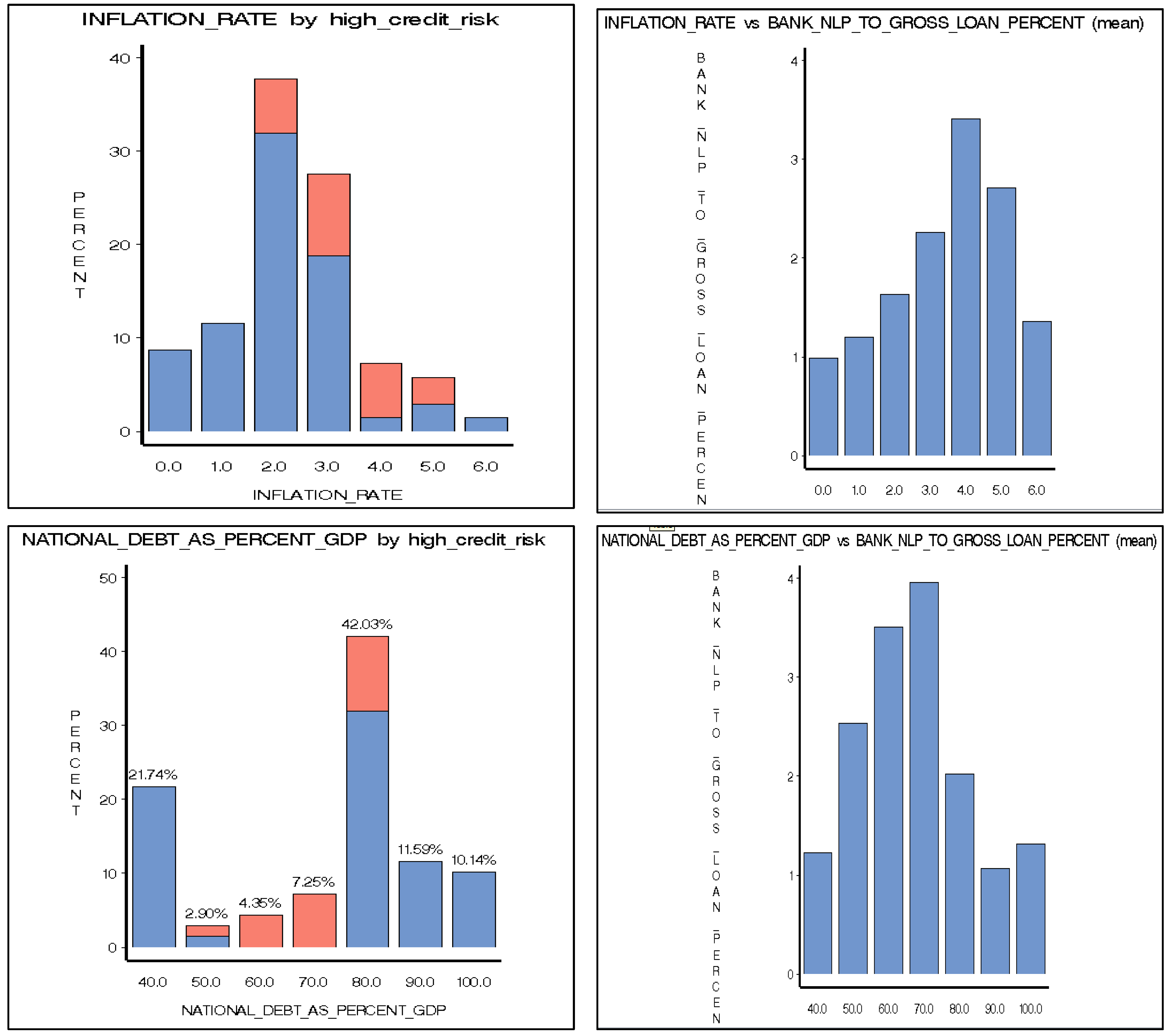
| Inflation rate | Overall increase in prices and increase in the cost of living | INFLATION_RATE | Independent variable | It demonstrates the buying power of money and is a primary macroeconomic predictor of NPLs. The existing literature contains inconsistent, contrary findings about the positive or negative impacts of inflation on NPLs. This highlights a gap and demands additional in-depth research. | [16,17,23,25] |
| National debt as percent of GDP | Ratio of country’s public debt to its GDP | NATIONAL_DEBT_AS_PERCENT_GDP | Independent variable | It can create global and/or domestic market panic when it arises. Multiple empirical investigations present a high association pattern between two economic crises, where bank failures are typically preceded by uncontrolled national indebtedness. | [2,10,11] |
| Logistic Regression | Neural Network | Decision Tree |
|---|---|---|
| Finance scholars utilize this statistical classification approach to elucidate intricate relationships among variables, gaining benefits in variable selection and coefficient shrinkage through cross-validation [34]. Logistic regression does not require a linear relationship between the response and predictor variable but the former must be categorical. The assumption of normal distribution may not always be applicable in real-world scenarios that can be characterized by non-linear data and correlated variables [35,36]. Consequently, this study also considers nonparametric models that do not rely on assumptions about data distribution. | Neural networks are becoming increasingly popular among scholars in the finance domain for credit risk evaluation because they outperform in statistical features like logistic regression and optimisation approaches [37]. The opposing strand of researchers is critical of their application as it is unstable, depends on the sample, and requires extensive computation and lengthy execution periods, which makes it difficult to conclude the optimal neural network [38]. The primary benefit is their strong generalisation ability. However, they are black-box models that are difficult for humans to interpret [39]. | The most popular ML technique for predicting credit risk and identifying financial fraud is the decision tree, which is a non-parametric and supervised learning technique [40]. One empirical investigation found that because decision trees are particularly sensitive to unbalanced data, they are the perfect choice for early credit risk warning [41], where taking preventative actions months in advance to avoid potential financial losses is essential [42]. Also, decision trees are explainable and easy to interpret compared to most conventional machine learning techniques, making them appealing to non-computing disciplines such as finance and economics. |
| Research Gap | Proposed Solution |
|---|---|
| There are US-focused NPL research studies that cover different scenarios: baseline (most likely scenario—low-credit-risk zone) or economically adverse (stress scenarios—high-credit-risk zone) [17]. | This study includes a comprehensive analysis of the UK’s NPL data from 2005 to 2021 to cover various scenarios, such as baseline (most likely scenario—low-credit-risk zone) and economically adverse scenarios (stress scenarios—high-credit-risk zone). |
| Very few studies investigate national savings as the driver of credit risk, and those that do refer to data from savings banks and not the macroeconomic national savings data [10]. | This study examines the behaviour of the UK’s national savings data from the credit risk perspective. |
| Existing studies do not consider a comprehensive outlook of employment status [21]. There is a need to cover both employment and the unemployment rate simulteneously against credit risk. | This study is unique in that it examines the impact of the employment rate and unemployment rate on NPLs separately and treats the employment rate as a distinct macroeconomic indicator. |
| There is a contradictory view about the UK currency exchange rate’s impact on NPLs [27], which needs detailed investigation. | This study validates the conflicting association between the UK’s currency exchange rate and NPLs. |
| The impact of trade deficit on credit risk has not received much attention [29]; thus, there is a need to examine the effects of the UK’s trade deficits on NPLs. | This study extensively analyses the UK’s trade deficit data and NPL association. |
| The literature investigating the link between NPLs and the inflation rate has inconsistent and contrary findings about the link [16,17,23,25], which clearly demands additional in-depth investigations. | This study extensively analyses the UK’s inflationary data and NPL link. |
| There is another gap which reveals that the majority of studies only concentrate on the definition of risk (potential loss value or uncertainty of outcome) [9]. | This study integrates a binary target variable while retaining the original numeric target variable to cater both aspects of risk, estimating real credit risk value and the probability. |
| While there are numerous studies, as examined in the literature review section, on econometrics and big data analytics, very few address problem solution by combining the knowledge of banking, finance industry expertise, and advanced analytics. | This study implements advanced analytics such as predictive, descriptive, diagnostic, trend analysis, and the correlation of each study variable from the banking and finance industry. This research not only supplements but mitigates the strengths and weaknesses of both targeted domains. Thus, this research delivers an excellent blend of advanced analytics and banking–finance domain expertise. |
| Variable | Information Value |
|---|---|
| INFLATION_RATE | 3.3035 |
| NET_NATIONAL_INCOME | 2.1769 |
| EMPLOYMENT_RATE | 1.9857 |
| GBP_USD_EXCHANGE_RATE | 1.5367 |
| UNEMPLOYMENT_RATE | 1.5291 |
| NATIONAL_DEBT_AS_PERCENT_GDP | 1.1663 |
| NATIONAL_SAVINGS | 0.8671 |
| GDP_QTQ_GROWTH_RATE | 0.8505 |
| TOTAL_TRADE_DEFICIT | 0.7545 |
| Variable | VIF |
|---|---|
| NET_NATIONAL_INCOME | 29.77 |
| NATIONAL_SAVINGS | 14.35 |
| EMPLOYMENT_RATE | 88.08 |
| UNEMPLOYMENT_RATE | 53.91 |
| GDP_QTQ_GROWTH_RATE | 1.88 |
| GBP_USD_EXCHANGE_RATE | 4.61 |
| TOTAL_TRADE_DEFICIT | 1.45 |
| INFLATION_RATE | 1.65 |
| NATIONAL_DEBT_AS_PERCENT_GDP | 11.7 |
| Correlation Coefficient Range | Interpretation | Correlations Pairs with Correlation Coefficient |
|---|---|---|
| 0.9 to 1.0 | positive and a very strong correlation | NET_NATIONAL_INCOME—NATIONAL_SAVINGS (0.9289) |
| 0.3 to 0 | positive and a very weak (low) or negligible correlation | GDP_QTQ_GROWTH_RATE—GBP_USD_EXCHANGE_RATE (0.1464) |
| −1 to −0.9 | negative and a very strong correlation | EMPLOYMENT_RATE—UNEMPLOYMENT_RATE (−0.9466) |
| Covariance Matrix | |
|---|---|
| NATIONAL_DEBT_AS_PERCENT_GDP | |
| GBP_USD_EXCHANGE_RATE | −3.772 |
| Model Description | Model Equation |
|---|---|
| Backward_Regression | HIGH_CREDIT_RISK = −40.1049 + 1.2648 (INFLATION_RATE) − 0.3805 (NATIONAL_DEBT_PERCENT_GDP) + 0.000514 (NATIONAL_SAVINGS) − 0.00021 (NATIONAL_INCOME) − 0.00117 (TOTAL_TRADE_DEFICIT) + 10.7913 (UNEMPLOYMENT_RATE) |
| Stepwise_Regression | HIGH_CREDIT_RISK = −34.24 + 4.6830 (UNEMPLOYMENT_RATE) |
| Forward_Regression | HIGH_CREDIT_RISK = −34.24 + 4.6830 (UNEMPLOYMENT_RATE) |
| Variable | Weight |
|---|---|
| UNEMPLOYMENT_RATE | 1.285231083 |
| NATIONAL_SAVINGS | 0.732948287 |
| INFLATION_RATE | 0.237606653 |
| TOTAL_TRADE_DEFICIT | −0.01663233 |
| GDP_QTQ_GROWTH_RATE | −0.03683999 |
| NET_NATIONAL_INCOME | −0.28950698 |
| NATIONAL_DEBT_AS_PERCENT_GDP | −0.95127149 |
| GBP_USD_EXCHANGE_RATE | −1.48455938 |
| EMPLOYMENT_RATE | −1.51530151 |
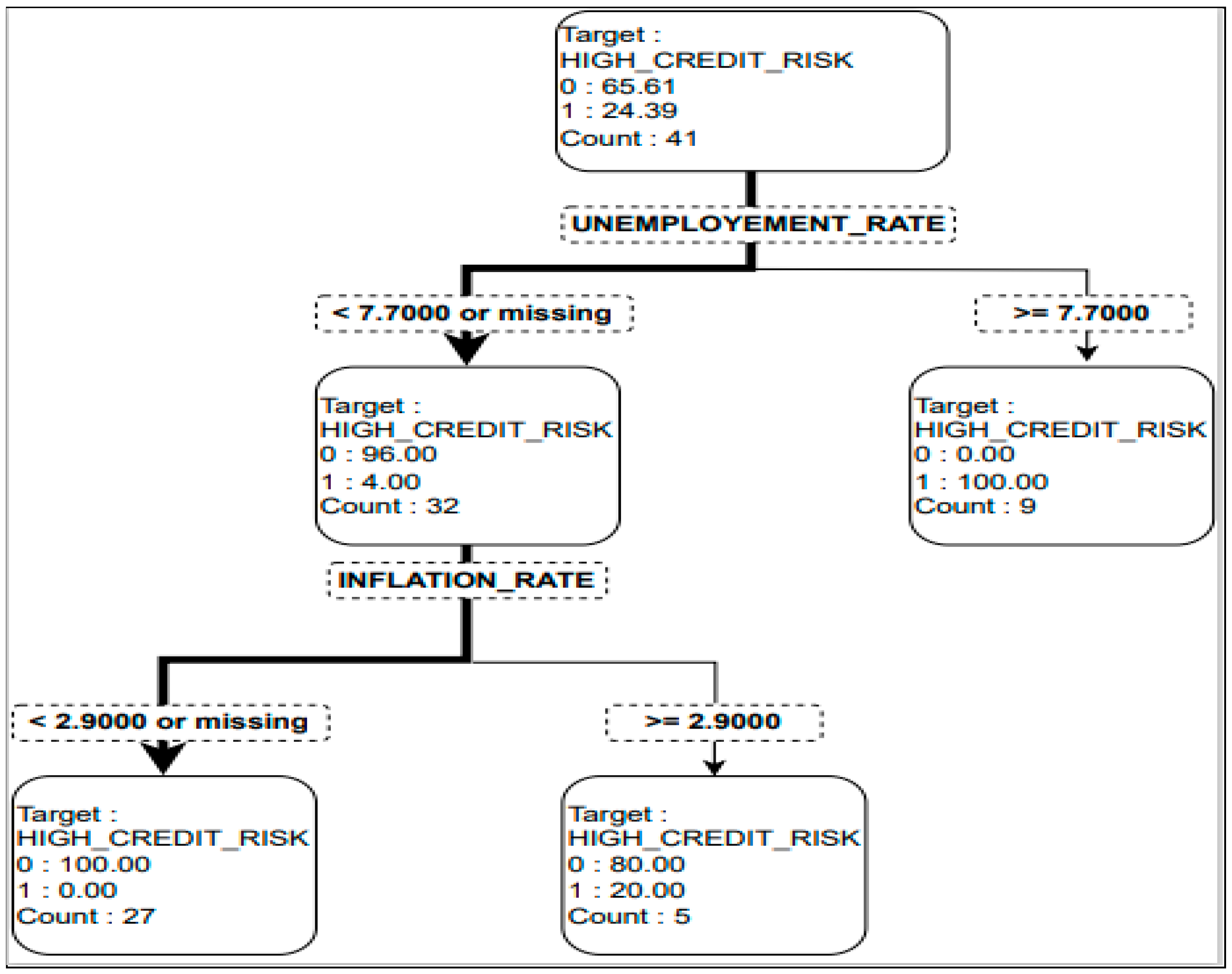
| Interpretation of Decision Tree |
|---|
| 1. If the unemployment rate in the UK exceeds 7.7, then there is a 100% chance of high credit risk—represented by 1. |
| 2. If the UK’s unemployment rate is less than 7.7, which implies that it is not unmanageable, then there is around a 4% chance of high credit risk—represented by 1. |
| 3. If the UK’s unemployment rate is less than 7.7 but the quarterly inflation rate exceeds 2.9, then there is a 20% chance of high credit risk—represented by 1. |
| 4. If the inflation rate in the UK remains less than 2.9, then there is no chance of high credit risk. |
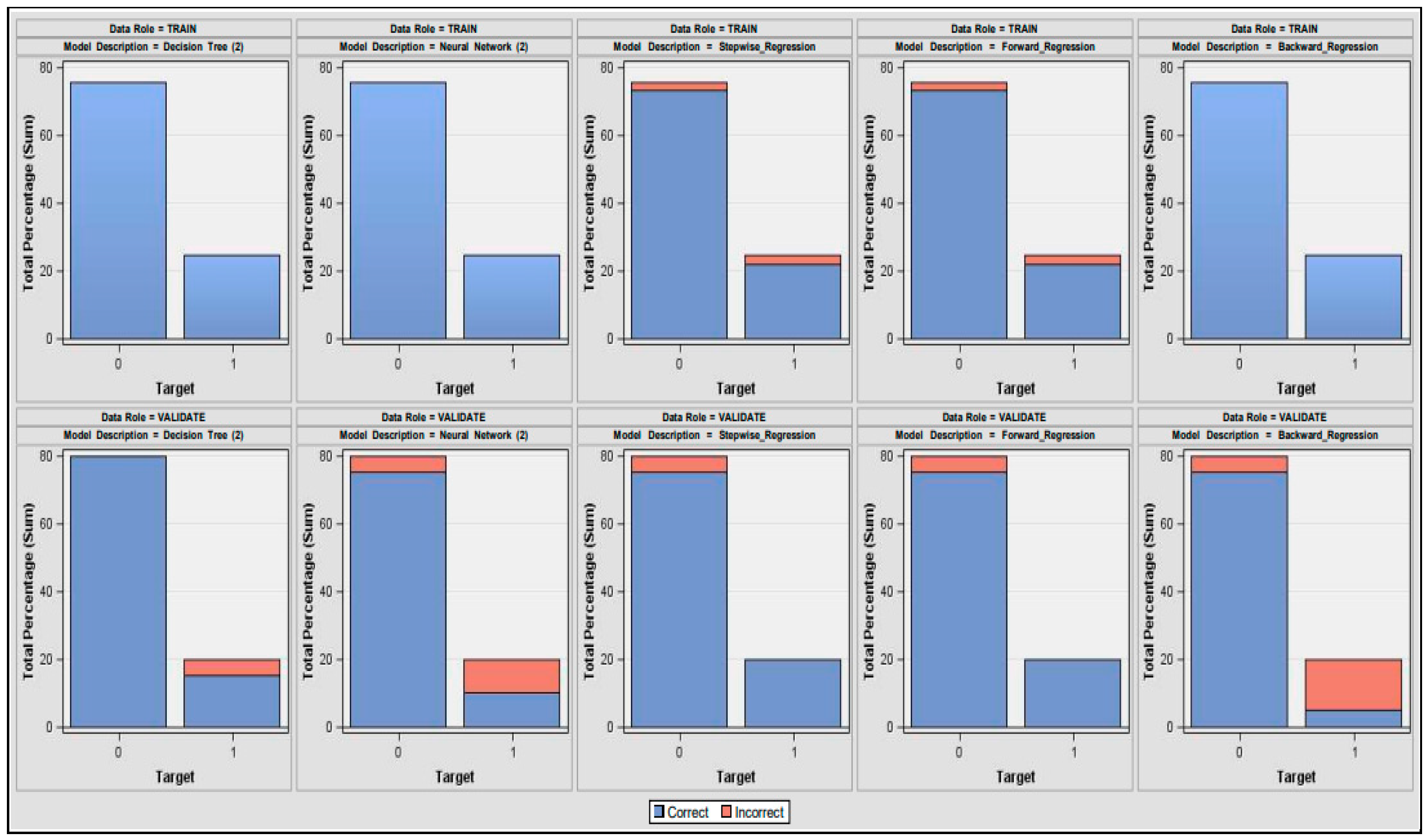
| Model Node | Data Model | Recall | Precision | Sensitivity | Specificity | Accuracy |
|---|---|---|---|---|---|---|
| Tree2 | Decision_Tree | 0.75 | 1 | 0.75 | 1 | 0.95 |
| Neural2 | Neural_Network | 0.5 | 0.67 | 0.5 | 0.93 | 0.85 |
| Reg2 | Stepwise_Regression | 0.8 | 0.8 | 0.8 | 0.93 | 0.90 |
| Reg3 | Forward_Regression | 0.8 | 0.8 | 0.8 | 0.93 | 0.90 |
| Reg4 | Backward_Regression | 0.25 | 0.5 | 0.25 | 0.93 | 0.80 |
| Performance Measures | Interpretation |
|---|---|
| Precision | The decision tree has the greatest precision, suggesting the generation of more relevant results than irrelevant ones. |
| Recall | Among all models, stepwise and forward regression models exhibit high recall scores. |
| Accuracy | When compared to the other models, the decision tree has the highest accuracy of 95%. The accuracy of the backward regression model is lowest due to the large number of predictor variables in the model equation. Accuracy has one limitation to deliver the best results for balanced data [62]. Thus, we assess two more additional performance indicators: sensitivity and specificity. |
| Sensitivity | Forward and stepwise logistic regression models are more sensitive to outliers than the other models, making them less robust to extreme values than decision trees, which do not divide trees based on outliers [63]. |
| Specificity | Inflation rate and unemployment rate are the most specific to the high-credit-risk zone. |
Disclaimer/Publisher’s Note: The statements, opinions and data contained in all publications are solely those of the individual author(s) and contributor(s) and not of MDPI and/or the editor(s). MDPI and/or the editor(s) disclaim responsibility for any injury to people or property resulting from any ideas, methods, instructions or products referred to in the content. |
© 2024 by the authors. Licensee MDPI, Basel, Switzerland. This article is an open access article distributed under the terms and conditions of the Creative Commons Attribution (CC BY) license (https://creativecommons.org/licenses/by/4.0/).
Share and Cite
Sharma, H.; Andhalkar, A.; Ajao, O.; Ogunleye, B. Analysing the Influence of Macroeconomic Factors on Credit Risk in the UK Banking Sector. Analytics 2024, 3, 63-83. https://doi.org/10.3390/analytics3010005
Sharma H, Andhalkar A, Ajao O, Ogunleye B. Analysing the Influence of Macroeconomic Factors on Credit Risk in the UK Banking Sector. Analytics. 2024; 3(1):63-83. https://doi.org/10.3390/analytics3010005
Chicago/Turabian StyleSharma, Hemlata, Aparna Andhalkar, Oluwaseun Ajao, and Bayode Ogunleye. 2024. "Analysing the Influence of Macroeconomic Factors on Credit Risk in the UK Banking Sector" Analytics 3, no. 1: 63-83. https://doi.org/10.3390/analytics3010005
APA StyleSharma, H., Andhalkar, A., Ajao, O., & Ogunleye, B. (2024). Analysing the Influence of Macroeconomic Factors on Credit Risk in the UK Banking Sector. Analytics, 3(1), 63-83. https://doi.org/10.3390/analytics3010005