Two Unitary Quantum Process Tomography Algorithms Robust to Systematic Errors ^†

Abstract

Quantum process tomography (QPT) methods aim at identifying a given quantum process. QPT is a major quantum information processing tool, since it especially allows one to characterize the actual behavior of quantum gates, which are the building blocks of quantum computers. The present paper focuses on the estimation of a unitary process. This class is of particular interest because quantum mechanics postulates that the evolution of any closed quantum system is described by a unitary transformation. Unitary processes have significantly fewer parameters than general quantum processes ($2^{2n_{qb}}$ vs. $2^{4n_{qb}}-2^{2n_{qb}}$ real independent parameters for $n_{qb}$ qubits). By assuming that the process is unitary we develop two methods that scale better with the size of the system. In the present paper, we stay as close as possible to the standard setup of QPT: the operator has to prepare copies of different input states. The properties those states have to satisfy in order for our method to achieve QPT are very mild. Therefore, we choose to operate with copies of $2^{n_{qb}}$ initially unknown pure input states. In order to perform QPT without knowing the input states, we perform measurements on half the copies of each state, and let the other half be transformed by the system before measuring them (each copy is only measured once). This setup has the advantage of removing the issue of systematic (i.e., same on all the copies of a state) errors entirely because it does not require the process input to take predefined values. We develop a straightforward analytical solution that first estimates the states from the averaged measurements and then finds the unitary matrix (representing the process) coherent with those estimates by using our analytical solution to an extended version of Wahba’s problem. This estimate may then be used as an initial point for a fine tuning algorithm that maximizes the likelihood of the measurements. Simulation results show the effectiveness of the proposed methods.

1. Prior Work and Problem Statement

System identification and system inversion are well-known problems, especially for classical systems. These problems are less challenging in the “nonblind”/“supervised” case [1] where the aim is, e.g., to identify the considered system by using the known input and the measured output. In contrast, in the “blind”/“unsupervised” case [2], the input values are unknown and uncontrolled, but some hypotheses are sometimes made on the input signal(s).

For quantum systems, non-blind system identification methods were first introduced in 1997 in [3] that came up with the name quantum process tomography (QPT), see [4]. They use copies of a set of known pure input states that are transformed by the process. Those transformed states are then measured and estimated using quantum state tomography (QST aims at estimating a quantum state using measurements). From there, the parameters of the process can be estimated from what is essentially a regression. This method scales poorly when the number of qubits increases, and is only experimentally feasible for one or two qubits. This is to be expected because, in general, a quantum process has $d^4-d^2$ independent real parameters ([4], p. 391), with d the dimension of the Hilbert space (for an $n_{qb}$-qubit system $d=2^{n_{qb}}$). This method would later be called standard QPT (SQPT), in contrast to non-standard QPT that uses ancilla qubits and weak measurements (see [5] for a survey). In Ref. [6], a SQPT approach that scales better with the number of qubits by assuming that the process is sparse is introduced. Like Baldwin et al., in most of [7], we choose to restrict ourselves to unitary processes. This class is of particular interest because the evolution of any closed quantum system is described by a unitary transformation. A unitary process has $d^2$ independent real parameters.

A significant problem of SQPT is the need to precisely prepare the copies of the input states. Any systematic error on the input state has huge consequences for the precision. In 2015, we introduced the blind version of QPT (BQPT) in [8], then detailed it in [9], and more recently in [10]. In those papers, we focused on the tomography of the two-qubit cylindrical-symmetry Heisenberg coupling process. For those algorithms, the operator has to prepare one or several copies of an unknown set of initial states. This requires a preparation procedure to be known and reproducible, so that several copies of each used state may be prepared. It is not a violation of the no cloning theorem, the latter does not apply if we prepared the state that we want to reproduce. This idea removes the issue of systematic errors (with respect to a desired state) during the preparation. The system is identified by processing output measurements associated with $n_s$ different unknown input states going through the system. Generally, we need to perform QST or at least to estimate some measurement outcome probabilities for each of the $n_s$ output states. For the approaches of [8,9], this kind of QST requires $n_c$ copies of each considered output state. Therefore, for each one of the $n_s$ states the same experiment has to be repeated $n_c$ times with the same input state value, for $n_s\times n_c$ input state preparations in total. The most recent paper [10] also proposes “single-preparation BQPT methods” (SBQPT), i.e., methods which can operate with only one instance of each considered input state, $n_c=1$.

In [11] (2021), we introduced the setup that will be further developed in the current paper. In Ref. [11] we considered copies of a single 2-qubit state (initially unentangled) being transformed by a unitary process and measured at 5 different time delays (${\Delta }_t,....,5{\Delta }_t$). In the current paper, we consider a setup closer to standard QPT where only two times are considered (see Figure 1). The unit-norm d-dimensional vectors ${\mathbf{v}}_1,...,{\mathbf{v}}_d$ represent the initial quantum pure states. Those initial states are considered unknown. We simply assume that they are pure, unentangled, linearly independent, and that at least one of the states is not orthogonal to all the others (i.e., $\exists j\mathrm{such}\mathrm{that}\forall k\ne j{\mathbf{v}}_j/\perp {\mathbf{v}}_j$). These are reasonable hypotheses, as long as the qubits are prepared separately, the states are unentangled; and d random states are always (probability 1) linearly independent and not orthogonal in the d-dimensional Hilbert space. After waiting ${\Delta }_t$, each input state vector ${\mathbf{v}}_j$ is multiplied by the unitary $d\times d$ matrix $\mathbf{M}$, thus yielding the output state ${\mathbf{w}}_j=\mathbf{M}{\mathbf{v}}_j$.

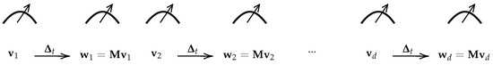
Figure 1. Considered setup.

We assume that enough types of measurements are performed on copies of all $2d$ states to achieve QST on each state. The present paper does not focus on the measurements performed and the QST algorithm. We simply assume that each state is recovered up to a global phase and a low residual error. For the numerical simulations, we will use the first QST algorithm of [12] which is suited to pure states and has the advantage of only requiring unentangled measurements on each qubit. However, the current paper is not bound to [12] and any pure state QST algorithm [13,14] can be performed. The fact that we perform measurements on the input states means that our algorithm is not blind, but since their values are not imposed by the proposed method, we keep the main advantage of the blind approaches (resilience to systematic error).

Section 2 briefly describes the system states and measurements. Section 3 describes a straightforward method that does not require an initialization and achieves QPT using the estimates of the states. Section 4 describes a method that improves the first estimate by maximizing the likelihood of the measurements. Finally, Section 5 contains some numerical results.

2. States and Measurements

2.1. Considered States

We hereafter consider an $n_{qb}$-qubit system, typically composed of distinguishable spins 1/2. Any pure state $|\phi ⟩$ of that system is here expressed in the basis defined as the tensor product of the standard bases associated with each qubit. The components of $|\phi ⟩$ in that basis can be stored in a d-element vector $\mathbf{v}$, with $d=2^{n_{qb}}$. The components of $\mathbf{v}$ are complex and the norm of $\mathbf{v}$ is 1. The global phase of $|\phi ⟩$ has no physical meaning, so we can assume that the first non-zero component of $\mathbf{v}$ is a real strictly positive number. In the rest of the paper, we consider the vector $\mathbf{v}$ instead of the state $|\phi ⟩$.

2.2. Considered Types of Measurements

First focusing on a single qubit, we perform measurements based on the three Pauli operators ${\sigma }_x,{\sigma }_y$, and ${\sigma }_z$ [4] and, e.g., related to spin 1/2 components along the $X,Y$, and Z axes. For each such direction, we define the eigenvector matrix whose first and second columns are the eigenvectors of the considered Pauli operator, respectively, associated with eigenvalues $+1$ and $-1$ in the standard basis. These eigenvector matrices may be shown to read:

$${\mathbf{P}}_X=\frac{1}{\sqrt{2}}\left(\begin{array}{cc}1& 1\\ 1& -1\end{array}\right){\mathbf{P}}_Y=\frac{1}{\sqrt{2}}\left(\begin{array}{cc}1& 1\\ i& -i\end{array}\right){\mathbf{P}}_Z=\left(\begin{array}{cc}1& 0\\ 0& 1\end{array}\right).$$

(1)

The probabilities of the outcomes $+1$ and $-1$ when performing a measurement for state $\mathbf{v}$ along $\mathcal{D}\in \{X,Y,Z\}$ are, respectively, the first and second elements of $|{{\mathbf{P}}_{\mathcal{D}}}^{†}{\mathbf{v}|}^2$ where ${|.|}^2$ is the element-wise squared modulus and ${.}^{†}$ is the trans conjugate.

When considering $n_{qb}$ qubits, we perform the above-defined measurements in parallel for all qubits. Each such type $\mathcal{T}$ of measurements corresponds to a given direction ${\mathcal{D}}_m\in \{X,Y,Z\}$ for the m-th qubit for each m in $\{1,...,n_{qb}\}$ ($\mathcal{T}={\mathcal{D}}_1...{\mathcal{D}}_{n_{qb}}$). For each set of eigenvectors ${\mathbf{e}}_1,...,{\mathbf{e}}_{n_{qb}}$ (each ${\mathbf{e}}_m$ is a column of one of the matrix of ${\mathbf{P}}_{{\mathcal{D}}_m}$ of (1)) and eigenvalue $a_1,...,a_{n_{qb}}$ ($a_m$ is either $+1$ if ${\mathbf{e}}_m$ is the first column of ${\mathbf{P}}_{{\mathcal{D}}_m}$ and $-1$ if it is the second), respectively, associated with each qubit, the probability that a measurement on $\mathbf{v}$ yields these eigenvalues reads: $p_{a_1...a_{n_{qb}}}={\left|{({\mathbf{e}}_1\otimes ....\otimes {\mathbf{e}}_{n_{qb}})}^{†}\mathbf{v}\right|}^2$ (where ⊗ is the tensor product). Those d probabilities (from $p_{+1...+1}$ to $p_{-1...-1}$) therefore form the vector $|{\mathbf{P}}_{\mathcal{T}}^{†}{\mathbf{v}|}^2$ where ${\mathbf{P}}_{\mathcal{T}}$ is the eigenvector matrix associated with the measurement along the directions ${\mathcal{D}}_1...{\mathcal{D}}_{n_{qb}}$ of $\mathcal{T}$. It is expressed as the tensor (i.e., Kronecker) product of one-qubit matrices of (1)

$${\mathbf{P}}_{\mathcal{T}}=\underset{m=1}{\overset{n_{qb}}{⨂}}{\mathbf{P}}_{{\mathcal{D}}_m}\mathrm{with}{\mathcal{D}}_m\in \{X,Y,Z\}\mathrm{s}.\mathrm{t}.\mathcal{T}={\mathcal{D}}_1...{\mathcal{D}}_{n_{qb}}.$$

(2)

For example with $n_{qb}=2$ qubits, measuring the first one along ${\mathcal{D}}_1=Z$ and the second one along ${\mathcal{D}}_2=X$ ($\mathcal{T}=ZX$) yields the following eigenvector matrix ${\mathbf{P}}_{\mathcal{T}}={\mathbf{P}}_Z\otimes {\mathbf{P}}_X=\frac{1}{\sqrt{2}}\left(\begin{array}{cccc}1& 1& 0& 0\\ 1& -1& 0& 0\\ 0& 0& 1& 1\\ 0& 0& 1& -1\end{array}\right)$. Those measurements are not multi-qubit Pauli measurements (used in (8.149) in [4]) because the latter only have 2 outcomes whereas the former have d outcomes (they are the concatenations of $n_{qb}$ 2-outcome measurements). In the rest of the paper, this type of measurement will be referred to as a string of $X,Y$, and Z (in this example, $\mathcal{T}=ZX$).

For $n_{qb}$ qubits, there are $3^{n_{qb}}$ of those measurements. Since we are dealing with pure states, we can work with only 4 types of measurements: ${\mathcal{T}}_1=Z...Z,{\mathcal{T}}_2=Y...Y,{\mathcal{T}}_3=X...X,{\mathcal{T}}_4=XY...$ (${\mathcal{T}}_4$ is X on every odd numbered qubit and Y on the even numbered, all the others are the same measurement types on all qubits). In Ref. [12] we explain how to perform QST with those measurements in Section 3 and Section 5. We will not mention it again in the rest of the paper, but if $n_{qb}=1$ we perform 3 types of measurements instead of 4 (along directions X, Y, and Z), as ${\mathcal{T}}_4={\mathcal{T}}_3=X$.

Those measurements are performed on ${\left\{{\mathbf{v}}_j\right\}}_{j\in \{1,...,d\}}$ and ${\left\{{\mathbf{w}}_j\right\}}_{j\in \{1,...,d\}}$. In total, $2d$ states are measured with 4 types of measurements. To estimate probabilities, each measurement is performed a given number of times that we call $n_c$, the total number of measurements performed is $8d{n}_c$. For each one of the $8d$ distinct measurements, the numbers of times each one of the d outcomes was observed are stored in the d-dimensional vector ${\mathbf{n}}_{j,k,\ell }$ where $j\in \{1,...,d\}$ is the index if the measured state, $k\in \{1,2,3,4\}$ defines the type of the measurement and $l\in \{0,1\}$ is 0 if ${\mathbf{v}}_j$ is measured and 1 if it is ${\mathbf{w}}_j$. Thus, ${\mathbf{n}}_{j,k,\ell }$ contains the measurement counts for the state ${\mathbf{M}}^{\ell }{\mathbf{v}}_j$ along direction ${\mathcal{T}}_k$. The expected value of ${\mathbf{n}}_{j,k,\ell }$ is $n_c{\left|{\mathbf{P}}_{{\mathcal{T}}_k}^{†}{\mathbf{M}}^{\ell }{\mathbf{v}}_j\right|}^2$.

3. QST-Based Solution

3.1. Main Idea

We assume that QST is performed properly for the states of Figure 1. It yields:

$$\widehat{{\mathbf{v}}_j}={\mathbf{v}}_j.e^{i{\xi }_j^v}+{\mathit{\epsilon }}_j^{QST}\forall j\in \{1,...,d\}\mathrm{and}\widehat{{\mathbf{w}}_j}={\mathbf{w}}_j.e^{i{\xi }_j^w}+{\mathit{\epsilon }}_{d+j}^{QST}\forall j\in \{1,...,d\}$$

where ${\xi }_j^v$ and ${\xi }_j^w$ are unknown phases and ${\epsilon }_j^{QST}$ is the residual error, such that $E\left(\right||{\epsilon }_j^{QST}{\left|\right|}_2)\underset{n_c\to +\infty }{⟶}0$ (E is the expected value). For the rest of this section, we consider ${\epsilon }_j^{QST}=0$ unless stated otherwise. In Section 2.1, we stated that the global phases of the states do not matter. This is true if the states are considered independently and this is the reason why the QST cannot recover the global phase. However, when the states are considered together (in order to find $\mathbf{M}$) the differences between the global phases of the different states matter.

We know that ${\mathbf{w}}_j=\mathbf{M}{\mathbf{v}}_j\forall j\in \{1,...,d\}$, therefore, with ${\xi }_j={\xi }_j^v-{\xi }_j^w\forall j$, we have: $e^{i{\xi }_j}\widehat{{\mathbf{w}}_j}=\mathbf{M}\widehat{{\mathbf{v}}_j}\forall j\in \{1,...,d\}$. Changing $\mathbf{M}$ to $\mathbf{M}.e^{-i{\xi }_1}$ and ${\xi }_j$ to ${\xi }_j-{\xi }_1\forall j\in \{1,...,d\}$ does not change the equality, so we can also assume ${\xi }_1=0$ and accept that $\mathbf{M}$ can only be recovered up to a global phase.

In the next section, we explain how to estimate the other phases $e^{i\widehat{{\xi }_j}}\forall j\in \{2,...,d\}$. From that, we can define $\widetilde{{\mathbf{w}}_j}=\widehat{{\mathbf{w}}_j}.e^{i\widehat{{\xi }_j}}$ with which an estimate of $\mathbf{M}$ can easily be found as the problem becomes:

$$\widetilde{{\mathbf{w}}_j}=\mathbf{M}\widehat{{\mathbf{v}}_j}\forall j\in \{1,...,d\}.$$

(3)

$\widehat{\mathbf{M}}=[\widetilde{{\mathbf{w}}_1},...,\widetilde{{\mathbf{w}}_d}]{[\widehat{{\mathbf{v}}_1},...,\widehat{{\mathbf{v}}_d}]}^{-1}$ works as a solution. However, it is generally not a unitary solution because of the QST errors. Finding $\widehat{\mathbf{M}}\in {\mathbb{U}}_3\left(\mathbb{R}\right)$ that is the least square solution of $\widehat{{\mathbf{a}}_j}=\mathbf{M}\widehat{{\mathbf{b}}_j}\forall j\in \{1,...,n\}$ with $\widehat{{\mathbf{a}}_j},\widehat{{\mathbf{b}}_j}\in {\mathbb{R}}^3$ is a well known problem in the aerospace community. It is called Wahba’s problem after Wahba who first posed it in 1965 [15]. We have adapted its solution for $\mathbf{M}\in {\mathbb{U}}_d\left(\mathbb{C}\right)$ (details will be provided in a future paper). This yields:

$$\mathbf{B}=[\widetilde{{\mathbf{w}}_1},...,\widetilde{{\mathbf{w}}_d}]{[\widehat{{\mathbf{v}}_1},...,\widehat{{\mathbf{v}}_d}]}^{†}⟶\mathbf{B}=\mathbf{U}\mathbf{S}{\mathbf{V}}^{†}⟶{\widehat{\mathbf{M}}}_{LS}=\mathbf{U}{\mathbf{V}}^{†}$$

(4)

where $\mathbf{U}\mathbf{S}{\mathbf{V}}^{†}$ is the singular value decomposition of $\mathbf{B}$. We showed that this solution is optimal in the least square (LS) sense. The solution is unique if, and only if, both $\left[\widehat{{\mathbf{v}}_1},...,\widehat{{\mathbf{v}}_d}\right]$ and $[\widetilde{{\mathbf{w}}_1},...,\widetilde{{\mathbf{w}}_d}]$ are of full rank. This QPT method can be extended to any higher number of input states but with fewer than d, the solution is not unique.

3.2. Phase Recovery

The aim of the current section is to find $e^{i\widehat{{\xi }_j}}\forall j\in \{2,...,d\}$ given the vectors, $\widehat{{\mathbf{v}}_j},\widehat{{\mathbf{w}}_j}\forall j\in \{1,...,d\}$ such that there exist a unitary matrix $\mathbf{M}$ that realizes (3), with ${\xi }_1$ assumed to be 0.

The basic idea is to use the fact that $e^{i{\xi }_{j_1}}\widehat{{\mathbf{w}}_{j_1}}+e^{i{\xi }_{j_2}}\widehat{{\mathbf{w}}_{j_2}}=\mathbf{M}(\widehat{{\mathbf{v}}_{j_1}}+\widehat{{\mathbf{v}}_{j_2}})\forall j_1,j_2\in \{1,...,d\}$ and $\mathbf{M}$ is unitary so does not change the norm. Therefore, ${\xi }_{j_1,j_2}={\xi }_{j_2}-{\xi }_{j_1}$ is subject to:

$$\begin{array}{c}\parallel \widehat{{\mathbf{w}}_{j_1}}+e^{i{\xi }_{j_1,j_2}}\widehat{{\mathbf{w}}_{j_2}}{\parallel }_2^2={\parallel \widehat{{\mathbf{v}}_{j_1}}+\widehat{{\mathbf{v}}_{j_2}}\parallel }_2^2\\ \iff \parallel \widehat{{\mathbf{w}}_{j_1}}{\parallel }_2^2+\parallel \widehat{{\mathbf{w}}_{j_2}}{\parallel }_2^2+r_{j_1,j_2}cos\left({\xi }_{j_1,j_2}\right)+i_{j_1,j_2}sin\left({\xi }_{j_1,j_2}\right)={\parallel \widehat{{\mathbf{v}}_{j_1}}+\widehat{{\mathbf{v}}_{j_2}}\parallel }_2^2\end{array}$$

(5)

with $r_{j_1,j_2}$ and $i_{j_1,j_2}$ the real and imaginary part of $2{\widehat{{\mathbf{w}}_{j_2}}}^{†}\widehat{{\mathbf{w}}_{j_1}}$, respectively. Equation (5) is solvable if, and only if, $\widehat{{\mathbf{w}}_{j_1}}$ and $\widehat{{\mathbf{w}}_{j_2}}$ are not orthogonal. By writing $cos\left({\xi }_{j_1,j_2}\right)=\frac{1-t^2}{1+t^2}$ and $sin\left({\xi }_{j_1,j_2}\right)=\frac{2t}{1+t^2}$ with $t=tan\left(\frac{{\xi }_{j_1,j_2}}{2}\right)$, (5) becomes a quadratic equation (when both sides are multiplied by $1+t^2$) with two real solutions for t, corresponding to two solutions for ${\xi }_{j_1,j_2}$ that we call ${\xi }_{j_1,j_2}^1$ and ${\xi }_{j_1,j_2}^2$ (they can have the same value). It is numerically possible to have no real solution but this never happens if there are no QST errors. If there are no real solutions, we consider ${\xi }_{j_1,j_2}^1$ and ${\xi }_{j_1,j_2}^2$ both set to the real part of the complex solutions.

In order to choose between ${\xi }_{j_1,j_2}^1$ and ${\xi }_{j_1,j_2}^2$, we have to consider a third pair of vectors: $\{\widehat{{\mathbf{v}}_{j_3}},\widehat{{\mathbf{w}}_{j_3}}\}$. Solving (5) for the 3 possible pairs of indices ($\{j_1,j_2\},\{j_1,j_3\},\{j_2,j_3\}$) gives us $2^3=8$ possibilities for ${\xi }_{j_1,j_2}$, ${\xi }_{j_1,j_3}$, ${\xi }_{j_2,j_3}$. However, by definition ${\xi }_{j_2,j_3}={\xi }_{j_1,j_3}-{\xi }_{j_1,j_2}$ and it may be hoped that there is only one of the 8 possibilities that satisfies this. We keep the solution that comes the closest.

We can apply this method for $(j_1,j_2,j_3)\in \{(1,2,3),(3,4,5)$$,...,(d-2,d-1,d)\}$. We would thus know all the differences between the phases, and, since ${\xi }_1$ is 0, we would know all the phases.

In practice, doing this would work as long as one of the ${\mathbf{v}}_j$ is not orthogonal to all the others (otherwise (5) is not solvable for enough indices $j_1,j_2$); but this would not be robust to a realistic QST error. The actual algorithm we use will be described in a future longer paper. It is based on the same idea: finding the two solutions of (5) for all $\{j_1,j_2\}$ indices. We improve the robustness by considering more than 3 pairs of well chosen indices.

4. Fine Tuning

4.1. Problem Statement

Section 3 describes a method to achieve QPT using the results of the QST on every state. The current section details a different approach that requires an initial estimate of $\mathbf{M}$ (we will use ${\widehat{\mathbf{M}}}_{LS}$ from (4)) and finds the unitary matrix ${\widehat{\mathbf{M}}}_{ML}$ and initial states ${\widehat{\mathbf{V}}}_{ML}=[\widehat{{\mathbf{v}}_1},...,\widehat{{\mathbf{v}}_d}]$ that maximize the likelihood of the measurements. Formally: $({\widehat{\mathbf{M}}}_{ML},{\widehat{\mathbf{V}}}_{ML}=\underset{\mathbf{M},\mathbf{V}}{argmax}\mathcal{L}(\mathbf{M},\mathbf{V},\mathcal{M})$, where $\mathcal{M}={\left\{{\mathbf{n}}_{j,k,\ell }\right\}}_{j,k,\ell }$ represents the measurements results and $\mathcal{L}$ is the log-likelihood which we maximize in order to maximize the likelihood. The problem is actually simpler if we perform the maximization successively, i.e., find the best $\mathbf{V}$ for each $\mathbf{M}$ of which we compute the likelihood, ${\widehat{\mathbf{M}}}_{ML}=\underset{\mathbf{M}}{argmax}\left(\underset{\mathbf{V}}{max}\mathcal{L}(\mathbf{M},\mathbf{V},\mathcal{M})\right)$, because optimizing $\mathbf{V}$ knowing $\mathbf{M}$ (i.e., computing ${\displaystyle \underset{\mathbf{V}}{max}}\mathcal{L}(\mathbf{M},\mathbf{V},\mathcal{M})$) can be performed independently on all the ${\mathbf{v}}_j$: ${\displaystyle \underset{\mathbf{V}}{max}}\mathcal{L}(\mathbf{M},\mathbf{V},\mathcal{M})={\sum }_{j=1}^d{\displaystyle \underset{{\mathbf{v}}_j}{max}}\left(\mathcal{L}({\mathbf{v}}_j,{\mathcal{M}}_{{\mathbf{v}}_j})+\mathcal{L}(\mathbf{M}{\mathbf{v}}_j,{\mathcal{M}}_{{\mathbf{w}}_j})\right)$, where ${\mathcal{M}}_{{\mathbf{v}}_j}={\left\{{\mathbf{n}}_{j,k,0}\right\}}_k$ and ${\mathcal{M}}_{{\mathbf{w}}_j}={\left\{{\mathbf{n}}_{j,k,1}\right\}}_k$ are the measurements performed on ${\mathbf{v}}_j$ and ${\mathbf{w}}_j$, respectively. This is the case because the $\{{\mathcal{M}}_{{\mathbf{v}}_1},{\mathcal{M}}_{{\mathbf{w}}_1},...,{\mathcal{M}}_{{\mathbf{v}}_d},{\mathcal{M}}_{{\mathbf{w}}_d}\}$ are statistically independent and involve different arguments to be maximized for different j. Considering this, the problem becomes:

$${\widehat{\mathbf{M}}}_{ML}=\underset{\mathbf{M}}{argmax}\sum _{j=1}^d\underset{{\mathbf{v}}_j}{max}\left(\mathcal{L}({\mathbf{v}}_j,{\mathcal{M}}_{{\mathbf{v}}_j})+\mathcal{L}(\mathbf{M}{\mathbf{v}}_j,{\mathcal{M}}_{{\mathbf{w}}_j})\right).$$

(6)

In order to solve (6) we first need to be able to compute the likelihood of the measurements. Since most gradient based optimization algorithms can only be performed with a real number vector as argument, we also need to find real number parametrization for $\mathbf{M}$ and ${\mathbf{v}}_j$. Those two points are the focuses of the following two subsections.

4.2. Statistical Model for the Measurements

In [16], the formula for the likelihood of samples from multiple outcome measurements is given (albeit for a mixed state represented by a density matrix which we would have to replace by $\mathbf{v}{\mathbf{v}}^{†}$ or $\mathbf{w}{\mathbf{w}}^{†}$). Once we remove additive constants, the log-likelihood boils down to: $\mathcal{L}(n_1^o,...,n_d^o)={\sum }_{m=1}^d{n}_m^{o}log\left(p_m\right)$, where $p_m$ is the theoretical probabilities of the m-th outcome, and $n_m^o$ is the number of times the m-th outcome has been measured. If the measurement whose likelihood we want to compute has ${\mathbf{P}}_{{\mathcal{T}}_k}$ as eigenvectors matrix ($k\in \{1,2,3,4\}$) and is performed on ${\mathbf{v}}_j$, then ${[p_1...p_d]}^T={\left|{\mathbf{P}}_{{\mathcal{T}}_k}^{†}{\mathbf{v}}_j\right|}^2$ and ${[n_1^o...n_d^o]}^T={\mathbf{n}}_{j,k,0}$ (see the definition of ${\mathbf{n}}_{j,k,\ell }$ and ${\mathbf{P}}_{{\mathcal{T}}_k}$ in Section 2.2, ${.}^T$ stands for transpose). If, instead of $\mathbf{v}$, we measure $\mathbf{w}$, then ${[p_1...p_d]}^T={\left|{\mathbf{P}}_{{\mathcal{T}}_k}^{†}{\mathbf{w}}_j\right|}^2$ and ${[n_1^o...n_d^o]}^T={\mathbf{n}}_{j,k,1}$. Let us rewrite $\mathcal{L}$ using the notation adapted to our measurements: $\mathcal{L}({\mathbf{M}}^{\ell }{\mathbf{v}}_j,{\mathbf{n}}_{j,k,\ell })={\mathbf{n}}_{j,k,\ell }^{T}log\left(\right|{\mathbf{P}}_{{\mathcal{T}}_k}^{†}{\mathbf{M}}^{\ell }{\mathbf{v}}_j{|}^2)$ (ℓ is either 0 or 1 so ${\mathbf{M}}^{\ell }{\mathbf{v}}_j$ is either ${\mathbf{v}}_j$ or ${\mathbf{w}}_j$). We can replace $\mathcal{L}$ in (6) by its expression (knowing ${\mathcal{M}}_{{\mathbf{M}}^{\ell }{\mathbf{v}}_j}=\{{\mathbf{n}}_{j,1,\ell },...,{\mathbf{n}}_{j,4,\ell }\}$), this yields:

$${\widehat{\mathbf{M}}}_{ML}=\underset{\mathbf{M}}{argmax}\sum _{j=1}^d\underset{{\mathbf{v}}_j}{max}\sum _{k=1}^4\sum _{\ell =0}^1{n}_{j,k,\ell }^{T}log\left(|{\mathbf{P}}_{{\mathcal{T}}_k}^{†}{\mathbf{M}}^{\ell }{\mathbf{v}}_j{|}^2\right).$$

(7)

4.3. Parametrization of the Arguments

For a given $j\in \{1,...,d\}$${\mathbf{v}}_j$ represents an unentangled state. By definition, it can be decomposed as a tensor product of $n_{qb}$ 1-qubit states: ${\mathbf{v}}_j={\mathbf{q}}_{j,1}\otimes ...\otimes {\mathbf{q}}_{j,n_{qb}}$. Each ${\mathbf{q}}_{j,h},h\in \{1,...,n_{qb}\}$ has 2 real parameters, $r_{j,h}$ and ${\theta }_{j,h}$${\mathbf{q}}_{j,h}={\left[\begin{array}{cc}{r}_{j,h}& \sqrt{1-r_{j,h}^2}{e}^{i{\theta }_{j,h}}\end{array}\right]}^T$. Therefore, ${\mathbf{v}}_j$ can be parameterized with $2n_{qb}$ real parameters: ${\mathbf{v}}_j=f_{{\mathbf{v}}_j}(r_{j,1},{\theta }_{j,1},...,r_{j,n_{qb}},{\theta }_{j,n_{qb}})$.

$\mathbf{M}$ is a unitary matrix. Hence, it can be shown that there exists a Hermitian matrix $\mathbf{H}$, such that $\mathbf{M}=exp\left(i\mathbf{H}\right)$ where exp is the matrix exponential. Therefore, $\mathbf{M}$ can be parameterized with $d^2$ real parameters: $(h_1,...,h_{d^2})$, where $h_1,...,h_{d^2}$ is the parametrization of $\mathbf{H}$ starting with the $d(d+1)/2$ real parts of the components that are on or above the diagonal ($H_{1,1},H_{1,2},...,H_{d,d}$) where $H_{i_r,i_c}$ is the element on row $i_r$ and column $i_c$ of $\mathbf{H}$) and ending with the $d(d-1)/2$ imaginary parts of the components that are strictly above the diagonal ($H_{1,2},H_{1,3},...,H_{d-1,d}$). Accounting for the fact that $\mathbf{M}$ can only be recovered up to a global phase, we can assume that $h_1$ corresponding to the top left element of $\mathbf{H}$ is 0 and remove it from the parametrization. Indeed, $\mathbf{H}-h_1{\mathbf{I}}_d$ (${\mathbf{I}}_d$ is the $d\times d$ identity matrix) has a 0 for its top left element and $exp\left(i\mathbf{H}\right)$ and $exp(i\mathbf{H}-i{h}_1{\mathbf{I}}_d)$ only differ by a global phase. Therefore, as far as the optimization algorithm is concerned, $\mathbf{M}$ has $d^2-1$ real parameters: $\mathbf{M}=f_M(h_2,...,h_{d^2})$.

4.4. Optimization

In order to find the real parameters of $\mathbf{M}$ that solve (7) we use the BFGS quasi-Newton algorithm [17] initialized at the $d^2-1$ parameters that yield ${\widehat{\mathbf{M}}}_{LS}$ up to a global phase. This algorithm is implemented with the fminunc Matlab function, we provide it with the analytical expressions of the gradients of the criterion in order to make it run faster. At each step of the optimization of $\mathbf{M}$, d optimizations are performed on $2n_{qb}$ arguments in order to find the $\left\{{\mathbf{v}}_j\right\}$ (to solve the max inside the first sum in (7)). Those optimizations are also performed using the BFGS quasi-Newton algorithm with the analytical gradient provided. The latter algorithm is initialized at the real parameters of the unentangled state that is the closest to $\frac{1}{2}\widehat{{\mathbf{v}}_j}+\frac{1}{2}{\mathbf{M}}^{-1}\widetilde{{\mathbf{w}}_j}$, where ${\mathbf{M}}^{-1}$ is the inverse of the $\mathbf{M}$ at the current state of the optimization (the $\mathbf{M}$ whose likelihood we are computing in order to maximize it), j is the index of the ${\mathbf{v}}_j$ we are optimizing and $\widehat{{\mathbf{v}}_j}$ and $\widetilde{{\mathbf{w}}_j}$ are defined in Section 3.1. The optimization algorithms stop when the norm of the difference between the arguments at two successive iterations is lower than ${10}^{-30}$. Moreover, for the optimization of $\mathbf{M}$ it stops after 700 iterations if the previous criterion is not met. For 3 qubits or less, the optimization of $\mathbf{M}$ always stops before the 700 iterations. For 4 and 5 qubits, this is not always the case but the BFGS algorithm decreases the criterion at every step so even if the algorithm has not properly converged, the final estimate ${\widehat{\mathbf{M}}}_{ML}$ is still more likely than all the others, and, in particular, more likely than ${\widehat{\mathbf{M}}}_{LS}$.

5. Numerical Results

Our algorithm is tested by simulating a random matrix ${\mathbf{M}}_{true}$ which is a random complex matrix (composed of independent realizations of ${\mathbf{X}}_1+i{\mathbf{X}}_2$ with ${\mathbf{X}}_1$ and ${\mathbf{X}}_2$ independent standard normal variables) to which the Gram–Schmidt process has been applied in order to make it unitary. The states $\left\{{\mathbf{v}}_j\right\}$ are generated randomly by applying $f_{{\mathbf{v}}_j}$ (defined in Section 4.3) to the $2n_{qb}$ random parameters generated uniformly on the intervals on which they are defined.

We then simulate the associated measurements and apply the algorithms of Section 3 and Section 4 in order to obtain estimates of ${\widehat{\mathbf{M}}}_{LS}$ and ${\widehat{\mathbf{M}}}_{ML}$. With $n_c=10,000$, the computation time on one thread on an Intel Xeon silver 4214 2.4-GHz processor is way shorter for ${\widehat{\mathbf{M}}}_{LS}$ (around 30 s for 5 qubits and less than 10 s for fewer qubits) than for ${\widehat{\mathbf{M}}}_{ML}$ (around 7 h for 5 qubits, 15 mn for 4 qubits and less than a minute for fewer qubits).

We choose to perform further tests with 4 qubits. 500 matrices ${\mathbf{M}}_{true}$ are generated, and the associated ${\widehat{\mathbf{M}}}_{LS}$ and ${\widehat{\mathbf{M}}}_{ML}$ are computed with $n_c=625$ and $n_c=2500$ for 2 qubits and $n_c=2500$ and $n_c=10,000$ for 4 qubits. The associated numbers of copies of states to be measured are $8d$ times greater, so $20,000$ and $80,000$ for 2 qubits and $320,000$ and $1,280,000$ for 4 qubits. We also compute ${\widehat{\mathbf{M}}}_{ref}$ with is the result of the likelihood maximization initialized at ${\mathbf{M}}_{true}$ (only available in simulation) instead of ${\widehat{\mathbf{M}}}_{LS}$.

The metric we use in order to quantify the proximity between ${\mathbf{M}}_{true}$ and its estimate $\widehat{\mathbf{M}}$ (either ${\widehat{\mathbf{M}}}_{LS}$ or ${\widehat{\mathbf{M}}}_{ML}$) is $\frac{1}{\sqrt{2d}}\left|\right|{\mathbf{M}}_{true}-\widehat{\mathbf{M}}{e}^{i\varphi }\left|\right|$ where $\varphi$ is the angle that maximizes our metric (it accounts for the fact that ${\mathbf{M}}_{true}$ can only be recovered up to a global phase) and $\left|\right|.\left|\right|$ is the Frobenius norm. This metric is between 0 (if $\widehat{\mathbf{M}}$ and ${\mathbf{M}}_{true}$ are the same up to a global phase) and 1 (if they are orthogonal with respect to the Hilbert–Schmidt inner product).

The cumulative density function (cdf) of our metric (called error) is displayed in Figure 2. We note that:

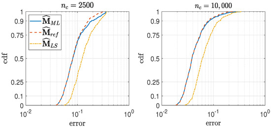
Figure 2. Empirical cdf of the errors of the 3 maximum likelihood estimators with 4 qubits.

• ${\widehat{\mathbf{M}}}_{ML}$ is very similar to its reference ${\widehat{\mathbf{M}}}_{ref}$ (especially with $n_c=10,000$). This means that the likelihood algorithm converges towards the global minimum (so 700 iterations is enough and ${\widehat{\mathbf{M}}}_{LS}$ is a good enough initial point).
• ${\widehat{\mathbf{M}}}_{LS}$ is worse than ${\widehat{\mathbf{M}}}_{ML}$. This means that the costly likelihood maximization is not made in vain.
• The errors with $n_c=10,000$ are roughly twice smaller than the errors with $n_c=2500$. So we are in the classic linear case where the error is proportional to the square root of the number of measurements. Additionally, the same graph with any $n_c>2500$ could be deduced from Figure 2.

6. Conclusions and Future Work

In this paper, we introduced two QPT methods that do not require the initial states to be set to predetermined values, but work with randomly selected initial states that are measured beforehand. The first method uses QST to estimate the input and output states, lifts the phase ambiguities and finds the unitary matrix which fits the estimated states the best. The second method finds the unitary matrix that is the most likely according to the statistical distribution of the measurements. The latter method is more precise but slower and uses the result of the first method as an initialization.

We intend to perform more extensive tests and compare our method to non-blind methods such as [7]. We also want to link this algorithm with that of [11] by considering fewer initial states and more time delays than in Figure 1.

References

- Ljung, L. System Identification: Theory for the User; PTR Prentice Hall: Upper Saddle River, NJ, USA, 1999; p. 540. [Google Scholar]
- Abed-Meraim, K.; Qiu, W.; Hua, Y. Blind system identification. Proc. IEEE 1997, 85, 1310–1322. [Google Scholar] [CrossRef]
- Nielsen, M.A.; Chuang, I.L. Prescription for experimental determination of the dynamics of a quantum black box. J. Mod. Opt. 2018, 44, 2455–2467. [Google Scholar]
- Nielsen, M.A.; Chuang, I.L. Quantum Computation and Quantum Information; Cambridge University Press: Cambridge, UK, 2000. [Google Scholar]
- Mohseni, M.; Rezakhani, A.T.; Lidar, D.A. Quantum-process tomography: Resource analysis of different strategies. Phys. Rev. A 2008, 77, 032322. [Google Scholar] [CrossRef]
- Shabani, A.; Kosut, R.; Mohseni, M.; Rabitz, H.; Broome, M.; Almeida, M.; Fedrizzi, A.; White, A. Efficient measurement of quantum dynamics via compressive sensing. Phys. Rev. Lett. 2011, 106, 100401. [Google Scholar] [CrossRef] [PubMed]
- Baldwin, C.H.; Kalev, A.; Deutsch, I.H. Quantum process tomography of unitary and near-unitary maps. Phys. Rev. A 2014, 90, 012110. [Google Scholar] [CrossRef]
- Deville, Y.; Deville, A. From blind quantum source separation to blind quantum process tomography. In Proceedings of the International Conference on Latent Variable Analysis and Signal Separation, Liberec, Czech Republic, 25–28 August 2015; Springer: Berlin/Heidelberg, Germany, 2015; pp. 184–192. [Google Scholar]
- Deville, Y.; Deville, A. The blind version of quantum process tomography: Operating with unknown input values. IFAC-PapersOnLine 2017, 50, 11731–11737. [Google Scholar] [CrossRef]
- Deville, Y.; Deville, A. Quantum process tomography with unknown single-preparation input states: Concepts and application to the qubit pair with internal exchange coupling. Phys. Rev. A 2020, 101, 042332. [Google Scholar] [CrossRef]
- Verdeil, F.; Deville, Y.; Deville, A. Two-Qubit Unitary Quantum Process Tomography by Multiple-Delay Output Measurements for One Unknown Input Pure State Value. In Proceedings of the 2021 IEEE Statistical Signal Processing Workshop (SSP), Rio de Janeiro, Brazil, 11–14 July 2021; IEEE: New York, NY, USA, 2021; pp. 161–165. [Google Scholar]
- Verdeil, F.; Deville, Y. Pure state tomography with parallel unentangled measurements. Phys. Rev. A, 2022; (to appear). [Google Scholar]
- Goyeneche, D.; Cañas, G.; Etcheverry, S.; Gómez, E.; Xavier, G.; Lima, G.; Delgado, A. Five Measurement Bases Determine Pure Quantum States on Any Dimension. Phys. Rev. Lett. 2015, 115, 090401. [Google Scholar] [CrossRef] [PubMed]
- Finkelstein, J. Pure-state informationally complete and “really” complete measurements. Phys. Rev. A 2004, 70, 052107. [Google Scholar] [CrossRef]
- Wahba, G. A Least Squares Estimate of Satellite Attitude. SIAM Rev. 1965, 7, 409. [Google Scholar] [CrossRef]
- Hradil, Z.; Řeháček, J.; Fiurášek, J.; Ježek, M. 3 Maximum-Likelihood Methods in Quantum Mechanics. In Quantum State Estimation; Springer: Berlin/Heidelberg, Germany, 2004; pp. 59–112. [Google Scholar]
- Broyden, C.G. The convergence of a class of double-rank minimization algorithms. IMA J. Appl. Math. 1970, 6, 76–90. [Google Scholar] [CrossRef]
Publisher’s Note: MDPI stays neutral with regard to jurisdictional claims in published maps and institutional affiliations. |
© 2022 by the authors. Licensee MDPI, Basel, Switzerland. This article is an open access article distributed under the terms and conditions of the Creative Commons Attribution (CC BY) license (https://creativecommons.org/licenses/by/4.0/).