Proceeding Paper

Information Geometry Control under the Laplace Assumption †

by
Adrian-Josue Guel-Cortez
* and
Eun-jin Kim
Centre for Fluid and Complex Systems, Coventry University, Coventry CV1 2TT, UK
*
Author to whom correspondence should be addressed.
Presented at the 41st International Workshop on Bayesian Inference and Maximum Entropy Methods in Science and Engineering, Paris, France, 18–22 July 2022.
Phys. Sci. Forum 2022, 5(1), 25; https://doi.org/10.3390/psf2022005025
Published: 12 December 2022

Abstract

:
By combining information science and differential geometry, information geometry provides a geometric method to measure the differences in the time evolution of the statistical states in a stochastic process. Specifically, the so-called information length (the time integral of the information rate) describes the total amount of statistical changes that a time-varying probability distribution takes through time. In this work, we outline how the application of information geometry may permit us to create energetically efficient and organised behaviour artificially. Specifically, we demonstrate how nonlinear stochastic systems can be analysed by utilising the Laplace assumption to speed up the numerical computation of the information rate of stochastic dynamics. Then, we explore a modern control engineering protocol to obtain the minimum statistical variability while analysing its effects on the closed-loop system’s stochastic thermodynamics.

1. Introduction

Stochastic systems are ubiquitous and include a large set of complex systems, such as the time evolution of molecular motors [1], the stock market [2], decision making [3], population dynamics [4] or engineering systems with parameter uncertainties [5]. The description of stochastic dynamics commonly involves the calculation of time-varying probability density functions (PDFs) governed by a Fokker–Planck equation and its corresponding stochastic differential equation [1]. Since a time-varying PDF describes all the possible trajectories the stochastic system can take in time, such a formalism has been advantageously applied in emergent fields as stochastic thermodynamics [6] or inference control [7].
As time-varying PDFs contain enormous dynamical information, defining a metric of the path’s length that a stochastic system takes through time can bring benefits when, for example, designing “efficient” systems (for instance, see [8]). In this regard, the field of information geometry has brought to light a true metric of the differences in the time evolution of the statistical states in a stochastic process [9,10]. Specifically, the concept of information length (IL) [11,12], given by the time integral of the stochastic dynamics information rate, describes the total amount of statistical changes that a time-varying probability distribution takes through time. The previous works showed that IL provides a link between stochastic processes, complexity and geometry [12]. Additionally, IL has been applied to the quantification of hysteresis in forward–backward processes [8,13], correlation and self-regulation among different players [13], phase transitions [14], and prediction of sudden events [15]. It is worth noting that in nonlinear stochastic systems, IL is generally difficult to obtain because the analytical/numerical solution of the Fokker–Planck equation and the execution of stochastic simulations are usually complicated and computationally costly. Hence, analytical simplifications are advantageous to ease IL’s calculation while increasing the possibility of applying IL to broader practical scenarios [16].
Even though the information rate may seem purely like a statistical quantity, its meaning can be understood in relation to the thermodynamics [11,12]. This result is of great advantage as we may use it to quantify the effects, for example, that a minimum statistical variability (constant information rate) control could have on the system’s energetic behaviour. Note that the idea of thermodynamic informed control systems is not something new. For instance, since the beginning of the 21st century, various works have proposed the consideration of entropy-informed control protocols to generate “intelligent/efficient” systems (for further details, see [17] and the references therein). Yet, describing the effects of an information geometry-informed control protocol over the system’s stochastic thermodynamics is to be carried out.
In this regard, we consider the application of the so-called Laplace assumption (Gaussian approximation of the system’s time-varying PDF) to the computation of IL and the information rate for a set of nonlinear stochastic differential equations. By using this assumption, we derive the values of the entropy rate, entropy production and entropy flow and their relation to the information rate. Then, we formulate an optimisation problem for the minimum information variability control and study the closed-loop stochastic dynamics and thermodynamics in a numerical example. Thus, creating a connection between information geometry, stochastic thermodynamics and control engineering (Figure 1).
To help readers, in the following, we summarise our notations. R is the set of real numbers; x R n represents a column vector x of real numbers of dimension n; A R n × n represents a real matrix of dimension n × n (bold-face letters are used to represent vectors and matrices); Tr ( A ) corresponds to the trace of the matrix A ; | A | , vec ( A ) , A and A 1 are the determinant, vectorisation, transpose and inverse of matrix A , respectively. The value I n denotes the identity matrix of order n. Newton’s notation is used for the partial derivative with respect to the variable t (i.e. y t = y ˙ ). Finally, the average of a random vector ζ is denoted by μ : = x , the angular brackets representing the average.

2. Model

Throughout this work, the following set of nonlinear Langevin equations is considered
x ˙ = f ( x , u ) + ξ .
Here, f : R n R n is a function taking as input a vector x R n and a bounded smooth time-dependent deterministic function u ( t ) R to output a vector f ( x ) R n with elements f i ( i = 1 , 2 , . . . n ); ξ R n is a Gaussian stochastic noise given by an n dimensional vector of δ -correlated Gaussian noises ξ i ( i = 1 , 2 , . . . n ), with the following statistical property
ξ i ( t ) = 0 , ξ i ( t ) ξ j ( t 1 ) = 2 D i j ( t ) δ ( t t 1 ) , D i j ( t ) = D j i ( t ) , i , j = 1 , , n .
The Fokker–Planck equation of (1) is
p ˙ = · J = · f p + · D p = i = 1 n x i ( f i p ) + i , j = 1 n x i D i j x j p ,
where J = [ f i p D i p , , f n p D n p ] .

2.1. The Laplace Assumption

The Laplace assumption allows us to describe the solution of (3) through a fixed multivariable Gaussian distribution given by [4]
p ( x ; t ) = 1 | 2 π Σ | e 1 2 Q ( x ; t ) ,
where Q ( x ; t ) = 1 2 x μ ( t ) Σ 1 ( t ) x μ ( t ) , and μ ( t ) R n and Σ ( t ) R n × n are the mean and covariance value of the random variable x . The value of the mean μ ( t ) and covariance matrix Σ ( t ) can be obtained from the following result.
Proposition 1
(The Laplace assumption). Under the Laplace assumption, the dynamics of the mean μ and covariance Σ at any time t of a nonlinear stochastic differential system (1) are governed by the following differential equations
μ ˙ = f 1 ( μ , u ) + 1 2 Tr Σ H f 1 , f 2 ( μ , u ) + 1 2 Tr Σ H f 2 , , f n ( μ , u ) + 1 2 Tr Σ H f n
Σ ˙ = J f Σ + Σ J f + D + D
where H f i is the Hessian matrix of the function f i ( x , u ) , and J f is the Jacobian of the function f ( x , u ) .
Proof. 
See Appendix A. □
Note that when f i ( x ; t ) in (1) is a linear function defined as
f i ( x ; t ) : = A i x ( t ) + B i u ( t ) = j = 1 n a i j x j ( t ) + j p b i j u j ( t ) ,
i.e., we consider a set of particles driven by a harmonic potential ( A i x ( t ) ) and a deterministic force ( B i u ( t ) , the value H f i = 0 , meaning that the mean value μ is not affected by the covariance matrix Σ .

Limits of the Laplace Assumption

Since the Laplace assumption does not always hold, we first check on its limitation by considering the following cubic stochastic differential equation
x ˙ ( t ) = γ x ( t ) 3 + u ( t ) + ξ ( t ) ,
where ξ = 0 , ξ ( t ) ξ ( t ) = 2 D δ ( t t ) and γ R + . Then, we denote q ( x , t ) that is based on the Laplace Assumption, which take the following Gaussian form
q ( x , t ) = 1 2 π Σ e 1 2 ( x μ ) 2 Σ ,
where μ and Σ are determined by the solution of
μ ˙ = γ μ 3 + u 3 γ μ Σ ,
Σ ˙ = 6 γ Σ μ 2 + 2 D .
To obtain the real system PDF p ˜ ( x , t ) of system (8), we use stochastic simulations and kernel density estimators (for further details see [18]). Now, to highlight the limits of the Gaussian approximation q ( x , t ) , we apply the Kullback divergence (KL) D K L or relative entropy between the estimated p ˜ and the Gaussian approximation q of the time-varying system (8) PDFs defined as
D K L ( p ˜ | | q ) = R p ( x ; t ) log p ( x ; t ) q ( x ; t ) d x .
Figure 2 shows the KL divergence trough time between p ˜ and q when changing the parameters γ and D in Equation (8). The result shows that a valid LA requires a small damping (slow behaviour) and a wider noise amplitude in comparison with the initial value of Σ .

3. Stochastic Thermodynamics

Stochastic thermodynamics uses stochastic calculus to draw a connection between the “micro/mesoscopic stochastic dynamics” and the “macroscopic thermodynamics” [1,6]. In physical terms, this means that stochastic thermodynamics describes the interaction of a micro/mesoscopic system with one or multiple reservoirs (for instance, the dynamics of a Brownian particle suspended in a fluid in thermodynamic equilibrium described by a Langevin/Fokker Planck equation).

3.1. Entropy Rate

Given a time-varying multivariable PDF p ( x ; t ) , we can calculate the entropy rate, a fundamental concept of stochastic thermodynamics, as follows [20]
S ˙ ( t ) = d d t S ( t ) = R n p ˙ ( x ; t ) ln p ( x ; t ) d x = Π Φ .
Proposition 2.
Under the Laplace assumption, the value of entropy rate S ˙ , entropy production Π and entropy flow Φ is given by
S ˙ = Tr Σ 1 D + Tr ( J f ) = 1 2 Tr Σ 1 Σ ˙ ,
Π = Tr Σ 1 D + Tr f ( μ , u ) D 1 f ( μ , u ) + Tr J f D 1 J f Σ + 2 Tr ( J f ) ,
Φ = Tr f ( μ , u ) D 1 f ( μ , u ) + Tr J f D 1 J f Σ + Tr ( J f ) .
Proof. 
See Appendix B. □

3.2. Example

To illustrate the application of Proposition 2, consider the following Langevin form of the Duffing equation
x ˙ ( t ) = v ( t ) + ξ 1 ( t ) v ˙ ( t ) = δ v ( t ) α x ( t ) β x ( t ) 3 + γ cos ( ω t ) + ξ 2 ( t ) ,
where x ( t ) is the displacement at time t, v ( t ) = x ˙ ( t ) is the first derivative of x with respect to time, i.e., velocity, ξ is a delta correlated noise, and the values δ , α , β , γ and ω are given constants.
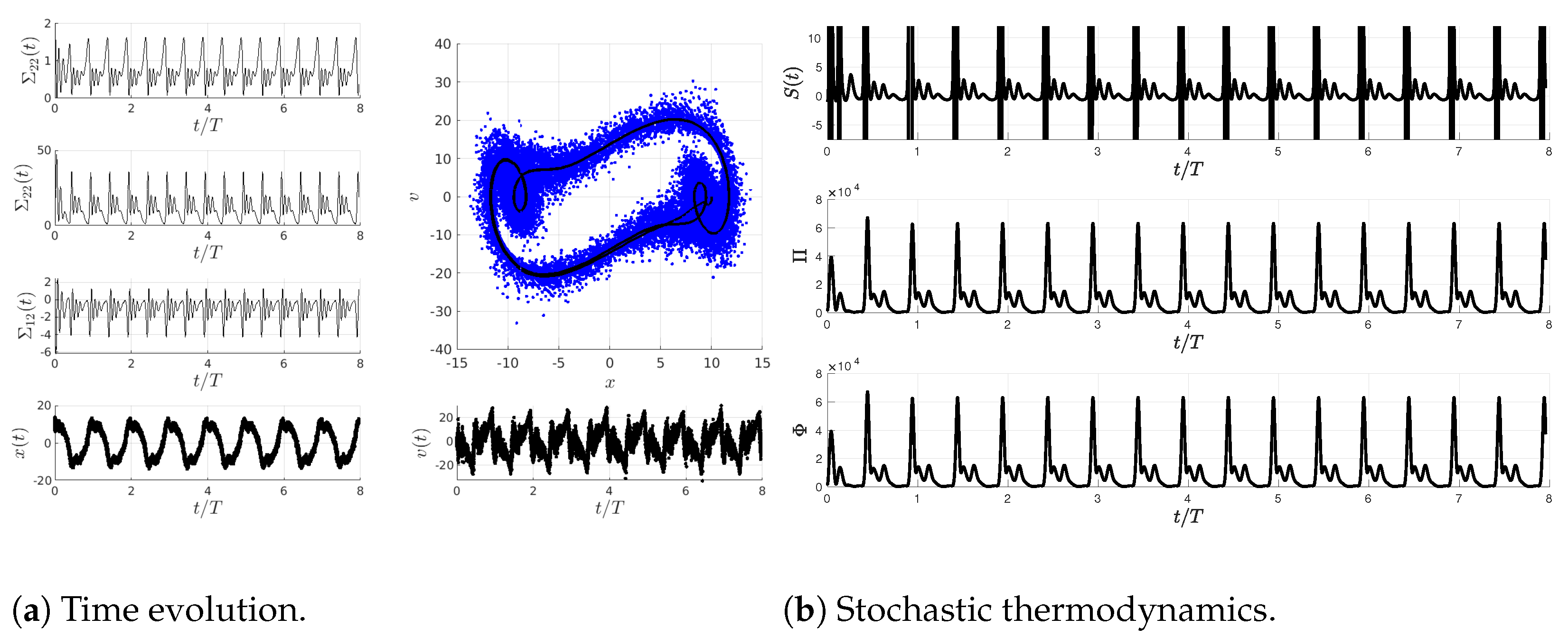
Figure 3 shows a simulation of (17) using the deterministic equations of the mean vector μ = [ x , v ] and covariance matrix Σ as described by Proposition 1. Specifically, Figure 3a includes the time evolution of the random variables x and v with its phase portrait, and the time evolution of Σ 11 , Σ 12 and Σ 22 . Figure 3b shows the time evolution of the system’s stochastic thermodynamics including the entropy rate S ˙ , the entropy production Π and the entropy flow Φ . In all subplots, time is scaled by the factor T = 2 π / ω .
More importantly, Figure 3 shows that via Propositions 1 and 2 it is possible to describe the thermodynamics of any nonlinear stochastic system at every instant of time. Hence, as will be discussed in Section 5, Propositions 1 and 2 allow us to perceive the effects of a control protocol on the closed-loop system thermodynamics.

4. Information Length and Information Rate

For a time-varying multivariable PDF p ( x ; t ) , we define its IL L as [15,16]
L ( t ) = 0 t R n p ( x ; τ ) τ ln p ( x ; τ ) 2 d x d τ = 0 t Γ ( τ ) d τ ,
where Γ is called the information rate. The value of Γ 2 can be understood as the Fisher information where the time is the control parameter [12]. Since Γ gives the rate of change of p ( x ; t ) , its time integral L quantifies the amount of statistical changes that the system goes through in time from the initial PDF p ( x ; 0 ) to a final PDF p ( x ; t ) [16].
Under the Laplace assumption, i.e., when p ( x ; t ) is a Gaussian PDF, the value of information rate Γ of the joint PDF takes the compact form [11,16]
Γ 2 = μ ˙ Σ 1 μ ˙ + 1 2 Tr ( Σ 1 Σ ˙ ) 2 ,
where the time derivatives of μ ˙ and Σ ˙ are given by Equations (5) and (6), respectively.

Relation with Stochastic Thermodynamics

Considering a fully decoupled nonlinear stochastic system and using the Laplace assumption, the value of the information rate Γ 2 is related to the entropy production Π and the entropy flow S ˙ as follows
Γ 2 = i = 1 n D i i Σ i i Π i + i = 1 n S ˙ i 2 + 1 2 i = 1 n H f i ( μ ˙ i + f i ( μ i , u ) ) ,
where Π i and S ˙ i are the entropy production and entropy rate from the marginal PDF p ( x i , t ) of x i . H f 1 = 2 x i 2 f i ( μ i , t ) . If f i describes a harmonic potential (7), then H f i = 0 and (20) lead to the expression
Γ 2 = i n D i i Σ i i Π i + i n S ˙ i 2 .
Note that Equation (21) gives us a case where a minimum information length L would produce both a minimum entropy production/rate and a minimum statistical variability behaviour.

5. Minimum Variability Control

To impose a minimum statistical variability when going from an initial to a desired state (for instance, see [21]), we propose the optimisation problem with the following cost function
c = arg min c ˜ J = 0 t f ( Γ ( t ) Γ ( 0 ) ) 2 + ( Y ( t ) Y d ) Q ( Y ( t ) Y d ) + c ˜ ( t ) R c ˜ ( t ) d t
where Y ( t ) : = [ μ ( t ) , vec ( Σ ( t ) ) ] , Y d : = [ μ d , vec ( Σ d ) ] , c ( t ) ˜ : = [ u ( t ) , vec ( D ( t ) ) ] , Q R n + n × n , and R R 1 + n × n . The solution c ( t ) corresponds to the control vector that allows us to obtain the minimum statistical variability. In Equation (22), the term ( Γ ( t ) Γ ( 0 ) ) 2 keeps the information variability constant. The term involving Q drives the system to reach a given PDF defined by Y d . The term containing R in the right-hand side of (22) regularises the control action c to avoid abrupt changes in the inputs. Note that the values of Σ , μ and Γ can be easily computed for any nonlinear stochastic process through Proposition (1) or the Laplace assumption. A control that comes after solving (22) would be called an information length quadratic regulator (IL-QR).

5.1. Model Predictive Control

A solution to the proposed optimisation problem (22) can be obtained by one of the most popular optimisation-based control techniques currently available—the so-called model-predictive-control (MPC) scheme [22]. Generally, MPC is an online optimisation algorithm for constrained control problems whose benefits have been recognized in applications to robotics [23], solar energy [24] or bioengineering [25]. Furthermore, MPC has the advantage of being easily implemented owing to packages such as CasADi [26] or the Hybrid Toolbox [27].
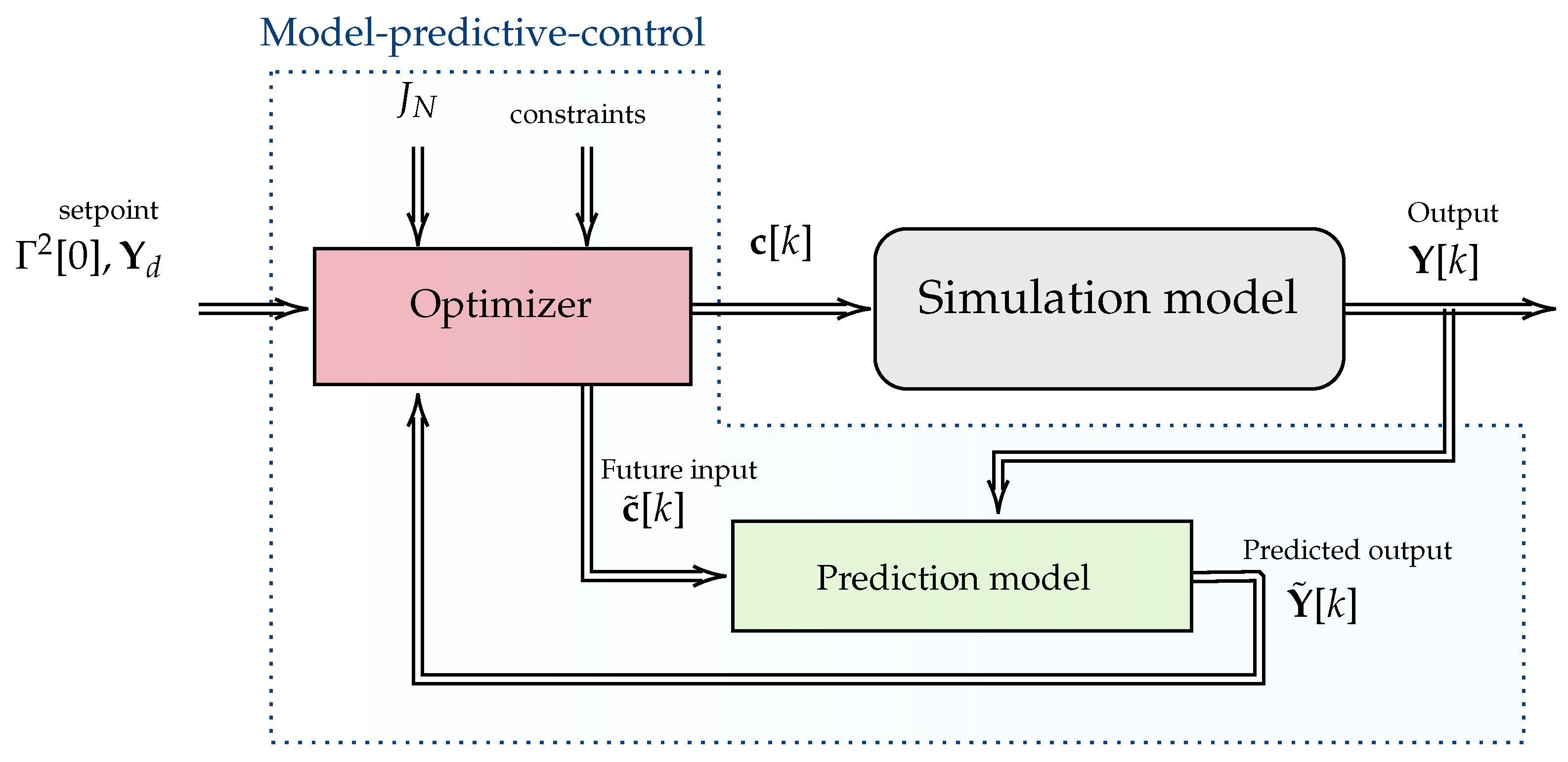
Figure 4 briefly details the working principle of the MPC’s optimiser in the form of a block diagram. The MPC method consists of utilising a prediction model to solve the optimisation problem in a finite horizon. Then, the optimal solution is applied to the system in real-time. Finally, the system’s output is fed back to the MPC algorithm to start the optimisation procedure again. In this work, we ease the prediction and simulation of the stochastic process by employing the Laplace assumption.

5.2. Example

We now present an example of the application of the MPC method to obtain the minimum variability behaviour of a stochastic system. Figure 5 shows the IL-QR applied to the cubic stochastic process given by Equation (8), where the control vector and the state vector are given by c = [ u , D ] and Y = [ μ , Σ ] , respectively. In the simulation, the initial state is Y ( 0 ) = [ 2 + 5 / 6 , 1 / ( 2 × 30 ) ] , while the desired state is Y d ( t ) = [ 2 + 1 / 30 , 1 / ( 2 × 3 ) ] . Additionally, we consider the parameters γ = 0.1 , T s = 1 × 10 3 , N = 5 , I L = 1 × 10 3 , R = 1 × 10 5 I 2 , Q 12 = Q 21 = 0 , Q 12 = 1 × 10 2 and Q 22 = 8 × 10 2 . Here, T s is the integration time step, and N is the number of future time steps considered in the prediction model. The value of Γ ( 0 ) is imposed via the initial conditions and Equation (19).
In Figure 5a, we show the time evolution of the mean μ , the inverse temperature β = 1 2 Σ , the input force u, the noise amplitude D, the information rate Γ 2 and the information length L . We also show the PDF time evolution of the simulation model computed via the Laplace approximation (q) or via stochastic simulations ( p ˜ ) and the corresponding K L -divergence (12) between them. In the subplot of μ and β , the legend LA and SS stand for the Laplace assumption and stochastic simulations, respectively. Interestingly, we can see from this that the Laplace approximation works fine when used as a prediction model in the MPC method. The controls have a chattering effect (oscillations having a finite frequency and amplitude) similar to the one encountered when implementing other control methods, such as the sliding mode control [28], when trying to keep the system in the desired state Y d .
Figure 5b demonstrates the effects of controls (22) on the closed-loop system stochastic thermodynamics. The results show that at the desired state Y d the value of S ˙ oscillates around zero with a small amplitude. This means Φ = Π holds at some instants of time when Y reaches Y d . In other words, all the energy is exchanged with the system’s environment when the control keeps Y on the nonequilibrium state Y d .

6. Conclusions

In this work, we developed a new control MPC method to derive the evolution of a system with a minimum information variability in systems governed by nonlinear stochastic differential equations. Specifically, we identified the limitations of the Laplace assumption and utilised it to reduce the computational cost of calculating the time-varying PDFs and to develop a prediction model in the MPC algorithm. We also derived the relations that permit us to analyse the controller effects on the close-loop system’s thermodynamics.
In future work, we aim to apply our results for maximising the free-energy (minimum entropy production) [12] and for the analysis of the closed-loop stochastic thermodynamics in higher-order systems.

Author Contributions

Conceptualization, A.-J.G.-C. and E.-j.K.; methodology, A.-J.G.-C.; software, A.-J.G.-C.; validation, A.-J.G.-C. and E.-j.K.; formal analysis, A.-J.G.-C.; investigation, A.-J.G.-C.; resources, A.-J.G.-C. and E.-j.K.; data curation, A.-J.G.-C.; writing—original draft preparation, A.-J.G.-C.; writing—review and editing, A.-J.G.-C. and E.-j.K.; visualization, A.-J.G.-C.; supervision, E.-j.K.; project administration, E.-j.K.; funding acquisition, E.-j.K. All authors have read and agreed to the published version of the manuscript.

Funding

This research received no external funding.

Institutional Review Board Statement

Not applicable.

Informed Consent Statement

Not applicable.

Data Availability Statement

Not applicable.

Conflicts of Interest

The authors declare no conflict of interest.

Appendix A. Proof of Proposition 1

To prove Proposition 1, we start by defining the first two moments of the ensemble density p ( x ) . This is given as follows
μ ˙ i = R n x i p ˙ ( x ; t ) d n x ,
Σ ˙ i j = R n x ¯ i x ¯ j p ˙ ( x ; t ) d n x .
Here, x ¯ i = x i μ i . Using (A1)–(A2) and (3), while avoiding the arguments for simplicity, we have
μ ˙ i = R n x i i = 1 n x i ( f i p ) + i , j = 1 n x i D i j x j p d n x , = R n x i x i ( f i p ) d n x + R n x i x i j = 1 n D i j x j p d n x , = R n f i p d n x = f i .
Σ ˙ i j = R n x ¯ i x ¯ j i = 1 n x i ( f i p ) + i , j = 1 n x i D i j x j p d n x , = R n x ¯ i x ¯ j x i ( f i p ) d n x R n x ¯ i x ¯ j x j ( f j p ) d n x + R n x ¯ i j = 1 n D i j x j p d n x + R n x ¯ j i = 1 n D j i x i p d n x , = x ¯ j f i + x ¯ i f j + D i j + D j i .
A closed-form solution to (A3)–(A4) can be obtained by exploiting the Laplace assumption; i.e., we recover the sufficient statistics (A1)–(A2) of system (1) through the first three terms of the nonlinear flow f i ( x , u ) Taylor expansion around the expected state μ . This is given as follows
f i ( x , u ) = f i ( μ , u ) + j = 1 n f i ( μ , u ) x j x ¯ j + 1 2 j , k = 1 n 2 f i ( μ , u ) x j x k x ¯ j x ¯ k +
Under Gaussian assumptions x ¯ i = 0 and x ¯ i x ¯ j = Σ i j and applying (A5) to (A3)–(A4), we have
μ ˙ = f i ( μ , u ) + j = 1 n f i ( μ , u ) x j x ¯ j + 1 2 j , k = 1 n 2 f i ( μ , u ) x j x k x ¯ j x ¯ k ,
= f i ( μ , u ) + 1 2 j , k = 1 n 2 f i ( μ , u ) x j x k Σ j k . Σ ˙ i j = x ¯ j + x ¯ i f i ( μ , u ) + k = 1 n f i ( μ , u ) x k x ¯ k + D i j + D j i ,
= k = 1 n f i ( μ , u ) x k Σ j k + k = 1 n f i ( μ , u ) x k Σ i k + D i j + D j i .
Equations (A6)–(A7) are the expansion of the equations shown in Proposition 1. This finishes the proof.

Appendix B. Proof of Proposition 2

By substituting (3) in (13), we obtain
d d t S ( t ) = R n i x i J i ( x ; t ) ln p ( x ; t ) d n x = R n i J i ( x ; t ) x i ln p ( x ; t ) d n x .
Now, after substituting the i t h term of J in (A8), we have
d d t S ( t ) = R n i J i ( x ; t ) f i ( x ; t ) D i i J i ( x ; t ) D i i p ( x ; t ) j i D i j x j p ( x ; t ) D i i p ( x ; t ) d n x .
From (A9), the entropy production rate of the system corresponds to the positive definite part
Π = i Π i = R n i J i ( x ; t ) 2 D i i p ( x ; t ) d n x ,
while the entropy flux (entropy from the system to the environment) is
Φ = R n i J i ( x ; t ) f i ( x ; t ) D i i j i D i j J i ( x ; t ) x j p ( x ; t ) D i i p ( x ; t ) d n x .
In this paper, we focus on the case when D i j = 0 if i j to simplify (A11) as
Φ = i Φ i = R n i J i ( x ; t ) f i ( x , t ) D i i d n x .
Notice that (A10)–(A11) require that D i i > 0 . If D i i = 0 , we have Π i = 0 and
Φ i = f i ( x , t ) x i .
We start by applying the definition of entropy (A10) production and entropy flux (A12), giving us
Π i = 1 D i i f i ( x , t ) 2 + D i i Q ( x ) x i 2 + 2 f i ( x , t ) x i ,
Φ i = 1 D i i f i ( x , t ) 2 + f i ( x , t ) x i .
Before continuing, it is useful to note that [29]
Q x k = 1 2 i x ¯ i Σ k i 1 + j x ¯ j Σ j k 1 = i x ¯ i Σ k i 1 = x ¯ Σ k 1
where x ¯ i = x i μ i , x ¯ : = x μ = [ x ¯ 1 , , x ¯ n ] and Σ k 1 is the k-th column of the inverse matrix Σ 1 of Σ . Therefore, [29]
D i i Q ( x ) x i 2 = D i i x ¯ Σ i 1 ( Σ i 1 ) x ¯ = D i i Tr ( Δ i Σ ) ,
and
f i ( x ) 2 D i i = 1 D i i f i ( μ , u ) + j = 1 n f i ( μ , u ) x j x ¯ j f i ( μ , u ) + k = 1 n f i ( μ , u ) x k x ¯ k = 1 D i i f i ( μ , u ) 2 + j , k = 1 n f i ( μ , u ) x j f i ( μ , u ) x k Σ j k = 1 D i i f i ( μ , u ) 2 + f i ( μ , u ) Σ f i ( μ , u ) ,
f i ( x , t ) x i = x i f i ( μ , u ) + j = 1 n f i ( μ , u ) x j x ¯ j + 1 2 j , k = 1 n 2 f i ( μ , u ) x j x k x ¯ j x ¯ k = f i ( μ , u ) x i .
Hence,
Π = i = 1 n Π i = Tr Σ 1 D + Tr D 1 f ( μ , u ) f ( μ , u ) + Tr J f D 1 J f Σ + 2 Tr ( J f )
Φ = i = 1 n Φ i = Tr D 1 f ( μ , u ) f ( μ , u ) + Tr J f D 1 J f Σ + Tr ( J f )
S ˙ = Tr Σ 1 D + Tr ( J f )

References

  1. Seifert, U. Stochastic thermodynamics, fluctuation theorems and molecular machines. Rep. Prog. Phys. 2012, 75, 126001. [Google Scholar] [CrossRef] [PubMed] [Green Version]
  2. Gontis, V.; Kononovicius, A. Consentaneous agent-based and stochastic model of the financial markets. PLoS ONE 2014, 9, e102201. [Google Scholar] [CrossRef] [PubMed] [Green Version]
  3. de Freitas, R.A.; Vogel, E.P.; Korzenowski, A.L.; Rocha, L.A.O. Stochastic model to aid decision making on investments in renewable energy generation: Portfolio diffusion and investor risk aversion. Renew. Energy 2020, 162, 1161–1176. [Google Scholar] [CrossRef]
  4. Marreiros, A.C.; Kiebel, S.J.; Daunizeau, J.; Harrison, L.M.; Friston, K.J. Population dynamics under the Laplace assumption. Neuroimage 2009, 44, 701–714. [Google Scholar] [CrossRef] [PubMed]
  5. Maybeck, P.S. Stochastic Models, Estimation, and Control; Academic Press: Cambridge, MA, USA, 1982. [Google Scholar]
  6. Peliti, L.; Pigolotti, S. Stochastic Thermodynamics: An Introduction; Princeton University Press: Princeton, NJ, USA, 2021. [Google Scholar]
  7. Baltieri, M.; Buckley, C.L. PID control as a process of active inference with linear generative models. Entropy 2019, 21, 257. [Google Scholar] [CrossRef] [PubMed] [Green Version]
  8. Kim, E.; Hollerbach, R. Geometric structure and information change in phase transitions. Phys. Rev. E 2017, 95, 062107. [Google Scholar] [CrossRef] [Green Version]
  9. Nielsen, F. An elementary introduction to information geometry. Entropy 2020, 22, 1100. [Google Scholar] [CrossRef]
  10. Amari, S.I. Information Geometry and Its Applications; Springer: Berlin/Heidelberg, Germany, 2016; Volume 194. [Google Scholar]
  11. Kim, E. Information geometry and nonequilibrium thermodynamic relations in the over-damped stochastic processes. J. Stat. Mech. Theory Exp. 2021, 2021, 093406. [Google Scholar] [CrossRef]
  12. Kim, E. Information Geometry, Fluctuations, Non-Equilibrium Thermodynamics, and Geodesics in Complex Systems. Entropy 2021, 23, 1393. [Google Scholar] [CrossRef]
  13. Hollerbach, R.; Kim, E.; Schmitz, L. Time-dependent probability density functions and information diagnostics in forward and backward processes in a stochastic prey–predator model of fusion plasmas. Phys. Plasmas 2020, 27, 102301. [Google Scholar] [CrossRef]
  14. Kim, E.; Heseltine, J.; Liu, H. Information length as a useful index to understand variability in the global circulation. Mathematics 2020, 8, 299. [Google Scholar] [CrossRef] [Green Version]
  15. Guel-Cortez, A.J.; Kim, E. Information Geometric Theory in the Prediction of Abrupt Changes in System Dynamics. Entropy 2021, 23, 694. [Google Scholar] [CrossRef] [PubMed]
  16. Guel-Cortez, A.J.; Kim, E. Information length analysis of linear autonomous stochastic processes. Entropy 2020, 22, 1265. [Google Scholar] [CrossRef] [PubMed]
  17. Saridis, G.N. Entropy in Control Engineering; World Scientific: Singapore, 2001; Volume 12. [Google Scholar]
  18. Fan, J.; Marron, J.S. Fast implementations of nonparametric curve estimators. J. Comput. Graph. Stat. 1994, 3, 35–56. [Google Scholar]
  19. Stochastic Simulation Versus Laplace Assumption in a Cubic System. Available online: https://github.com/AdrianGuel/StochasticProcesses/blob/main/CubicvsLA.ipynb (accessed on 6 June 2022).
  20. Tomé, T. Entropy production in nonequilibrium systems described by a Fokker-Planck equation. Braz. J. Phys. 2006, 36, 1285–1289. [Google Scholar] [CrossRef] [Green Version]
  21. Soto, F.; Wang, J.; Ahmed, R.; Demirci, U. Medical micro/nanorobots in precision medicine. Adv. Sci. 2020, 7, 2002203. [Google Scholar] [CrossRef] [PubMed]
  22. Lee, J.H. Model predictive control: Review of the three decades of development. Int. J. Control. Autom. Syst. 2011, 9, 415–424. [Google Scholar] [CrossRef]
  23. Mehrez, M.W.; Worthmann, K.; Cenerini, J.P.; Osman, M.; Melek, W.W.; Jeon, S. Model predictive control without terminal constraints or costs for holonomic mobile robots. Robot. Auton. Syst. 2020, 127, 103468. [Google Scholar] [CrossRef]
  24. Kristiansen, B.A.; Gravdahl, J.T.; Johansen, T.A. Energy optimal attitude control for a solar-powered spacecraft. Eur. J. Control 2021, 62, 192–197. [Google Scholar] [CrossRef]
  25. Salesch, T.; Gesenhues, J.; Habigt, M.; Mechelinck, M.; Hein, M.; Abel, D. Model based optimization of a novel ventricular assist device. at-Automatisierungstechnik 2021, 69, 619–631. [Google Scholar] [CrossRef]
  26. Andersson, J.A.E.; Gillis, J.; Horn, G.; Rawlings, J.B.; Diehl, M. CasADi—A software framework for nonlinear optimization and optimal control. Math. Program. Comput. 2019, 11, 1–36. [Google Scholar] [CrossRef]
  27. Bemporad, A. Hybrid Toolbox—User’s Guide. 2004. Available online: http://cse.lab.imtlucca.it/~bemporad/hybrid/toolbox (accessed on 1 June 2022).
  28. Utkin, V.; Lee, H. Chattering problem in sliding mode control systems. In Proceedings of the International Workshop on Variable Structure Systems, Alghero, Sardinia, 5–7 June 2006; pp. 346–350. [Google Scholar]
  29. Petersen, K.B.; Pedersen, M.S. The matrix cookbook. Tech. Univ. Den. 2008, 7, 510. [Google Scholar]
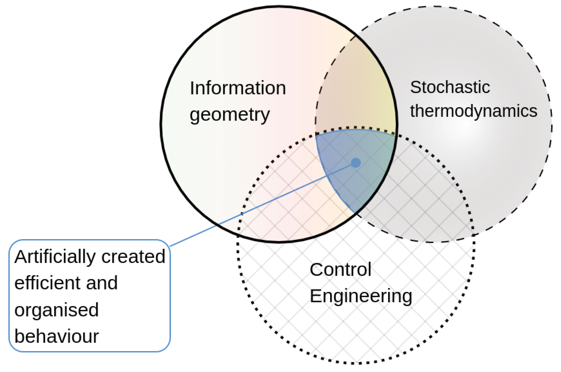
Figure 1. The combination of methods from information geometry, stochastic thermodynamics and control engineering may lead to the creation of energetically efficient and organised behaviour.
Psf 05 00025 g001
Figure 2. KL divergence between the value p ˜ ( x ; t ) and the value q ( x , y ) varying the values γ and D of Equation (8). When γ changes, D = 0.01 ; when D changes, γ = 0.01 . The initial condition is a Gaussian distribution defined by μ ( 0 ) = 5 and Σ ( 0 ) = 0.01 . See code at [19].
Psf 05 00025 g002
Figure 3. Simulation of dynamics and stochastic thermodynamics of the Duffing equation under the Laplace assumption.
Psf 05 00025 g003
Figure 4. Model predictive control block diagram.
Psf 05 00025 g004
Figure 5. IL-QR under LA applied to system (8) with Y ( 0 ) = [ 2 + 5 / 6 , 1 / ( 2 × 30 ) ] and Y d ( t ) = [ 2 + 1 / 30 , 1 / ( 2 × 3 ) ] . The control is applied in u ( t ) and D ( t ) . Moreover, γ = 0.1 , T s = 1 × 10 3 , N = 5 , I L = 1 × 10 3 , R = 1 × 10 5 I 2 , Q 12 = Q 21 = 0 , Q 12 = 1 × 10 2 and Q 22 = 8 × 10 2 .
Psf 05 00025 g005
Publisher’s Note: MDPI stays neutral with regard to jurisdictional claims in published maps and institutional affiliations.