Model-Based and Physics-Informed Deep Learning Neural Network Structures ^†

Abstract

Neural Networks (NNs) have been used in many areas with great success. When an NN’s structure (model) is given, during the training steps, the parameters of the model are determined using an appropriate criterion and an optimization algorithm (training). Then, the trained model can be used for the prediction or inference step (testing). As there are also many hyperparameters related to optimization criteria and optimization algorithms, a validation step is necessary before the NN’s final use. One of the great difficulties is the choice of NN structure. Even if there are many “on the shelf” networks, selecting or proposing a new appropriate network for a given data signal or image processing task, is still an open problem. In this work, we consider this problem using model-based signal and image processing and inverse problems methods. We classify the methods into five classes: (i) explicit analytical solutions, (ii) transform domain decomposition, (iii) operator decomposition, (iv) unfolding optimization algorithms, (v) physics-informed NN methods (PINNs). A few examples in each category are explained.

1. Introduction

Neural Networks (NNs), and in particular Deep Neural Networks (DNNs), have been used in many areas with great success, including in the following main areas: Computer Vision, speech recognition, and Artificial Intelligence (AI) with Large Language Models (LLMs).

Nowadays, there are a great number of DNN models which are freely accessible for different uses. However, when an NN’s structure (model) is selected, there is a choice between either a pre-trained NN ready for use in the special domain of interest or one that we want to train and use for our application. In this case, in general, we have to follow the following steps:

• Training step: For this, we need to access the training data in a data base. Then, we have to choose an appropriate criterion based on the category of the problem to be solved: Classification, Clustering, Regression, etc. The next step is to choose an appropriate optimization algorithm, some parameters, such as the learning rate, and finally, train the model. This means that the parameters of the model are obtained at the end of the convergence of the optimization algorithm.
• Model validation and hyperparameter tuning: As there are many hyperparameters (related to the optimization criteria and optimization algorithms), a validation step is necessary before the final use of the model. In this step, in general, we may use a subset of the training data or some other good-quality training data in which we can be confident, to tune the hyperparameters of the model and validate it.
• The last step before using the model is testing it and evaluating its performance on a testing data set. There are also a great number of testing and evaluation metrics, which have to be selected appropriately depending on the objectives of the considered problem.
• The final step is uploading the implemented model and using it. The amount of memory needed for this step has to be considered.

All these steps are very well studied, and many solutions have been proposed. One of the great difficulties is, in fact, in the first step: the choice of NN structure. Even if there are many “on the shelf” networks, selecting or proposing a new appropriate network for a given data, signal, or image processing task is still an open problem with the following key questions: Which structure should be chosen? How many layers are sufficient? Which kind of layer is most effective: dense ones or convolutional ones?

In this paper, we consider this problem using model-based signal and image processing and inverse problems methods. We classify the methods into five classes:

• Methods based on explicit analytical solutions;
• Methods based on transform domain processing;
• Methods based on the operator decomposition structure;
• Methods based on the unfolding of iterative optimization algorithms;
• Methods known as physics-informed NNs (PINNs).

A few examples from each category are explained.

The structure of the rest of this paper is as follows: As we focus on forward modeling and inverse problems methods, in Section 2, we present first two inverse problems that we will use later as the applications of the developed methods: infrared imaging (IR) and acoustical imaging. In Section 3, a short presentation of the Bayesian inference framework and its link with deterministic regularization methods are presented. From this point, the four previously mentioned categories of methods for selecting the structure of the NN are presented in detail in Section 4, Section 5, Section 6 and Section 7. Finally, applications of these methods in industry are briefly presented, and the conclusions of this work are given.

2. Inverse Problems Considered

2.1. Infrared Imaging

In many industrial application, infrared cameras are used to measure temperature remotely. The thermal radiation propagates from the source to the front of the camera, and is then transformed into a current measured by the CCDs of the infrared camera. If we represent the radiated source temperature distribution as $f(x,y)$, and the measured infrared energy distribution as $g(x,y)$, a very simplified forward model relating them can be given:

$$g(x,y)=\int \int h(x-x^{\prime },y-y^{\prime })\varphi (f(x^{\prime },y^{\prime }))d{x}^{\prime }d{y}^{\prime }=h(x,y)\ast \varphi (f(x,y)),$$

(1)

where * stands for 2D convolution. In this very simplified model, $h(x,y)$ is a convolution kernel function, also called the point spread function (PSF), approximating the propagation of the thermal diffusion, and $\varphi (.)$ is a nonlinear function which is given by

$$\varphi (f)={\varphi }_{\theta }(f)={\left[{\displaystyle \frac{e{f}^n+(1-e)T_u^n+(\exp \left[-kd\right]-1)T_a}{\exp \left[kd\right]}}\right]}^{1/n},$$

(2)

where $\theta =\{e,T_u,k,d,T_a\}$ is a set of parameters: e is the emissivity; $T_u$ is the background temperature; k is the attenuation coefficient, which can be a function of the humidity; d is the distance; and $T_a$ is the air temperature [1,2,3,4].

The convolution kernel can be obtained experimentally or assumed, for example, to be a Gaussian shaped with a known or unknown width parameter. Figure 1 shows the forward model.

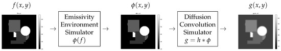
Figure 1. Infrared simplified forward model: The real temperature distribution as input $f(x,y)$, the nonlinear emissivity and environment perturbation function as $\varphi (f)$, the convolution operation to simulate the diffusion process, and finally the measured infrared camera output $g(x,y)$.

Figure 2 shows the corresponding inverse problem. The solution is either obtained by inversion or by a Neural Network.

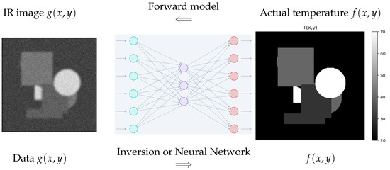
Figure 2. Infrared imaging: Forward model and inverse problem resolved either by mathematical inversion or by a Neural Network.

2.2. Acoustical Imaging

In acoustical imaging, a network of microphones receive signals emitted by sources with different delays:

$$g(x^{\prime },y^{\prime },t)=\int \mathrm{d}\omega \int \int f(x,y)\exp \left[-j\omega (t-\tau (x^{\prime }-x,y^{\prime }-y))\right]\mathrm{d}x\mathrm{d}y,$$

(3)

where $f(x,y)$ is the intensity of the source distribution at positions $(x,y)$, $g(x^{\prime },y^{\prime },t)$ is the received signal at positions $(x^{\prime },y^{\prime })$ of the microphones, $\omega$ is the frequency of the emitting source, and $\tau (x^{\prime }-x,y^{\prime }-y)$ is the the delay between the emitted source component at position $(x,y)$ and the position $(x^{\prime },y^{\prime })$ of the microphones, which is a function of the sound’s speed and the distance $d=\sqrt{{(x^{\prime }-x)}^2+{(y^{\prime }-y)}^2}$. See [5,6,7] for more details. Figure 3 shows the forward model.

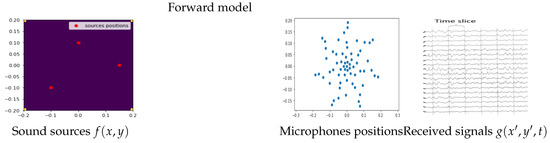
Figure 3. Forward model in acoustical imaging: each microphone receives the sum of the delayed source sounds.

In classical acoustical imaging, the inversion is made in two steps: Beamforming (BF) and Deconvolution. In BF, the received signals are delayed in opposite directions using the positions of the microphones, thus forming an image $b(x,y)$, which is shown to be related to the actual sound source distribution $f(x,y)$ via a convolution operation. Thus, the inverse problem is composed of two steps: Beamforming and Deconvolution. This last step can be down either in classical inversion or via a Neural Network [8]. Figure 4 shows these steps.

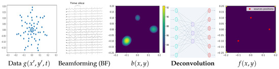
Figure 4. Acoustical imaging inverse problem via Beamforming (BF) and Deconvolution (Dec): In the first step, the received data are used to obtain an image $b(x,y)$ by BF, and then an inversion by Dec results in a good estimate of the sources.

3. Bayesian Inference for Inverse Problems

As the main aim of this paper is to explain the link between inverse problems and Neural Networks, and as the Bayesian inference approach is an appropriate one for defining solutions for them, in this section we very briefly summarize the Bayesian approach, specifically to inverse problems. Starting with the simple case of linear inverse problems $\mathit{g}=\mathit{H}\mathit{f}+\mathit{ϵ}$ and Gaussian prior models for the unknown image f and the observation noise $\mathit{ϵ}$, we summarize this approach in Figure 5:

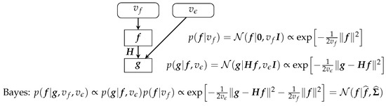
Figure 5. Basic Bayesian approach illustration for the case of Gaussian priors.

Then, we can easily obtain the following relations:

$$p(\mathit{f}|\mathit{g},v_f,v_{ϵ})=\mathcal{N}(\mathit{f}|\widehat{\mathit{f}},\widehat{\mathbf{\Sigma }}),\mathrm{with}\left\{\begin{array}{c}\widehat{\mathit{f}}={[{\mathit{H}}^{\prime }\mathit{H}+\lambda \mathit{I}]}^{-1}{\mathit{H}}^{\prime }\mathit{g}\hfill \\ \widehat{\mathbf{\Sigma }}=v_{ϵ}{[{\mathit{H}}^{\prime }\mathit{H}+\lambda \mathit{I}]}^{-1},\lambda ={\displaystyle \frac{v_{ϵ}}{v_f}}\hfill \end{array}\right..$$

(4)

In this particular Gaussian case, as the expected value and the mode are the same, the computation of $\widehat{\mathit{f}}$ can be done by an optimization, the Maximum A Posteriori (MAP) solution:

$$\widehat{\mathit{f}}=arg\underset{\mathit{f}}{max}\left\{p(\mathit{f}|\mathit{g},v_f,v_{ϵ})\right\}=arg\underset{\mathit{f}}{min}\left\{J(\mathit{f})\right\}\mathrm{where}J(\mathit{f})={\parallel \mathit{g}-\mathit{H}\mathit{f}\parallel }_2^2+\lambda {\parallel \mathit{f}\parallel }_2^2,\lambda ={\displaystyle \frac{v_{ϵ}}{v_f}}.$$

(5)

However, the computation of $\widehat{\mathbf{\Sigma }}$ is much more costly. There are many approximation methods such as MCMC sampling methods, Perturbation Optimization, Langevin sampling, and Variational Bayesian Approximation (VBA). The following figure summarizes the linear Gaussian case.

4. NN Structures Based on Analytical Solutions

4.1. Linear Analytical Solutions

As we could see in the previous section, the solution of the inverse problem, in the particular case of a linear forward model and Gaussian priors, is given by

$$\widehat{\mathit{f}}={(\mathit{H}{\mathit{H}}^t+\lambda \mathit{I})}^{-1}{\mathit{H}}^t\mathit{g}=\mathit{A}\mathit{g}=\mathit{B}{\mathit{H}}^t\mathit{g}={\mathit{H}}^t({\displaystyle \frac{1}{\lambda }}{\mathit{H}{\mathit{H}}^t+\mathit{I})}^{-1})\mathit{g}={\mathit{H}}^t\mathit{C}\mathit{g}.$$

(6)

These relations are shown schematically in Figure 6.

Figure 6. Three NN structures based on analytical solution expressions.

• ${\mathit{H}}^t$ can be implemented directly or by a Neural Network (NN)
• When H is a convolution operator, ${\mathit{H}}^t$ is also a convolution operator and can be implemented by a Convolutional Neural Network (CNN).
• $\mathit{B}={(\mathit{H}{\mathit{H}}^t+\lambda \mathit{I})}^{-1}$ and $\mathit{C}=({\displaystyle \frac{1}{\lambda }}{\mathit{H}{\mathit{H}}^t+\mathit{I})}^{-1})$ are, in general, dense NNs.
• When H is a convolution operator, B and C can also be approximated by convolution operators, and so by CNNs.

4.2. Feed-Forward and Residual NN Structure

Let us consider the case of denoising problem $\mathit{g}=\mathit{f}+\mathit{ϵ},$ where f is the original, ϵ is the noise, and g is the observed noisy image. Let us also to consider the case of a linear denoising method, obtained by a one-layer dense Feed-Forward network, $\widehat{\mathit{f}}=\mathit{A}(\mathit{g})$, as shown in Figure 7.

Figure 7. Feed-Forward NN structure.

If, in place of directly searching for the denoised solution, we first use an NN to obtain the noise and then obtain the denoised image by substraction $\widehat{\mathit{ϵ}}=\mathit{A}(\mathit{g})\to \widehat{\mathit{f}}=\mathit{g}-\widehat{\mathit{ϵ}}$, we obtain the Residual Network structure, shown in Figure 8.

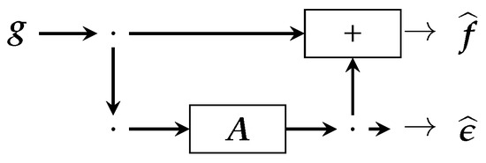
Figure 8. Residual structure NN.

5. NN Structures Based on Transformation and Decomposition

When the inverse operator A exists and is a linear operation, it can always be decomposed by three operations: Transformation T, transform domain operation O, and Inverse Transform ${\mathit{T}}^{-1}$ or Adjoint Transform ${\mathit{T}}^T$. This structure is shown in Figure 9.:

Figure 9. Transform domain NN structure.

Two such transformations are very important: Fourier Transform (FT) and Wavelet Transform (WT).

5.1. Fourier Transform-Based Networks

FT-Drop Out-IFFT can be presented as $\widehat{\mathit{f}}={\mathit{F}}^T\left[\mathbf{\Lambda }\mathit{F}\left[\mathit{g}\right]\right]$, which results in the FTNN shown in Figure 10.

Figure 10. Fourier Transform domain NN structure.

5.2. Wavelet Transform-Based Networks

Wavelet Transform–Drop Out–Inverse Wavelet Transform is defined as $\widehat{\mathit{f}}={\mathit{W}}^T\left[\mathbf{\Lambda }\mathit{W}\left[\mathit{g}\right]\right]$, which results in the WTNN shown in Figure 11.

Figure 11. Wavelet Transform domain NN structure.

We may note that, for image processing, in FT there is one channel and in WT there are four or more channels.

5.3. NN Structures Based on Operator Decomposition and Encoder–Decoder Structure

A more general operator decomposition can be

$$\text{Encoder–Decoder:}\hspace{1em}\hspace{1em}\mathit{A}(\mathit{g})={\mathit{A}}_{Dec}({\mathit{A}}_{Enc}(\mathit{g}))\hspace{1em}\hspace{1em}\mathit{g}\to \boxed{{\mathit{A}}_{Enc}}\to \boxed{{\mathit{A}}_{Dec}}\to \widehat{\mathit{f}}$$

Each part, the Encoder and Decoder, can also be decomposed through a series of partial operators

${\mathit{A}}_{Enc}(\mathit{g})$: N-Layer Network: ${\mathit{C}}_0={\mathit{E}}_0(\mathit{g})$, ${\mathit{C}}_1={\mathit{E}}_1({\mathit{C}}_0)$, ${\mathit{C}}_2={\mathit{E}}_2({\mathit{C}}_1)$, ${\mathit{C}}_{N-1}={\mathit{E}}_N({\mathit{C}}_N)$, ⋮, ${\mathit{A}}_{Dec}(\mathit{g})={\mathit{C}}_{N-1}$

${\mathit{A}}_{Dec}(\mathit{g})$: N-Layer Network: ${\overline{\mathit{C}}}_{N-2}={\mathit{D}}_{N-1}({\mathit{C}}_{N-1})$, ⋮, ${\overline{\mathit{C}}}_2={\mathit{D}}_3({\overline{\mathit{C}}}_3)$, ${\overline{\mathit{C}}}_1={\mathit{D}}_2({\overline{\mathit{C}}}_2)$, ${\overline{\mathit{C}}}_0={\mathit{D}}_1({\overline{\mathit{C}}}_1)$, $\mathit{A}(g)={\overline{\mathit{C}}}_0=\widehat{\mathit{f}}$

which results in the Encoder–Decoder NN shown in Figure 12.

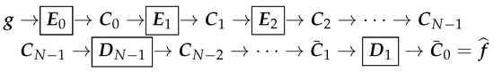
Figure 12. Encoder–Decoder structure based on operator decomposition.

6. DNN Structures Obtained by Unfolding Optimization Algorithms

Considering linear inverse problems such as $\mathit{g}=\mathit{H}\mathit{f}+\mathit{ϵ}$ within the Bayesian framework, with Gaussian errors, double exponential priors, and MAP estimation, or equivalently the ${\ell }_1$ regularization framework, the inversion becomes the optimization of the following criterion:

$$J(\mathit{f})={\parallel \mathit{g}-\mathit{H}\mathit{f}\parallel }_2^2+\lambda {\parallel \mathit{f}\parallel }_1$$

(7)

which can be obtained via an iterative optimization algorithm, such as ISTA:

$${\mathit{f}}^{(k+1)}=Pro{x}_{{\ell }_1}\left({\mathit{f}}^{(k)},\lambda \right)\stackrel{▵}{=}{\mathcal{S}}_{\lambda /\alpha }\left(\alpha {\mathit{H}}^t\mathit{g}+(\mathit{I}-\alpha {\mathit{H}}^t\mathit{H}){\mathit{f}}^{(k)}\right)$$

where ${\mathcal{S}}_{\theta }$ is a soft thresholding (ST) operator and $\alpha \le eig({\mathit{H}}^t\mathit{H})$ is the Lipschitz constant of the normal operator. Then, $(\mathit{I}-\alpha {\mathit{H}}^t\mathit{H}){\mathit{f}}^{(k)}$ can be considered as a filtering operator, $\alpha {\mathit{H}}^t\mathit{g}$ as a bias term, and ${\mathcal{S}}_{\theta }$ as a pointwise nonlinear operator. Thus, we obtain the unfolded structure shown in Figure 13.

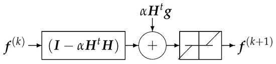
Figure 13. One iteration of an ${\ell }_1$ regularization optimization algorithm.

Now, if we consider a finite number of iterations, we can create a Deep Learning Network structure, shown in Figure 14.

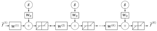
Figure 14. DLL structure based on a few iterations of the regularization optimization algorithm.

In Figure 14, if we choose ${\mathit{W}}_0=\alpha \mathit{H}$ and ${\mathit{W}}^{(k)}=\mathit{W}=(\mathit{I}-\alpha {\mathit{H}}^t\mathit{H}),k=1,\cdots ,K$, we obtain a more reasonable NN which can be more robust than the more general case ${\mathit{W}}^{(k)}=(\mathit{I}-{\alpha }^{(k)}{\mathit{H}}^t\mathit{H})$, where the parameters of each layer are different.

7. Physics-Informed Neural Networks (PINNs)

The main ideas behind PINNs are as follows:

• NNs are universal function approximators. Therefore an NN, provided that it is deep enough, can approximate any function, and also the solution for the differential equations.
• Computing the derivatives of an NN’s output with respect to any of its inputs (and the model parameters during backpropagation), using Automatic Differentiation (AD), is easy and cheap. This is actually what makes NNs so efficient and successful.
• Usually NNs are trained to fit the data, but do not care where those data come from. This is where physics-informed NNs come into play.
• Physics-based or physics-informed NNs: If, in addition to fitting the data, the NNs also fits the equations that govern that system and produce those data, their predictions will be much more precise and will generalize much better.

In the following section, we consider two cases: (i) a case where the forward model is explicitly given, alongside an operator H; (ii) a case where the forward model is given either by an ODE or PDE.

When the forward operator H is known, we can use it to propose the following structure and to define a criterion to use for optimizing the parameters of the NN. The main references on PINNs are [9,10,11,12].

7.1. PINN When an Explicit Forward Model Is Available

When an explicit forward model H is available, we can use it at the output of the NN, as shown in Figure 15.

Figure 15. A PINN when an explicit forward model H is available.

Here, the NN is used as a proxy or surrogate inversion method, in which parameter w is obtained by the optimization of the loss function $J(\mathit{g},\widehat{\mathit{g}})$. If, for an experiment, we have a set of data, we can use it to define a loss function with two parts, as shown in Figure 16.

Figure 16. A PINN when an explicit forward model H is available.

This can also be interpreted in a Bayesian way:

$$\begin{array}{cc}\hfill p(\mathit{g}|\mathit{f},{\sigma }_{ϵ}^2)& =\mathcal{N}(\mathit{g}|\mathit{H}\mathit{f},{\mathbf{\Sigma }}_{\mathit{ϵ}}),\mathrm{with}{\mathbf{\Sigma }}_{\mathit{ϵ}}={\sigma }_{ϵ}^2\mathit{I}\hfill \end{array}$$

(8)

$$\begin{array}{cc}\hfill p(\mathit{f}|{\sigma }_{ϵ}^2)& =\mathcal{N}(\mathit{f}|\overline{\mathit{f}},{\sigma }_f^2\mathit{I}),\mathrm{with}{\mathbf{\Sigma }}_f={\sigma }_f^2\mathit{I}\hfill \end{array}$$

(9)

One last extension is to define the loss function as

$$J(\mathit{g},\widehat{\mathit{g}})=\mathrm{Tr}\left[{\mathbf{\Sigma }}_{\mathit{ϵ}}\right]+\mathrm{Tr}\left[{\mathbf{\Sigma }}_f\right]\mathrm{with}{\mathbf{\Sigma }}_{\mathit{ϵ}}=\sum _i[{\mathit{g}}_i-{\widehat{\mathit{g}}}_i]{[{\mathit{g}}_i-{\widehat{\mathit{g}}}_i]}^t,\mathrm{and}{\mathbf{\Sigma }}_f=\sum _i[{\mathit{f}}_i-\overline{\mathit{f}}]{[{\mathit{f}}_i-\overline{\mathit{f}}]}^t.$$

(10)

In this way, at the end of training, we also have a good estimate of the covariances ${\mathbf{\Sigma }}_{\mathit{ϵ}}$ and ${\mathbf{\Sigma }}_f$, which can, eventually, be used as uncertainty priors for a new test input ${\mathit{g}}_j$.

7.2. A PINN When the Forward Model Is Described by an ODE or a PDE

PINNs for inverse problems modeled by an ODE or PDE were conceptually proposed by Raissi et al. back in 2017 [9]. Since then, there have been many works on the subject. See, for example [13,14,15,16] and [17,18].

The main idea consists in creating a hybrid model where both the observational data and the known physical knowledge are present in model training.

Inverse problems in ODEs or PDEs can be categorized into three increasingly difficult cases. To illustrate this, let us to consider a simple dynamical system:

• Unknown parameters model: As a simple dynamical system, consider

  $${\displaystyle \frac{\partial u}{\partial t}}=au+b,$$

  where the problem becomes estimating the parameters $\mathit{\theta }=(a,b)$.
• Unknown right side function:

  $${\displaystyle \frac{\partial u}{\partial t}}=f(t,u).$$
• Unknown parameters as well as the unknown function $f(t,u)$:

  $${\displaystyle \frac{\partial u}{\partial t}}=au+b+f(t,u)$$

The difference between a classical NN and physics-informed NN for a dynamical system, such as ${\displaystyle \frac{\partial u}{\partial t}}=f(t,u)$, can be illustrated as follows.

• Classical NN: The criterion to optimize is just a function of the output error, shown in Figure 17.
  

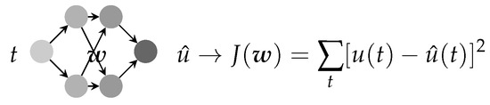  Figure 17. Classical NN: The criterion to optimize to obtain the NN parameter w is just a function of the output error.

• PINN: The criterion to optimize is a function of the output error and the forward error, shown in Figure 18.
  

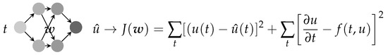  Figure 18. PINN: The criterion to optimize to obtain the NN parameter w is a function of the output error and the physics-based forward model error.

• Parametric PINN: When a parameter $\theta$ of the PDE is also unknown, we may also estimate it at the same time as the parameter w of the NN, as shown in Figure 19.
  

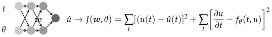  Figure 19. Parametric PINN: The unknown parameter $\theta$ of the PDE model can be optimized at the same time as the NN parameter w.

• Nonparametric PINN inverse problem: When the right-hand side of the ODE is an unknown function to be estimated too, we may consider a separate NN for it, as shown in Figure 20.
  

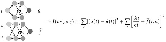  Figure 20. Nonparametric PINN: The unknown function f of the PDE model can also be approximated via a second NN, and the parameters ${\mathit{w}}_1$ and ${\mathit{w}}_2$ are optimized simultaneously.

• PINN for forward models described by PDE: For a more complex dynamical system with a PDE model, such as ${\displaystyle \frac{\partial u(x,t)}{\partial t}}+{\displaystyle \frac{\partial u(x,t)}{\partial x}}=u(x,t)$, the criterion must also account for the initial conditions (ICs), $\left[u(x,0)-\widehat{u}(x,0)\right]$, as well as the boundary conditions (BCs), $\left[u(0,t)+\widehat{u}(0,t)\right]$:

  $$\begin{array}{ccc}\hfill J(\mathit{w})& =& \sum _{x,t}{[u(x,t)-\widehat{u}(x,t)]}^2+\sum _{x,t}{\left[{\displaystyle \frac{\partial u(x,t)}{\partial t}}+{\displaystyle \frac{\partial u(x,t)}{\partial x}}-u(x,t)\right]}^2\hfill \\ & & +\sum _x{\left[u(x,0)-\widehat{u}(x,0)\right]}^2+\sum _t{\left[u(0,t)+\widehat{u}(0,t)\right]}^2\hfill \end{array}$$

Figure 21 shows the scheme of this case.

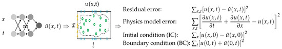
Figure 21. A PINN for forward models described by a PDE. Here, we have also account for the ICs and BCs.

8. Applications

We used these methods to develop innovative diagnostic and preventive maintenance systems for industrial systems (fans, blowers, turbines, wind turbines, etc.) using vibration, acoustics, infrared, and visible images. The main classical and NN methods we used are as follows:

• Vibration analysis using Fourier and Wavelet analysis;
• Acoustics: Sound source localization and estimation using acoustical imaging;
• Infrared imaging to monitor the temperature distribution;
• Visible images to monitor the system and its environment.

Figure 22 shows some of the experimental measurement systems we used.

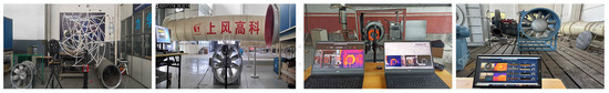
Figure 22. Experimental measurement systems we use for vibration, acoustics, infrared and visual images to develop innovative diagnostics and preventive maintenance.

An Example of Infrared Image Processing

Infrared images give a view of the temperature distribution, but they are low-resolution and very noisy. There is a need for their denoising, Deconvolution, super-resolution, segmentation, and real temperature reconstruction, as shown in Figure 23.

Figure 23. Infrared imaging: Denoising, Deconvolution, segmentation, and real temperature reconstruction.

Some preliminary results using Deep Learning methods in simulated and real situations are given in Figure 24.

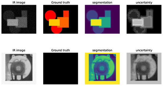
Figure 24. One typical example of Bayesian Deep Learning method results obtained for infrared image segmentation. (First row): Simulation results where we have a ground truth. (Second row): A real image where we do not have the ground truth.

9. Conclusions

The main conclusions of this work are as follows:

• Deep Neural Networks (DNNs) have been extensively used in Computer Vision and many other areas. There are, nowadays, a great number of NN structures, both “on the shelf” and user-selected, to try and use. If they work, they can be kept; if not, another can be selected, and so on!
• In particular, in inverse problems of Computer Vision, there is a need to guide the selection of an explainable structure, and so, explainable ML and AI are chosen.
• In this work, a few directions have been proposed. These methods are classified as model-based, physics-based, and physics-informed NNs (PINNs). Model-based and physics-based NNs have become a necessity for developing robust methods across all Computer Vision and imaging systems.
• PINNs were originally developed for inverse problems described by Ordinary or Partial Differential Equations (ODEs/PDEs). The main idea in all these problems is to appropriately choose NNs and use them as “Explainable” AI in industrial applications.

References

- Udayakumar, R.; Paulraj, C.; Kumar, S. Infrared thermography for condition monitoring–A review. Infrared Phys. Technol. 2013, 60, 35–55. [Google Scholar]
- Bhowmik, S.; Jha, M. Advances in infrared thermography for detection and characterization of defects in materials. Infrared Phys. Technol. 2012, 55, 363–371. [Google Scholar]
- Klein, T.; Maldague, X. Advanced thermography techniques for material inspection and characterization. J. Appl. Remote Sens. 2016, 10, 033508. [Google Scholar]
- Wang, L.; Zhao, P.; Ning, C.; Yu, L.; Mohammad-Djafari, A. A hierarchical Bayesian fusion method of infrared and visible images for temperature monitoring of high-speed direct-drive blower. IEEE Sens. J. 2022, 22, 18815–18830. [Google Scholar] [CrossRef]
- Chu, N.; Zhao, H.; Yu, L.; Huang, Q.; Ning, Y. Fast and High-Resolution Acoustic Beamforming: A Convolution Accelerated Deconvolution Implementation. IEEE Trans. Instrum. Meas. 2020, 70, 6502415. [Google Scholar] [CrossRef]
- Chen, F.; Xiao, Y.; Yu, L.; Chen, L.; Zhang, C. Extending FISTA to FISTA-Net: Adaptive reflection parameters fitting for the deconvolution-based sound source localization in the reverberation environment. Mech. Syst. Signal Process. 2024, 210, 111130. [Google Scholar] [CrossRef]
- Luo, X.; Yu, L.; Li, M.; Wang, R.; Yu, H. Complex approximate message passing equivalent source method for sparse acoustic source reconstruction. Mech. Syst. Signal Process. 2024, 217, 111476. [Google Scholar] [CrossRef]
- Nelson, C. Machine learning in acoustic imaging for industrial applications. J. Acoust. Mach. Learn. 2021, 5, 120–140. [Google Scholar]
- Raissi, M.; Perdikaris, P.; Karniadakis, G.E. Physics-informed neural networks: A deep learning framework for solving forward and inverse problems involving nonlinear partial differential equations. J. Comput. Phys. 2019, 378, 686–707. [Google Scholar] [CrossRef]
- Lu, L.; Meng, X.; Mao, Z.; Karniadakis, G.E. DeepXDE: A deep learning library for solving differential equations. SIAM Rev. 2021, 63, 208–228. [Google Scholar] [CrossRef]
- Karniadakis, G.E.; Kevrekidis, I.G.; Lu, L.; Perdikaris, P.; Wang, S.; Yang, L. Physics-informed machine learning. Nat. Rev. Phys. 2021, 3, 422–440. [Google Scholar] [CrossRef]
- Chen, W.; Cheng, X.; Habib, E.; Hu, Y.; Ren, G. Physics-informed neural networks for inverse problems in nano-optics and metamaterials. Opt. Express 2020, 28, 39705–39724. [Google Scholar] [CrossRef] [PubMed]
- Yang, L.; Meng, X.; Karniadakis, G.E. B-PINNs: Bayesian physics-informed neural networks for forward and inverse PDE problems with noisy data. J. Comput. Phys. 2021, 425, 109913. [Google Scholar] [CrossRef]
- Zhu, Y.; Zabaras, N.; Koutsourelakis, P.S.; Perdikaris, P. Physics-constrained deep learning for high-dimensional surrogate modeling and uncertainty quantification without labeled data. J. Comput. Phys. 2019, 394, 56–81. [Google Scholar] [CrossRef]
- Yang, Y.; Perdikaris, P. Adversarial uncertainty quantification in physics-informed neural networks. J. Comput. Phys. 2019, 394, 136–152. [Google Scholar] [CrossRef]
- Geneva, N.; Zabaras, N. Modeling the dynamics of PDE systems with physics-constrained deep auto-regressive networks. J. Comput. Phys. 2020, 403, 109056. [Google Scholar] [CrossRef]
- Gao, H.; Sun, L.; Wang, J.X. PhyGeoNet: Physics-informed geometry-adaptive convolutional neural networks for solving parameterized steady-state PDEs on irregular domain. J. Comput. Phys. 2021, 428, 110079. [Google Scholar] [CrossRef]
- Cai, S.; Wang, Z.; Wang, S.; Perdikaris, P.; Karniadakis, G.E. Physics-informed neural networks for heat transfer problems. J. Heat Transf. 2021, 143, 060801. [Google Scholar] [CrossRef]
Disclaimer/Publisher’s Note: The statements, opinions and data contained in all publications are solely those of the individual author(s) and contributor(s) and not of MDPI and/or the editor(s). MDPI and/or the editor(s) disclaim responsibility for any injury to people or property resulting from any ideas, methods, instructions or products referred to in the content. |
© 2025 by the authors. Licensee MDPI, Basel, Switzerland. This article is an open access article distributed under the terms and conditions of the Creative Commons Attribution (CC BY) license (https://creativecommons.org/licenses/by/4.0/).