A Straightforward Approach to Drawing Temperature-Dependent I–V Curves of Solar Cell Models

Abstract

Equivalent circuit models of solar cells are important for understanding the behavior of photovoltaic systems under different weather conditions. They provide an equation $F(V,I)=0$ that expresses the correspondence between voltage V and current I a cell can deliver. The performance of a cell, and, therefore, the parameters of equation F, depend on the cell’s temperature and on the incoming light’s energy and angle. One would like to simulate and visualize these dependencies in real time. Given a fixed set of parameters, no elementary solution $s\left(V\right)=I$ of Equation $F(V,I)=0$ is known. Hence, circuit simulation systems employ numerical methods to solve this equation and to approximate the circuit’s I–V curve, $C_{IV}$. In this note, we propose a simpler approach. Instead of expressing I as a function of V, we represent both as elementary functions $V\left(u\right)$ and $I\left(u\right)$ of a real parameter u. In this way, the I–V curve $C_{IV}$ is obtained as the image of the mapping $m\left(u\right)=\left(V\right(u),I(u\left)\right)$ from a u-interval to the $VI$-plane. Our approach offers both a precise mathematical description of $C_{IV}$ and an easy way to draw it. This allows us to study the influence of environmental changes on $C_{IV}$ by smooth animations, and yet with rather simple means. In this paper, we consider temperature dependence as an example; changes in irradiance or angle could be incorporated as well. Using formulae suggested in the literature that describe how the parameters in equation $F(V,I)=0$ depend on temperature, it takes only a few lines of code to generate an interactive worksheet that shows how $C_{IV}$, the location of the maximum power point MPP and the maximum power change as the circuit’s temperature, is altered on a slider. Such a worksheet and its location will be presented in this paper.

1. Introduction

Solar energy is of great importance to help us reduce, and finally eliminate, the use of fossil energy. As an increasing number of photovoltaic systems are appearing in public and in private installations, knowledge of their basic properties should be made easily accessible. On this note, we attempt to take a step in this direction. Before we get started, let us look at some background information first.

Both voltage V and current I generated by a photovoltaic cell depend on the load L it has to feed. In order to compute the maximum power $V·I$ the cell can deliver to suitable L, one needs to know the mutual dependency of V and I; that is, the I–V curve $C_{IV}$. To this end, different models of solar cells have been suggested.

Figure 1 shows the widely used single-diode model. Here, current I delivered to load L is given by

$$\begin{array}{ccc}\hfill I& =& I_{ph}-I_D-I_{sh}\hfill \end{array}$$

(1)

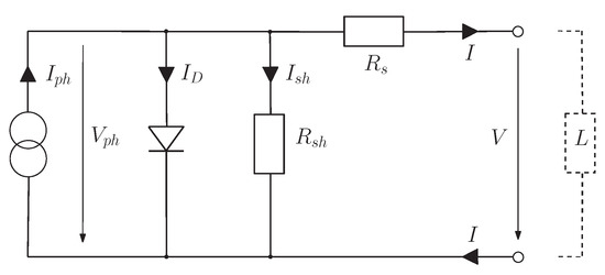
Figure 1. The single-diode model of a solar cell. $I_{ph}$ denotes the photogenetic current provided by the solar generator. One part of it, $I_D$, passes through the diode in a forward direction. Another part, $I_{sh}$, runs through shunt resistor $R_{sh}$; it models losses via leakage in the cell. The remaining current I passes through series resistor $R_s$, which represents losses caused by imperfect contacts. The values of I, voltage V and generator voltage $V_{ph}$ depend on the load L at the cell’s terminals.

A photogenetic current $I_{ph}$ is supposed to be provided by the solar generator. Both diode current $I_D$ and the current $I_{sh}$ through shunt resistor $R_{sh}$ depend on the voltage $V_{ph}$ at the generator, which is related to V by

$$\begin{array}{ccc}\hfill V_{ph}& =& V+I·R_s,\hfill \end{array}$$

(2)

taking the voltage drop at resistor $R_s$ into account. Using the Shockley diode equation to obtain $I_D$, Equation (1) implies the well-known formula

$$\begin{array}{ccc}\hfill I& =& I_{ph}-I_0·\left(exp\left(\frac{V+I·R_s}{n·V_T}\right)-1\right)-\frac{V+I·R_s}{R_{sh}}.\hfill \end{array}$$

(3)

Here, $I_0$ denotes the reverse saturation current of the diode, n equals the diode’s ideality factor, and $V_T$ stands for the thermal voltage.

Even when the values of $V_T,I_{ph}$, $I_0$, n, $R_s$ and $R_{sh}$ are known, the challenge is in expressing I as a function of V, or vice versa. To this end, one can rewrite (3) as equation

$$\begin{array}{ccc}\hfill 0=F(V,I)& =& I_{ph}-I_0·\left(exp\left(\frac{V+I·R_s}{n·V_T}\right)-1\right)-\frac{V+I·R_s}{R_{sh}}-I.\hfill \end{array}$$

(4)

The implicit function theorem [1] implies that there exist local solutions $I=s\left(V\right)$ satisfying $F(V,s(V\left)\right)=0$ in a neighborhood of each value of V, but an explicit expression for $s\left(V\right)$ by elementary functions (functions such as polynomials, roots, exp and ln, trigonometric functions and their inverses, and finite combinations of these are usually called elementary or of closed form) is not known. Thus, one has to resort to numerical methods.

In [2], it has been shown how to use Newton’s method to approximate, for a given voltage V, the associated current I, satisfying $F(V,I)=0$. The Newton method is a universal iterative algorithm for finding zeroes of smooth real-valued functions. For a sequence of V-values $V_j$, it can be used to approximate the associated values $I_j$ satisfying $F(V_j,I_j)=0$, with an accuracy depending on the number of iterations. Processing the values $V_j$ one by one leads to a sequence of points $(V_j,I_j)$ arbitrarily close to $C_{IV}$, but it does not provide us with a global solution $I=s\left(V\right)$ of equation $F(V,I)=0$ or, vice versa, a solution $V=r\left(I\right)$.

Then, in [3], such a solution $r\left(I\right)$ for V has been given in terms of the Lambert W-function,

$$\begin{array}{ccc}\hfill W\left(z\right)·exp\left(W\right(z\left)\right)& =& z.\hfill \end{array}$$

(5)

More precisely, the authors succeeded in separating the two variables V and I in (3) by providing an equation of type

$$\begin{array}{c}\hfill V=r\left(I\right)=a(I,W(b\left(I\right)\left)\right)\end{array}$$

(6)

with elementary functions a and b that involve the parameters of $F(V,I)$ but neither V nor I. Lambert function W itself is known to be not elementary, so that, again, it takes the Newton method or some other iterative algorithm to approximate it. However, because the W function occurs so frequently, efficient implementations of $W\left(z\right)$ are available in advanced math systems that can be used in commercial circuit simulators. They allow $C_{IV}$ curves to be drawn by a plot command that triggers numerous computations of W in the background.

The purpose of this paper is twofold. As a theoretical contribution, we present, in Section 3.1, an exact description of I–V curves by elementary functions. Instead of writing I as a function of V, we express both as functions $V\left(u\right)$ and $I\left(u\right)$ of a real parameter u. In this way, $C_{IV}$ is obtained as the image of the mapping $m\left(u\right)=\left(V\right(u),I(u\left)\right)$ from an u-interval into the $VI$-plane. $V\left(u\right)$ and $I\left(u\right)$ are directly implied by Equation (3). This approach will be described for the single-diode model; it can easily be generalized to the double-diode model and to Bishop’s model [2].

Then, in Section 3.2, we derive practical benefit from our parameterization. We demonstrate that it can be used to implement, by a few lines of code, interactive tools for studying the influence of environmental parameters on $C_{IV}$ curves. Even on a hand-held device, one can observe how a $C_{IV}$ curve, the location of its maximum power point MPP, and the maximum power smoothly change as the circuit’s temperature is altered on a slider. The influence of variable irradiance or angle could be incorporated as well.

Such tools allow research questions to be investigated using simple means. For example, there seems to be a discussion in the community as to whether the value of series resistor $R_s$ should be modeled to grow with increasing temperature [4], or whether it could be considered constant [5]. For the parameters of a real PV module studied in [4], our simulation shows that the difference is surprisingly small. At 100 °C, power at MPP computed for increasing $R_s$ equals 182.54 W; if $R_s$ remains constant, peak power is larger by only 80 mW. A closer inspection of Equation (3) confirms this finding directly.

Some technical facts will be needed below. In practice, not only single cells are being considered, but also photovoltaic modules consisting of a number N of identical cells in a series circuit. Here, the single-diode model can also be applied if all cells are subjected to identical environmental parameters. In this case, thermal voltage $V_T$ must be multiplied by N in Equation (3).

Given a real solar cell or module, one can measure its I–V curve experimentally. In [6], the authors review different types of variable loads L that can be used to this end. Typically, such measurements are being taken under standard test conditions (STC), where the cell is operated at a temperature of ${25}^{°}$ Celsius and receives an irradiance of 1000 W/m${}^2$, of light whose spectrum corresponds to an incoming angle of ${48.2}^{°}$. Of the parameters mentioned above, the thermal voltage is thus fixed to

$$\begin{array}{ccc}\hfill V_T& =& \frac{k}{q}·T=25.7 \mathrm{mV},\hfill \end{array}$$

(7)

where $k=1.381·{10}^{-23} \mathrm{J}·{\mathrm{K}}^{-1}$ is the Boltzmann constant, $q=1.602·{10}^{-19} C$ denotes the elementary charge, and $T=25+273.15$ states the absolute temperature in Kelvin.

Several methods for extracting the missing parameters $I_{ph}$, $I_0$, n, $R_s$ and $R_{sh}$ from measurements have been reviewed in [7]. The analytic approach of [8,9] makes use of information supplied by manufacturers’ data sheets, namely the values, under STC, of the open circuit voltage $V_{oc}$, shortcut current $I_{sc}$, and the maximum power point MPP. They already provide three points, $(0,I_{sc}),(V_m,I_m)$ and $(V_{oc},0)$ on the curve $C_{IV}$ to be constructed. Additionally, its tangent at MPP $(V_m,I_m)$ is known to be of slope $-I_m/V_m$, since the derivative of $V·I$ by V must vanish at MPP. In addition, the tangent slopes of the measured curve at $(0,I_{sc})$ and $(V_{oc},0)$ can be taken. Based on these data, a satisfactory presentation of $C_{IV}$ can be obtained [5]. In this note, we assume that the parameters at STC are given.

2. Electrothermal Modeling

The performance of solar cells is strongly influenced by temperature and irradiation. While irradiance measures the total radiant energy of light per unit area of a solar module, the module’s performance also depends on the spectrum of the light, which is influenced by the length of the light’s path through the atmosphere of Earth. The relative length of this path corresponds to the angle between this path and the line perpendicular to the Earth’s surface. At STC, this angle is assumed to equal ${48.2}^{°}$.

In this paper, we focus on the influence of temperature on the power generated, assuming all other parameters are constant. To make accurate predictions, one needs to know how the parameters in (3) depend on temperature T. Then, for any given value T, curve $C_{IV,T}$ can be computed without taking new measurements.

The behavior of the thermal voltage has already been established in (7). In [5], the authors investigate how the other five parameters of the single-diode model depend on temperature and irradiance. They are using the analytic approach and perform extensive experiments with 27 PV modules at different temperature levels. The results indicate that, for constant irradiance at STC and increasing temperature T,

• Diode ideality factor n can be considered constant;
• The value of parasite resistor $R_{sh}$ can be considered constant;
• The value of parasite resistor $R_s$ can be considered constant;
• Photogenic current $I_{ph,T}$ increases linearly with T,

  $$\begin{array}{ccc}\hfill I_{ph,T}& =& I_{ph,T_{STC}}·(1+\alpha ·(T-T_{STC})),\hfill \end{array}$$

  (8)

  proportionally to the $\alpha$ coefficient specified in the data sheet;
• Reverse saturation current $I_{0,t}$ increases exponentially, as suggested in [10],

  $$\begin{array}{ccc}\hfill I_{0,T}& =& I_{0,T_{STC}}·{\left(\frac{T}{T_{STC}}\right)}^3·exp\left(\frac{1}{k}·\left(\frac{E_{g,T_{STC}}}{T_{STC}}-\frac{E_{g,T}}{T}\right)\right)where\hfill \end{array}$$

  (9)

$$\begin{array}{ccc}\hfill E_{g,T}& =& E_{g,T_{STC}}·\left(1-0.0002677(T-T_{STC})\right).\hfill \end{array}$$

(10)

Here, $E_g$ denotes the—also temperature dependent—energy gap; for silicon, one assumes $E_{g,T_{STC}}=1.12$ eV. In [5], the authors point out that there is still discussion in the literature concerning points 1., 2., and 3., while 4. and 5. seem to be accepted. In fact, in a recent paper [4] the authors assume that $R_s$ grows linearly with temperature T,

3.’

$$\begin{array}{c}\hfill R_{s,T}=R_{s,T_{STC}}·\frac{T}{T_{STC}}.\end{array}$$

(11)

In Section 3.2, we will discuss how the I–V curve of the module studied in [4] is influenced by choosing alternative 3. or 3.’.

3. Results

3.1. Analysis

In this subsection, we develop a mathematically precise and straightforward description of I–V curves that allows them to be drawn quite easily. To this end, let us start with a fixed temperature and take another look at Formula (3). The function

$$\begin{array}{c}\hfill f\left(u\right):=I_{ph}-I_0·\left(exp\left(\frac{u}{n·V_T}\right)-1\right)-\frac{u}{R_{sh}}\end{array}$$

(12)

is defined for every real-value u. For arguments u of special type $u=V+I·R_s$, where $(V,I)$ represents a point on the circuit’s I–V curve, $f\left(u\right)$ becomes the right-hand side of (3), so that we obtain

$$\begin{array}{ccc}\hfill f\left(u\right)& =& f(V+I·R_s)=I,\mathrm{and}\mathrm{therefore}\hfill \end{array}$$

(13)

$$\begin{array}{ccc}\hfill u-f\left(u\right)·R_s& =& (V+I·R_s)-I·R_s=V,\mathrm{which}\mathrm{implies}\hfill \end{array}$$

(14)

$$\begin{array}{ccc}\hfill (u-f\left(u\right)·R_s,f\left(u\right))& =& (V,I).\hfill \end{array}$$

(15)

This means that we can obtain each point $(V,I)$ on $C_{IV}$ as $(u-f\left(u\right)·R_s,f\left(u\right))$ for parameter $u=V+I·R_s$ which equals $V_{ph}$, by (2). Hence, the appropriate range for parameter u starts with $I_{sc}{R}_s$, corresponding to point $(0,I_{sc})$ on $C_{IV}$, and goes up to $V_{oc}$ corresponding to $(V_{oc},0)$. This leads to the following result.

Theorem 1.

For the single-diode model of solar cells, the mapping

$$\begin{array}{ccc}\hfill m:& [I_{sc}{R}_s,V_{oc}]& \to {\mathbf{R}}^{\mathbf{2}}\hfill \end{array}$$

(16)

$$\begin{array}{ccc}& u& \mapsto (V\left(u\right),I\left(u\right))=(u-f\left(u\right)R_s,f\left(u\right))\hfill \end{array}$$

(17)

is a bijective parameterization of the I–V curve $C_{IV}$ in the first quadrant.

The same approach works for the double-diode model [9], whose equation reads

$$\begin{array}{ccc}\hfill I& =& I_{ph}-I_{0,1}\left(exp\left(\frac{V+I{R}_s}{2V_T}\right)-1\right)-I_{0,2}\left(exp\left(\frac{V+I{R}_s}{V_T}\right)-1\right)-\frac{V+I{R}_s}{R_{sh}}\hfill \end{array}$$

(18)

and for Bishop’s circuit model, which aims at modeling a cell under negative voltages by adding a second generator to the single- or double-diode model [2] (2.48). Formula (18) is then extended by another additive term

$$-b(V+I{R}_s){\left(1-\frac{V+I{R}_s}{V_{br}}\right)}^{-a},$$

where b is a constant, $V_{br}$ denotes the diode’s breakthrough voltage, and a is called the breakthrough avalanche exponent.

Theorem 1 could be generalized to more complicated circuits, in which equation V and I are “encoded” into a single number $g(V,I)$ more complex than $V+I{R}_s$. As long as there exist decoding functions f and h that satisfy

$$\begin{array}{ccc}\hfill f\left(g\right(V,I\left)\right)& =& I\hfill \end{array}$$

(19)

$$\begin{array}{ccc}\hfill h\left(g\right(V,I),I)& =& V,\hfill \end{array}$$

(20)

we can still obtain the following result.

Theorem 2.

If functions $f,g,h$ are continuous and if C is connected, then

$g\left(C\right)=\left\{g\right(V,I);(V,I)\in C\}$ is an interval, C is a curve, and the mapping

$$\begin{array}{ccc}\hfill m:& g\left(C\right)& \to C\hfill \end{array}$$

(21)

$$\begin{array}{ccc}& u& \mapsto \left(h\right(u,f\left(u\right)),f(u\left)\right)\hfill \end{array}$$

(22)

is a bijective parameterization of C.

Proof. 

The image of the connected set C under the continuous function g is again connected, hence an interval in $\mathbf{R}$. Mapping m is surjective because for each $(V,I)$ in C, we know that $g(V,I)$ lies in $g\left(C\right)$ and that $u=g(V,I)$ is mapped to $(V,I)$ by m. The injectivity of m follows from the decoding property. Since m is also continuous, C must be a curve. □

In Theorem 1, the set C equals $C_{IV}$ and h denotes the function $h(x,y)=x-y{R}_s$. We have $g(V,I)=V+I{R}_s$ and $g\left(C\right)=[I_{sc}{R}_s,V_{oc}].$

If temperature is variable, we can simply replace the constant values of $V_T,I_{ph}$ and $I_0$ in the definition of f in (12) with expressions depending on T such as those discussed in Section 2 and (7), and obtain I–V curves $C_{IV,T}$. In the same way, dependency of irradiance or angle can be incorporated. The only condition is that neither I nor V occur in these expressions other than as $V+I{R}_S$.

3.2. Examples

Let us start with a fixed set of parameters taken from Table 2.4 in [2],

$I_{ph}=1.28$ A; $I_0=0.1659$ $\mathsf{\mu }$A; $n=1.375$; $R_s=22$ m$\mathsf{\Omega }$; $R_{sh}=20$ $\mathsf{\Omega }$; $V_T=25,7$ mV.

Even without knowing $I_{sc}$ or $V_{oc}$, we can use any plotting tool to draw mapping m mentioned in Theorem 1. For a large enough range of parameter u, the output looks like the curve displayed in Figure 2. Within the first quadrant, this curve equals $C_{IV}$, as shown in Figure 2.5 of [2], while the rest of the curve should be ignored.

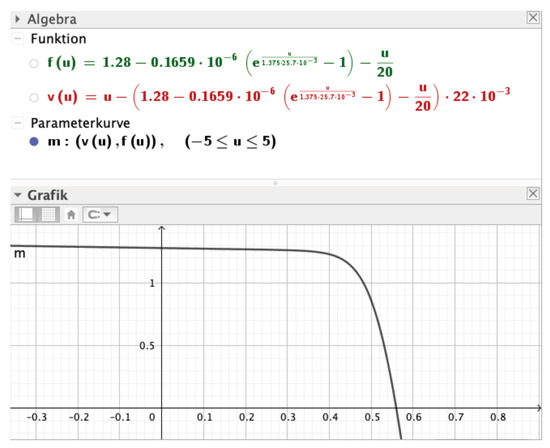
Figure 2. Curve $C_{IV}$ is situated in the first quadrant.

Next, we consider the PV module studied in [4]. It consists of 60 cells, and its data sheet specifies

$$I_{ph}\approx I_{sc,T_{STC}}=10.82 \mathrm{A}; \alpha =0.04\%{/}^{°}\mathrm{C}.$$

In their experiments, by combining numerical with analytical methods, the authors found

$$I_{0,T_{STC}}=4.17·{10}^{-8} \mathrm{A}; R_{s,T_{STC}}=0.0037\mathsf{\Omega }; R_{sh}=112.1\mathsf{\Omega }.$$

We picked the constant value $n=1.375$ for the diode ideality factor from a somewhat scattered cloud of measurements.

In addition to the declarations of these parameters, twelve lines of code are sufficient to generate an interactive worksheet in GeoGebra (We picked GeoGebra because it allows to manipulate dynamic geometric and algebraic objects in a very intuitive way. It is widely used in geometry research and teaching. Maple or Mathematica would be good alternatives) that draws the parameterized curve $C_{IV,t}$ depicted in Figure 3 and Figure 4, computes its MPP and the maximum power, $P_t$; some technical details are given in the Appendix A. The dashed (blue) curve is the hyperbola $I=h\left(V\right)=\frac{P_t}{V}$ consisting of all points $(V,I)$ in the plane for which $V·I$ equals maximum power; it touches $C_{IV,t}$ at MPP from the right-hand side.

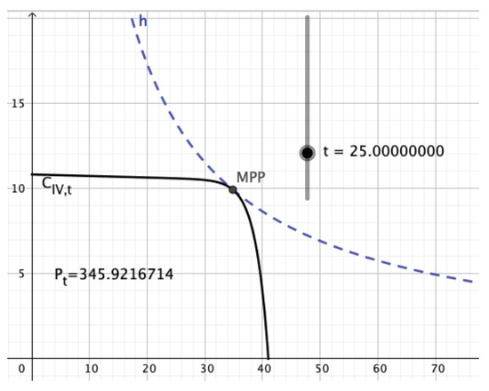
Figure 3. The slider allows temperature t to be changed between 0° and 100 °C.

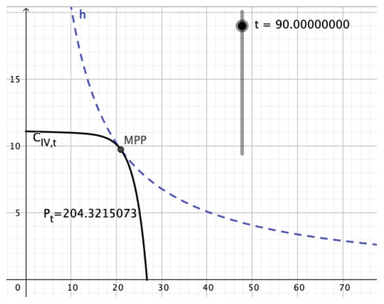
Figure 4. One can observe how curve $C_{IV}$ and its MPP change; number $P_t$ denotes the power at MPP.

In this example, it appears that the curvatures of $C_{IV}$ and h at MPP are, up to their opposite signs, closer at high temperature than at STC. This observation raises the question of whether errors in determining the exact MPP on $C_{IV}$ are more detrimental at lower temperature.

Finally, we want to explore what difference it makes to have $R_s$ linearly grow with T as opposed to fixing it at $R_{s,T_{STC}}$.

Figure 5 depicts the curves $C=C_{IV,t}$ for temperature-dependent resistor $R_s$, and $D=D_{IV,T_{STC}}$ for the constant value $R_{s,T_{STC}}$. One has to zoom in considerably to separate the two curves. Their maximum power values are quite close: $182.54$ W for C and $182.62$ W for D.

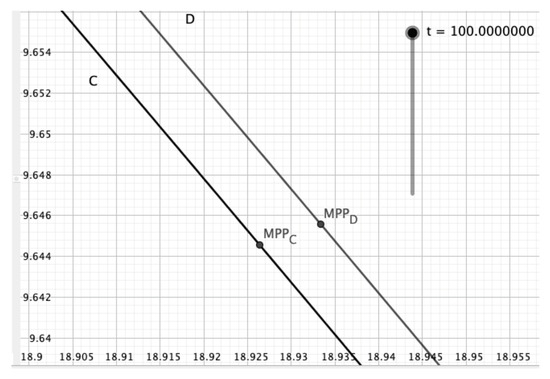
Figure 5. Curve $D=D_{IV,t}$ results from using constant series resistor $R_{s,T_{STC}}$, rather than having its value increase with factor $\frac{T}{T_{STC}}$, as with $C=C_{IV,t}$.

This can be explained by the following observation. Let $(V^C,I)$ denote a point on C. Then, $V^C$ and I satisfy Equation (3) with series resistor value $R_s$. Now, let us move this point a distance of $I·(R_s-R_{s,T_{STC}})$ to the right, as sketched in Figure 6, resulting in point $(V^D,I)$. Because of

$$\begin{array}{c}\hfill V^C+I·R_s=V^D+I·R_{s,T_{STC}}\end{array}$$

(23)

the new point also fulfills (3), but for resistor $R_{s,T_{STC}}$. Therefore, it must be situated on curve D. Consequently, the point on D to the right of $MP{P}_C$ in Figure 5 is just

$$\begin{array}{c}\hfill 9.645·(\frac{100+273.15}{25+273.15}-1)·0.0037=0.0089\left(V\right)\end{array}$$

(24)

away!

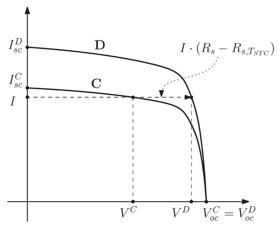
Figure 6. A sketch of two I–V curves $C,D$ in the single-diode model for series resistors $R_s>R_{s,T_{STC}}$, respectively, and identical parameters otherwise.

4. Discussion

We have introduced a new way to describe, in parameterized form, I–V curves for the single-diode, double-diode, and Bishop’s equivalent circuit models. The parameterization makes it possible to visualize I–V curves and their dependence on temperature interactively, using rather simple means. Extending this method to include variable irradiance or angle would be straightforward. We expect that our approach will help to provide new insights for the photovoltaic research community. As a side result, it could be beneficial for teaching solar systems at academic level.

References

- De Oliveira, O. The implicit and inverse function theorems: Easy proofs. Real Anal. Exch. 2014, 39, 207–218. [Google Scholar] [CrossRef]
- Quaschning, V. Simulation der Abschattungsverluste bei Solarelektrischen Systemen; Verlag Dr. Köster: Berlin, Germany, 1996; pp. 28–57. Available online: https://www.volker-quaschning.de/downloads/abschattungsverluste.pdf (accessed on 2 November 2022).
- Jain, A.; Kapoor, A. Exact analytical solutions of the parameters of real solar cells using Lambert W-function. Sol. Energy Mater. Sol. Cells 2004, 81, 269–277. [Google Scholar] [CrossRef]
- Spertino, F.; Malgaroli, G.; Amato, A.; Qureshi, M.A.E.; Ciocia, A.; Siddiqui, H. An Innovative technique for energy assessment of a highly efficient photovoltaic module. Solar 2022, 2, 321–333. [Google Scholar] [CrossRef]
- Ruschel, S.R.; Gasparin, F.P.; Krenzinger, A. Experimental analysis of the single diode model parameters dependence on irradiance and temperature. Sol. Energy 2021, 217, 134–144. [Google Scholar] [CrossRef]
- Durán, E.; Piliougine, M.; Sidrach-de-Cardona, M.; Galán, J.; Andújar, J.M. Different methods to obtain the I–V curve of PV modules: A review. In Proceedings of the IEEE Photovoltaic Conference, San Diego, CA, USA, 11–16 May 2008. [Google Scholar]
- Humada, A.M.; Hojabri, M.; Mekhilef, S.; Hamada, H.M. Solar sell parameters extraction based on single and double-diode models: A review. Renew. Sustain. Energy Rev. 2016, 56, 494–509. [Google Scholar] [CrossRef]
- Phang, J.C.H.; Chan, D.S.H.; Philips, J.R. Accurate analytical method for the extraction of solar cell parameters. Electron. Lett. 1984, 20, 406–408. [Google Scholar] [CrossRef]
- Chan, D.S.H.; Phang, J.C.H. Analytical methods for the extraction of solar-cell single- and double-diode model parameters from I–V characteristics. IEEE Trans. Electron Devices 1987, 34, 286–293. [Google Scholar] [CrossRef]
- De Soto, W.; Klein, S.A.; Beckman, W.A. Improvement and validation of a model for photovoltaic array performance. Sol. Energy 2006, 80, 78–88. [Google Scholar] [CrossRef]
Publisher’s Note: MDPI stays neutral with regard to jurisdictional claims in published maps and institutional affiliations. |
© 2022 by the author. Licensee MDPI, Basel, Switzerland. This article is an open access article distributed under the terms and conditions of the Creative Commons Attribution (CC BY) license (https://creativecommons.org/licenses/by/4.0/).