Dynamical System Stability Criteria Based on the Frobenius Norm

Abstract

It is well known that the position of the Jacobian matrix spectrum in the left-half complex plane provides the local asymptotic stability of a nonlinear dynamical system, but it is also well known that for large matrices, computing its eigenvalues just to see their position is computationally prohibitive. Instead, it is recommended to check if a given matrix belongs to the H-matrix class and has negative diagonal entries. Since confirming the H-matrix property is computationally costly, the preference is to work with its subclasses, which are defined by simpler conditions. In this paper, we develop and investigate a new subclass of H-matrices via the Frobenius matrix norm, which generalizes the recently introduced classes. We support its significance with real-life examples and clarify its relationship to some well-known block H-matrices based on the Euclidean matrix norm. The main novelty in this paper is that when a fast and inexpensive answer about the stability of a dynamical system is required, and the system matrix has a natural block structure, we develop a simple tool to check whether this structure, along with the additional condition of negative diagonal elements, ensures stability. This is especially important when the matrix does not belong to any previously known H-matrix subclasses.

1. Introduction

The significance of the concept of block matrices is justified by the fact that many application problems in various settings initially possess special structures, which speak in favor of an interplay within interacting groups, as well as the interlinkage of groups as a whole (structured networks). Taking into consideration the high dimensionality of such systems, the possibility of finding a procedure that would optimize the problem in terms of the working dimension and adapt it to the computational capacities without losing the information contained in it, the commitment to this topic becomes even greater. Finally, many computational procedures, such as the discretization of partial differential equations, via the finite element method or finite difference method, produce matrices with block structures. Other times, it is also useful to divide matrices without a predetermined block structure, for example, a full matrix, into blocks and enable their study, which is perhaps unavailable when observed in the point-wise case. Some pioneer steps toward responding to block necessity occurred in the second half of the previous century [1,2,3,4].

In the theory of dynamical systems and the investigation of their stability, it is desirable to conclude that the corresponding matrix belongs to the class of H-matrices. If, in addition, this matrix has all diagonal entries negative, then the observed dynamical system is locally stable. However, determining whether a certain matrix is an H-matrix in the first place is a challenge itself. How to check if a given matrix is an H-matrix is important, but it is still an open question. A well-known characterization of H-matrices is given by the fact that the matrix is an H-matrix if and only if it can be scaled to a strictly diagonally dominant ($SDD$) matrix by a nonsingular diagonal matrix (from the right-hand side). The real challenge is how to find such a scaling matrix. Hence, finding new subclasses of H-matrices is still very desirable, in particular the subclasses of H-matrices to which the membership is straightforwardly confirmable. The extensive literature on this topic recognizes subclasses defined by conditions that are a kind of generalization of strict diagonal dominance; for a thorough recapitulation, see [5,6,7,8,9,10,11,12,13,14,15,16], and for the most recent ones, see [17,18,19].

What all these classes have in common is the infinity norm underlying them. In a real-life model, for example from ecology or epidemiology, this matrix norm may be interpreted as a measure which captures the individual strengths of interactions within every functional group level (row) with respect to other levels (columns). However, a more comprehensive approach that takes into account the aggregate interactions of all functional groups (the entire structure, or its key parts) has been presented in a recently published paper [20] and involves the use of the Euclidean vector and Frobenius matrix norms as well as the partition of the index set into two subsets. Here, we will present a generalization of that class to an arbitrary partition of the set of indices into ℓ subsets, i.e., a representation of the matrix in $\mathsf{\ell }\times \mathsf{\ell }$ block form. Additionally, we will compare this approach with the classic block approach used in [21].

The paper is organized as follows. Section 2 contains notations and preliminary background. Section 3 reveals the new subclass of H-matrices, a further block generalization of matrices studied in [20], using the Frobenius norm. In Section 4, we investigate the connection between our new class and the known block H-matrices, which were researched in [21]. We justify the usefulness of the proposed class in Section 5, where two practical examples are provided—one from the modeling of infectious diseases and the other from the ecological modeling of soil food webs. Section 6 reveals comments on the possible approach using other matrix norms, and we bring our paper to an end in Section 7 with some concluding remarks.

2. Notations and Preliminaries

Although they are well known, here we recall the usual notations. For an arbitrary matrix $A=\left[a_{ij}\right]\in {\mathbb{C}}^{n,n}$, we define $N:=\{1,2,\dots ,n\}$ as the set of indices of $A,$ the quantities

$${\displaystyle r_i\left(A\right):=\sum _{j\in N\setminus \left\{i\right\}}\left|a_{ij}\right|, i\in N}$$

(1)

as the i-th deleted absolute row sums and $\pi ={\left\{p_j\right\}}_{j=0}^{\mathsf{\ell }}$ as a partition of the index set N, where the non-negative numbers $p_j, j=1,2,\dots ,\mathsf{\ell }$, satisfy the following criteria

$$p_0:=0<p_1<p_2<\dots <p_{\mathsf{\ell }}:=n.$$

Given a partition $\pi ={\left\{p_j\right\}}_{j=0}^{\mathsf{\ell }}$, an $n\times n$ matrix A is partitioned into $\mathsf{\ell }\times \mathsf{\ell }$ blocks,

$$A=\left[\begin{array}{cccc}{A}_{11}& A_{12}& \dots & A_{1\mathsf{\ell }}\\ A_{21}& A_{22}& \dots & A_{2\mathsf{\ell }}\\ ⋮& ⋮& \ddots & ⋮\\ A_{\mathsf{\ell }1}& A_{\mathsf{\ell }2}& \dots & A_{\mathsf{\ell }\mathsf{\ell }}\end{array}\right]={\left[A_{ij}\right]}_{\mathsf{\ell }\times \mathsf{\ell }}.$$

(2)

The notation ${\parallel ·\parallel }_{\infty }$ is interchangeably used in order to refer to the vector infinity norm and the matrix norm induced by it:

$${\parallel x\parallel }_{\infty }=\underset{i\in N}{max}|x_i{|,\hspace{1em}\parallel A\parallel }_{\infty }=\underset{i\in N}{max}\sum _{j\in N}\left|a_{ij}\right|.$$

We use ${\parallel ·\parallel }_2$ to denote the Euclidean vector or matrix norm, which are respectively defined as follows:

$${\parallel x\parallel }_2=\sqrt{\sum _{i\in N}{\left|x_i\right|}^2}, {\parallel A\parallel }_2=\sqrt{\rho \left(A^{H}A\right)}=\sqrt{\rho \left(A{A}^H\right)},$$

with $\rho \left(B\right)$ representing the spectral radius of $B,$ i.e., the maximal eigenvalue of B taken by moduli. Let us also recall that both Euclidean vectors and matrix norms satisfy the monotonicity property, i.e.,

$$0\le x\le y⟹{\parallel x\parallel }_2\le {\parallel y\parallel }_{2}andO\le A\le B⟹{\parallel A\parallel }_2\le {\parallel B\parallel }_2.$$

(3)

With ${\parallel ·\parallel }_F$, we refer to the Frobenius matrix norm, which is given by

$${\parallel A\parallel }_F=\sqrt{\sum _{i=1}^n\sum _{j=1}^n{\left|a_{ij}\right|}^2}=\sqrt{tr\left(A^{H}A\right)}=\sqrt{tr\left(A{A}^H\right)},$$

where $tr\left(B\right)$ is the trace of B, which is the sum of its diagonal entries. Obviously, the Frobenius matrix norm is also monotonic.

For any $n\times n$ matrix A partitioned into $\mathsf{\ell }\times \mathsf{\ell }$ blocks in a style proposed by (2) and a matrix norm ${\parallel ·\parallel }_{\left(m\right)}$, we introduce a real-valued $\mathsf{\ell }\times \mathsf{\ell }$ auxiliary matrix:

$$N_{\left(m\right)}\left(A\right)=\left[\begin{array}{cccc}\parallel A_{11}{\parallel }_{\left(m\right)}& \parallel A_{12}{\parallel }_{\left(m\right)}& \dots & \parallel A_{1\mathsf{\ell }}{\parallel }_{\left(m\right)}\\ \parallel A_{21}{\parallel }_{\left(m\right)}& \parallel A_{22}{\parallel }_{\left(m\right)}& \dots & \parallel A_{2\mathsf{\ell }}{\parallel }_{\left(m\right)}\\ ⋮& ⋮& \ddots & ⋮\\ \parallel A_{\mathsf{\ell }1}{\parallel }_{\left(m\right)}& \parallel A_{\mathsf{\ell }2}{\parallel }_{\left(m\right)}& \dots & \parallel A_{\mathsf{\ell }\mathsf{\ell }}{\parallel }_{\left(m\right)}\end{array}\right].$$

(4)

Finally, we recall some well-known (point-wise) classes of matrices. To begin with, a matrix $A=\left[a_{ij}\right]\in {\mathbb{R}}^{n,n}$ is said to be a nonsingular M-matrix if it is a Z-matrix (i.e., $a_{ii}>0$ and $a_{ij}\le 0$ for all $i\ne j$), nonsingular, and its inverse is entrywise non-negative: $A^{-1}\ge O$.

H-matrices are defined as matrices $A=\left[a_{ij}\right]\in {\mathbb{C}}^{n,n}$ whose comparison matrix

$$\mathcal{M}\left(A\right)=\left[{\alpha }_{ij}\right]\in {\mathbb{R}}^{n,n}, {\alpha }_{ij}=\left\{\begin{array}{cc} |a_{ii}|,\hfill & i=j\hfill \\ -|a_{ij}|,\hfill & i\ne j\hfill \end{array}\right.$$

is a nonsingular M-matrix, i.e., $\mathcal{M}{\left(A\right)}^{-1}\ge O$. It is well known that every H-matrix is nonsingular. Throughout the paper, we only deal with nonsingular M-matrices, so we will call them, simply, M-matrices.

Determining whether a matrix is an H-matrix can be computationally expensive. Thus, a practical alternative is to identify as many subclasses of H-matrices as possible, which are characterized by simple and easily testable conditions on their elements, c.f. [5,6,7,8,9,10,11,12,16,20].

The most famous subclass of H-matrices is the class of strictly diagonally dominant ($SDD$) matrices [9] that contains all matrices $A=\left[a_{ij}\right]\in {\mathbb{C}}^{n,n}$ meeting the property

$$|a_{ii}| >r_i\left(A\right) \mathrm{for} \mathrm{all} i\in N.$$

Another important H-matrix subclass was introduced in [7], where for a proper nonempty subset S of the index set N and its complement, $\overline{S}:=N\setminus S$, the sum of moduli of off-diagonal entries in each row (1) is split into two parts:

$$r_i\left(A\right)=r_i^S\left(A\right)+r_i^{\overline{S}}\left(A\right),$$

where

$${\displaystyle r_i^S\left(A\right):=\sum _{j\in S\setminus \left\{i\right\}}\left|a_{ij}\right|and{r}_i^{\overline{S}}\left(A\right):=\sum _{j\in \overline{S}\setminus \left\{i\right\}}\left|a_{ij}\right|.}$$

Then, a matrix $A\in {\mathbb{C}}^{n,n},$$n\ge 2,$ is called an $S-SDD$ matrix, provided that for a given nonempty proper subset S of the set of indices N and for every $i\in S$ and every $j\in \overline{S},$ the following two conditions hold simultaneously:

$$\begin{array}{cc}|a_{ii}|>r_i^S\left(A\right),\hfill & \hspace{1em}\hspace{1em}\hspace{1em}\hspace{1em}\hspace{1em}\hspace{1em}\hspace{1em}\hspace{1em}\hspace{1em}\hspace{1em} \hfill \end{array}$$

(5)

$$\left(|a_{ii}|-r_i^S\left(A\right)\right)\left(|a_{jj}|-r_j^{\overline{S}}\left(A\right)\right)>r_i^{\overline{S}}\left(A\right)r_j^S\left(A\right).$$

(6)

Therefore, $SDD$ matrices can be viewed as a limit case when $S=N.$

In the dynamical analysis of linear and nonlinear dynamical systems, the stability stands out as one of the most significant properties. The traditional technique of assessing stability is in line with the Routh–Hurwitz criterion and uses the knowledge about the position of the spectrum—whether all eigenvalues are located in the open left half-plane or not. But since this approach is translated into a polynomial problem, it becomes too expensive for higher-order systems. Lemma 1 from [20], which is closely connected to the Minimal Geršgorin set, may serve as a practical tool in providing answers about stability.

Lemma 1.

If $A\in {\mathbb{C}}^{n,n}$ is an H-matrix with negative diagonal entries, then the spectrum of A lies in ${\mathbb{C}}^{-}$.

It is worth mentioning that due to obvious computational costs, we never examine this property by definition but rather check whether the matrix belongs to some subclass of H-matrices.

3. A New Subclass of H-Matrices

In the course of this paper, $A=D-B$ will be the standard splitting of a matrix A into its diagonal $D=diag(a_{11},a_{22},\dots ,a_{nn})$ and off-diagonal ($-B$) part. Additionally, we will use the notation

$$J\left(A\right):=D^{-1}B,$$

and whenever there is no chance of a misinterpretation, we will denote it as $J:=J\left(A\right)$.

The main motivation to introduce the $SD{D}_F$ matrix class in [20] was the characterization of the well-known $SDD$ matrices as matrices for which ${\parallel J\parallel }_{\infty }<1$. Namely, in that paper, $SD{D}_F$ matrices were defined by the condition ${\parallel J\parallel }_F<1$. In a similar way, in the same paper, $S-SDD$ matrices were a motivation for defining $S-SD{D}_F$ matrices. Here, we aim to make one step forward and allow the matrix to be partitioned into more than two blocks.

For any block matrix $A={\left[A_{ij}\right]}_{\mathsf{\ell }\times \mathsf{\ell }}$ of the form (2), with all diagonal entries nonzero, we will apply the same partition to $J=J\left(A\right)$:

$$J=\left[\begin{array}{cccc}{J}_{11}& J_{12}& \dots & J_{1\mathsf{\ell }}\\ J_{21}& J_{22}& \dots & J_{2\mathsf{\ell }}\\ ⋮& ⋮& \ddots & ⋮\\ J_{\mathsf{\ell }1}& J_{\mathsf{\ell }2}& \dots & J_{\mathsf{\ell }\mathsf{\ell }}\end{array}\right].$$

(7)

Finally, we use J to define a special comparison matrix

$$A_F^{\pi }=I-N_F\left(J\right).$$

Our new class of matrices is defined in the following way.

Definition 1.

A matrix $A=\left[a_{ij}\right]\in {\mathbb{C}}^{n,n}$ of the block form (2), with nonzero diagonal entries, is called an $H_F^{\pi }$-matrix provided that its comparison matrix $A_F^{\pi }$ is an M-matrix.

Before we prove that this class is a subclass of H-matrices, let us illustrate a step-by-step calculation of $A_F^{\pi }$ on a worked-out small numerical example, according to the Algorithm 1.

Algorithm 1 Calculation of $A_F^{\pi }$

Input: matrix $A,$ partition $\pi$

1: Split A into diagonal part D and off-diagonal part $-B:$$A=D-B$

2: Compute $J=D^{-1}B$

3: Partition J into blocks according to partition $\pi$

4: Calculate the Frobenius norms of each block to get $N_F\left(J\right)$

5: Compute $A_F^{\pi }=I-N_F\left(J\right)$

Output: matrix $A_F^{\pi }$

$$A=\left[\begin{array}{ccccccc}11& -2& 1& -3& -2& -1& 2\\ 3& 21& 2& -1& -3& 2& -1\\ -1& -2& 22& 3& 1& 2& 3\\ 2& -1& -2& 21& -3& -1& 2\\ 3& 2& 1& -2& 23& -3& -1\\ -1& -3& -2& 1& -2& 19& 3\\ 2& -1& 3& 1& 2& -2& 20\end{array}\right] \mathrm{and} \pi =\{0,2,5,7\}.$$

First, we split $A=D-B,$ where

$$D=\left[\begin{array}{ccccccc}11& 0& 0& 0& 0& 0& 0\\ 0& 21& 0& 0& 0& 0& 0\\ 0& 0& 22& 0& 0& 0& 0\\ 0& 0& 0& 21& 0& 0& 0\\ 0& 0& 0& 0& 23& 0& 0\\ 0& 0& 0& 0& 0& 19& 0\\ 0& 0& 0& 0& 0& 0& 20\end{array}\right] \mathrm{and} B=D-A.$$

Next, we calculate $J=D^{-1}B:$

$$J=\left[\begin{array}{ccccccc}0& 0.18& -0.09& 0.27& 0.18& 0.09& -0.18\\ -0.14& 0& -0.1& 0.05& 0.14& -0.1& 0.05\\ 0.05& 0.09& 0& -0.14& -0.05& -0.09& -0.14\\ -0.1& 0.05& 0.1& 0& 0.14& 0.05& -0.1\\ -0.13& -0.09& -0.04& 0.09& 0& 0.13& 0.04\\ 0.05& 0.16& 0.11& -0.05& 0.11& 0& -0.16\\ -0.1& 0.05& -0.15& -0.05& -0.1& 0.1& 0\end{array}\right],$$

from whence, with respect to partition $\pi =\{0,2,5,7\},$ we calculate the Frobenius norms of each of nine blocks and obtain the following:

$$N_F\left(J\right)=\left[\begin{array}{ccc}0.23& 0.38& 0.23\\ 0.22& 0.25& 0.24\\ 0.2& 0.25& 0.19\end{array}\right] \mathrm{and} A_F^{\pi }=\left[\begin{array}{ccc}0.77& -0.38& -0.23\\ -0.22& 0.75& -0.24\\ -0.2& -0.25& 0.81\end{array}\right].$$

Now, we prove the following theorem.

Theorem 1.

Every $H_F^{\pi }$-matrix is nonsingular. Moreover, it is an H-matrix.

Proof. 

Let A be an $H_F^{\pi }$-matrix. Then, D is a nonsingular matrix. To prove its nonsingularity, suppose, on the contrary, that there exists a vector $x\in {\mathbb{C}}^n$, $x\ne 0$, such that $Ax=0$, which means that $(D-B)x=0$, i.e., $x=Jx.$ Using the same partition $\pi ,$ let x be partitioned as $x={[X_1,\dots ,X_{\mathsf{\ell }}]}^T$, and the set of indices $N=\{1,2,\dots ,n\}$ be partitioned to ℓ consecutive subsets $N_1,N_2,\dots ,N_{\mathsf{\ell }}$, such that indices related to $X_i$ form the subset $N_i$. Then, for all $k=1,2,\dots ,\mathsf{\ell }$ we have that

$$X_k=\sum _{t=1}^{\mathsf{\ell }}{J}_{kt}{X}_t,$$

from where, after applying the Euclidean vector norm to both sides of the latter equations and knowing that Frobenius matrix norm is consistent with this vector norm, we obtain

$$\parallel X_k{\parallel }_2\le \sum _{t=1}^{\mathsf{\ell }}\parallel J_{kt}{\parallel }_F{\parallel X_t\parallel }_2.$$

in mind that

$$\parallel X_k{\parallel }_2={\left(I\left[\begin{array}{c}\parallel X_1{\parallel }_2\\ ⋮\\ \parallel X_{\mathsf{\ell }}{\parallel }_2\end{array}\right]\right)}_k and \sum _{t=1}^{\mathsf{\ell }}\parallel J_{kt}{\parallel }_F{\parallel X_t\parallel }_2={\left(N_F\left(J\right)\left[\begin{array}{c}\parallel X_1{\parallel }_2\\ ⋮\\ \parallel X_{\mathsf{\ell }}{\parallel }_2\end{array}\right]\right)}_k,$$

the above inequality can be rewritten as

$${\left((I-N_F\left(J\right))\left[\begin{array}{c}\parallel X_1{\parallel }_2\\ ⋮\\ \parallel X_{\mathsf{\ell }}{\parallel }_2\end{array}\right]\right)}_k\le 0, \mathrm{for} \mathrm{every} k=1,2,\dots ,\mathsf{\ell }.$$

If we define an auxiliary vector $\theta$ as follows, then the last statement gives exactly

$$\theta :=A_F^{\pi }\left[\begin{array}{c}\parallel X_1{\parallel }_2\\ ⋮\\ \parallel X_{\mathsf{\ell }}{\parallel }_2\end{array}\right]\le 0.$$

Finally, the assumption that $A_F^{\pi }$ is a nonsingular M-matrix guarantees that ${\left(A_F^{\pi }\right)}^{-1}\ge O$, thus

$$\left[\begin{array}{c}\parallel X_1{\parallel }_2\\ ⋮\\ \parallel X_{\mathsf{\ell }}{\parallel }_2\end{array}\right]={\left(A_F^{\pi }\right)}^{-1}\theta \le 0.$$

This is an obvious contradiction with $x\ne 0$, so the first part of the proof is concluded.

Now, we will prove that A is an H-matrix, i.e., that $\mathcal{M}\left(A\right)$ is an M-matrix. In order to do that, for $\mathcal{M}\left(A\right)$, use the standard splitting $\mathcal{M}\left(A\right)=\left|D\right|-\left|B\right|$ into its diagonal and off-diagonal part. Obviously, $\mathcal{M}\left(A\right)$ is a Z-matrix, so it remains to prove that $\mathcal{M}\left(A\right)$ is nonsingular and ${\left(\mathcal{M}\left(A\right)\right)}^{-1}\ge O$. At first, note that

$$J\left(\mathcal{M}\left(A\right)\right)={\left|D\right|}^{-1}\left|B\right|=|D^{-1}B|=|J\left(A\right)|,\hspace{1em}\mathrm{and}\hspace{1em}{N}_F\left(J\left(\mathcal{M}\left(A\right)\right)\right)=N_F\left(J\left(A\right)\right).$$

To that end, consider the following auxiliary matrix

$$C\left(\lambda \right):=\lambda \left|D\right|-\left|B\right|.$$

If $\lambda$ is an arbitrary eigenvalue of ${\left|D\right|}^{-1}\left|B\right|$, then $C\left(\lambda \right)$ is singular, which becomes obvious from

$$C\left(\lambda \right)=\left|D\right|(\lambda I-|D{|}^{-1}\left|B\right|).$$

On the other hand,

$$J\left(C\left(\lambda \right)\right)={\left(\lambda \left|D\right|\right)}^{-1}\left|B\right|={\displaystyle \frac{1}{\lambda }}{\left|D\right|}^{-1}\left|B\right|={\displaystyle \frac{1}{\lambda }}J\left(\mathcal{M}\left(A\right)\right), \mathrm{hence}$$

$$C{\left(\lambda \right)}_F^{\pi }=I-N_F\left(J\left(C\left(\lambda \right)\right)\right)=I-N_F\left({\displaystyle \frac{1}{\lambda }}J\left(\mathcal{M}\left(A\right)\right)\right)=I-{\displaystyle \frac{1}{\left|\lambda \right|}}{N}_F\left(J\left(A\right)\right),$$

so if $\left|\lambda \right|\ge 1$, then $C{\left(\lambda \right)}_F^{\pi }\ge A_F^{\pi }$, which means that $C{\left(\lambda \right)}_F^{\pi }$ (being a Z matrix) is a nonsingular M-matrix, too. But then $C\left(\lambda \right)$ is an $H_F^{\pi }$-matrix and, therefore, nonsingular. Obviously, both assumptions, the first that $\lambda$ is an eigenvalue of ${\left|D\right|}^{-1}\left|B\right|$, and the second that $\left|\lambda \right|\ge 1$, cannot be simultaneously satisfied, since they lead to an obvious contradiction. Hence, moduli of all eigenvalues of ${\left|D\right|}^{-1}\left|B\right|$ are strictly less than 1, i.e., $\rho \left(\right|D{|}^{-1}\left|B\right|)<1$ which implies that $I-{\left|D\right|}^{-1}\left|B\right|$ is a nonsingular matrix. But, then $\left|D\right|\left(I-{\left|D\right|}^{-1}\left|B\right|\right)=\left|D\right|-\left|B\right|=\mathcal{M}\left(A\right)$ is also a nonsingular matrix. The last step is to assert that ${\left(\mathcal{M}\left(A\right)\right)}^{-1}\ge O$. Indeed,

$${\left(\mathcal{M}\left(A\right)\right)}^{-1}=\left(\right|D\left|\right(I-{\left|D\right|}^1{\left|B\right|\left)\right)}^{-1}=\sum _{k=0}^{\infty }{\left(\right|D|}^{-1}{\left|B\right|)}^k{\left|D\right|}^{-1}\ge O,$$

which means that $\mathcal{M}\left(A\right)$ is an M-matrix, i.e., A is an H-matrix, which completes the proof. □

Taking Lemma 1 into account, we immediately formulate the subsequent

Corollary 1.

If $A\in {\mathbb{C}}^{n,n}$ is an $H_F^{\pi }$-matrix with negative diagonal entries, then the spectrum of A lies in ${\mathbb{C}}^{-}$.

Remark 1.

The definition of $H_F^{\pi }$ matrices requires a validation if $A_F^{\pi }$ is an M-matrix. In practice, this is usually performed not directly via the definition of M-matrices (requiring invertibility) but rather using the fact that any (real-valued) Z-matrix, which is defined by easily checkable, entry-wise dependent criteria (such as SDD, S-SDD, etc.), is an M-matrix.

Remark 2.

For a very specific choice, $\pi =\{0,n\}$, our new class becomes the SDD_F class from [20], which is defined by

$${\parallel J\parallel }_F<1.$$

Remark 3.

When considering the special case $\pi =\{0,k,n\}$, our class becomes defined by the criterion

$$A_F^{\pi }=I-\left[\begin{array}{cc}\parallel J_{11}{\parallel }_F& \parallel J_{12}{\parallel }_F\\ \parallel J_{21}{\parallel }_F& \parallel J_{22}{\parallel }_F\end{array}\right]\hspace{1em}\mathrm{is}\mathit{an}M-\mathit{matrix}.$$

In the case where we select $S=\{1,2,\dots ,k\}$, with k being the dimension of $J_{11}$, one can validate that our class becomes equivalent to the $S-$SDD_F class defined in [20]:

$$\begin{array}{cc}\parallel J_{11}{\parallel }_F<1,\hfill & \hfill \hspace{1em}\hspace{1em}\hspace{1em}\hspace{1em}\hspace{1em}\hspace{1em}\hspace{1em}\hspace{1em}\hspace{1em}\end{array}$$

(8)

$$\left(1-\parallel J_{11}{\parallel }_F\right)\left(1-\parallel J_{22}{\parallel }_F\right)>\parallel J_{12}{\parallel }_F{\parallel J_{21}\parallel }_F.$$

(9)

Namely, conditions (8) and (9) combined imply that diagonal elements of $A_F^{\pi }$ are positive, while condition (9) translates that $A_F^{\pi }$ is a doubly strictly diagonally dominant matrix [11], hence being an M-matrix. For the reverse direction, assuming that $A_F^{\pi }$ is an M-matrix, guarantees that (8) is satisfied and that there exists $\gamma >0$ such that

$$A_F^{\pi }\left[\begin{array}{c}\hfill 1\\ \hfill \gamma \end{array}\right]>0,$$

which means that

$$\left(1-\parallel J_{11}{\parallel }_F\right)-\gamma \parallel J_{12}{\parallel }_F>0\hspace{1em}and\hspace{1em}-{\parallel J_{21}\parallel }_F+\gamma \left(1-\parallel J_{22}{\parallel }_F\right)>0.$$

Whenever $\parallel J_{12}{\parallel }_F{\parallel J_{21}\parallel }_F=0$, the inequality (9) holds trivially, otherwise

$$\gamma <{\displaystyle \frac{1-\parallel J_{11}{\parallel }_F}{\parallel J_{12}{\parallel }_F}}\hspace{1em}and\hspace{1em}\gamma >{\displaystyle \frac{\parallel J_{21}{\parallel }_F}{1-\parallel J_{22}{\parallel }_F}},$$

from whence

$${\displaystyle \frac{\parallel J_{21}{\parallel }_F}{1-\parallel J_{22}{\parallel }_F}}<{\displaystyle \frac{1-\parallel J_{11}{\parallel }_F}{\parallel J_{12}{\parallel }_F}},$$

which is exactly condition (9).

Remark 4.

Finally, if one chooses another very specific case, $\pi =\{0,1,2,\dots ,n\}$ which is the singleton partition, then

$${\left(A_F^{\pi }\right)}_{ij}=\left\{\begin{array}{cc} 1,\hfill & i=j\hfill \\ -{\displaystyle \frac{|a_{ij}|}{|a_{ii}|}},\hfill & i\ne j\hfill \end{array}\right.$$

from where we can see that $A_F^{\pi }=\mathcal{D}·\mathcal{M}\left(\mathcal{A}\right),$ where $\mathcal{D}={\left|D\right|}^{-1}.$ So, for the singleton partition, it is obvious that our new class is actually the H-matrix class itself.

Remark 5.

Similarly, as it has been ascertained in [20], one can conclude that our new subclass of H-matrices holds a general position relative to all known H-matrix subclasses based on the infinity norm.

If one would like to clarify the relationship among the classes using a schematic diagram, it shall be kept in mind that the index subset S is fixed for the $S-SD{D}_F$ class, just as partition $\pi$ is fixed for the $H_F^{\pi }$ class. Provided that partition $\pi$ divides the index set exactly into S and $\overline{S},$ these classes are precisely the same; see Remark 3. Should we, on the other hand, define the following classes of matrices:

• $CKV$ class: all matrices for which there exists an index subset S, such that matrix is $S-SDD$ (please note that this term was established in [5]);
• $PartH$ class: all matrices for which there exists a partition $\pi$, such that matrix is $H_F^{\pi }$ (this term we only introduce temporarily).

Then, $CKV$ is certainly contained in $PartH$, because $PartH$ is actually the H-matrix class, according to Remark 4. The relationship among classes defined via the Frobenius norm and the ones defined via the infinity norm is general, which is pointed out in Remark 5. For a fixed subset S, and very often the choice of S is imposed by the matrix itself, the $S-SDD$ and and $S-SD{D}_F$ classes also stand in a general position. All the previously discussed relationships are illustrated using the diagram in Figure 1.

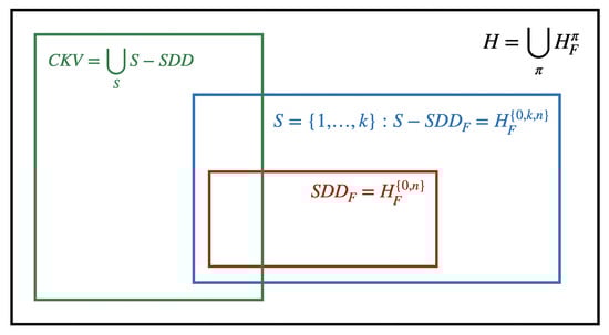
Figure 1. The relationship among $H,$ $CKV,$ $S-SD{D}_F$ and $SD{D}_F$ classes.

4. Relationship with Some Known Block H-Matrix Classes

In this section, we will investigate and establish the position that our new class of $H_F^{\pi }$-matrices takes in relation to the known class of block H-matrices, which was defined via the Euclidean matrix norm. More precisely, two such classes had been defined and studied in [21], so we preserve the assumptions and notations as follows. Under the assumption that each of the diagonal blocks of A is a nonsingular matrix, one is able to define comparison matrices in two different ways, following the style introduced in [22]:

$${⟨A⟩}_2^{\pi }=\left[\begin{array}{cccc}\parallel A_{11}^{-1}{\parallel }_2^{-1}& -\parallel A_{12}{\parallel }_2& \dots & -\parallel A_{1\mathsf{\ell }}{\parallel }_2\\ -\parallel A_{21}{\parallel }_2& \parallel A_{22}^{-1}{\parallel }_2^{-1}& \dots & -\parallel A_{2\mathsf{\ell }}{\parallel }_2\\ ⋮& ⋮& \ddots & ⋮\\ -\parallel A_{\mathsf{\ell }1}{\parallel }_2& -\parallel A_{\mathsf{\ell }2}{\parallel }_2& \dots & \parallel A_{\mathsf{\ell }\mathsf{\ell }}^{-1}{\parallel }_2^{-1}\end{array}\right],$$

or like it was proposed in [23]:

$${⟩A⟨}_2^{\pi }=\left[\begin{array}{cccc}1& -\parallel A_{11}^{-1}{A}_{12}{\parallel }_2& \dots & -\parallel A_{11}^{-1}{A}_{1\mathsf{\ell }}{\parallel }_2\\ -\parallel A_{22}^{-1}{A}_{21}{\parallel }_2& 1& \dots & -\parallel A_{22}^{-1}{A}_{2\mathsf{\ell }}{\parallel }_2\\ ⋮& ⋮& \ddots & ⋮\\ -\parallel A_{\mathsf{\ell }\mathsf{\ell }}^{-1}{A}_{\mathsf{\ell }1}{\parallel }_2& -\parallel A_{\mathsf{\ell }\mathsf{\ell }}^{-1}{A}_{\mathsf{\ell }2}{\parallel }_2& \dots & 1\end{array}\right].$$

One can easily confirm that

$$\mathrm{diag}\left(\parallel A_{11}^{-1}{\parallel }_2,\dots ,{\parallel A_{\mathsf{\ell }\mathsf{\ell }}^{-1}\parallel }_2\right)·{⟨A⟩}_2^{\pi }\le {⟩A⟨}_2^{\pi }.$$

(10)

For a given partition $\pi$, block matrix $A={\left[A_{ij}\right]}_{\mathsf{\ell }\times \mathsf{\ell }}$ is called one of the following:

• EBlock^π$H$-matrix if its comparison matrix ${⟨A⟩}_2^{\pi }$ is an M-matrix.
• eBlock^π$H$-matrix if its comparison matrix ${⟩A⟨}_2^{\pi }$ is an M-matrix.

With relation (10) kept in mind, and the definitions of EBlock^π and eBlock^πH-matrices, the following relationship is clear:

$$E{\mathrm{Block}}^{\pi }H\subset e{\mathrm{Block}}^{\pi }H.$$

One of the results presented by authors in [21] was that every eBlock^π$H$-matrix is nonsingular, implying the nonsingularity of all of the above-mentioned classes. But one has to keep in mind that, in general, these classes are not subclasses of (point-wise) nonsingular H-matrices—a statement which can be supported by the simple fact that a matrix $A={\left[a_{ij}\right]}_{n\times n}$ of the block form (2) can be an EBlock^π$H$- or eBlock^π$H$-matrix, while its diagonal entries are allowed to be zero—putting such a matrix outside the point-wise H-matrix class.

Having our new class of matrices in mind, we can now clarify its relationship to EBlock^π$H$ and eBlock^π$H$-matrices.

4.1. Relationship with EBlock^π$H$-Matrices

Let us consider the following matrix:

$$A_1=\left[\begin{array}{cccccc}4.08& 0.08& -0.19& -0.02& -0.48& -0.15\\ 0.11& 4.04& -0.05& -0.16& -0.16& -0.24\\ -0.24& -0.11& 0.05& 0& -0.02& 0\\ -0.2& -0.47& 0& 5& -0.2& -0.16\\ -0.19& -0.18& -0.08& -0.02& 3.98& -0.16\\ -0.49& -0.5& -0.45& -0.46& -0.07& 3.91\end{array}\right].$$

On the one hand, matrix $A_1$ belongs to $H_F^{\pi }$ class upon choosing $\pi =\{0,2,4,6\},$ but it is not an $E{\mathrm{Block}}^{\pi }H$-matrix for that same partition. Indeed, the comparison matrices are

$${\left(A_1\right)}_F^{\pi }=\left[\begin{array}{ccc}0.9664& -0.0626& -0.1424\\ -5.2811& 1& -0.4033\\ -0.1907& -0.1659& 0.956\end{array}\right]\mathrm{and}{⟨A_1⟩}_2^{\pi }=\left[\begin{array}{ccc}3.9629& -0.2137& -0.5561\\ -0.5508& 0.05& -0.2566\\ -0.7473& -0.6473& 3.825\end{array}\right].$$

Matrix ${\left(A_1\right)}_F^{\pi }$ is a Z-matrix and taking $x={[3,18,5]}^T,$ vector ${\left(A_1\right)}_F^{\pi }x$ is also positive, which means that ${\left(A_1\right)}_F^{\pi }$ is an M-matrix, whereas $det\left({⟨A_1⟩}_2^{\pi }\right)=-0.6106;$ therefore, ${⟨A_1⟩}_2^{\pi }$ can not be an M-matrix.

On the other hand, matrix $A_2$ is an H-matrix and it also belongs to the $E{\mathrm{Block}}^{\pi }H$ class for $\pi =\{0,2,4,6\},$ whilst it fails to become $H_F^{\pi }$ for that partition:

$$A_2=\left[\begin{array}{cccccc}14& -3& -1& -2& -1& -3\\ -1& 12& -1& -5& -3& -1\\ 0& -5& 11& -4& 0& -1\\ -2& 0& -3& 13& -1& 0\\ -1& -2& 0& -1& 6& -1\\ -3& 0& -2& 0& -1& 8\end{array}\right].$$

As a matter of fact, the comparison matrices are

$${\left(A_2\right)}_F^{\pi }=\left[\begin{array}{ccc}0.7701& -0.4539& -0.3471\\ -0.4799& 0.5693& -0.1191\\ -0.5287& -0.3005& 0.7917\end{array}\right]\mathrm{and}{⟨A_2⟩}_2^{\pi }=\left[\begin{array}{ccc}10.8023& -5.5414& -4\\ -5& 8.3704& -1\\ -3.2566& -2& 5.5858\end{array}\right].$$

Obviously, ${⟨A_2⟩}_2^{\pi }$ is an $SDD$ matrix; hence, it is an M-matrix. Meanwhile, ${\left(A_2\right)}_F^{\pi }$ has no $SDD$ rows; hence, it cannot be an M-matrix (it is well known that every H-matrix has at least one $SDD$ row).

The intersection of these classes is not empty, which is confirmed by matrix $A_3$ (coming from the example of ecological modeling), being both $H_F^{\pi }$ and $E{\mathrm{Block}}^{\pi }H$ upon choosing two partition configurations, $\pi =\{0,5,7,8\}$ or $\pi =\{0,1,5,7,8\}$:

$$A_3=\left[\begin{array}{cccccccc}-6& 0& 0& 0& 0.02& 0.01& 0& 0\\ 0& -1.84& 0& 0& 0& 0.002& 0& 0\\ 0& 0& -1.92& 0& 0& 0.002& 0& 0\\ 0& 0& 0& -2.68& 0& 0.003& 0& 0\\ -0.026& 0& 0& 0& -6& 0.001& 0.01& 0\\ 0& -10.5& -13.65& -12.07& 0& -1.2& 0& 0.03\\ -15.76& 0& 0& 0& -15.76& 0& -1.2& 0.02\\ 0.5& 0.5& 0.5& 0.5& 0.5& -0.3& -0.3& -6\end{array}\right].$$

4.2. Relationship with eBlock^π$H$-Matrices

Lemma 2.

Let $A\in {\mathbb{C}}^{n,n}$ be partitioned according to (2). If A is an $H_F^{\pi }$-matrix, then it is also an eBlock^π$H$-matrix.

Proof. 

For all $i=1,\dots ,\mathsf{\ell }$, we will split the corresponding diagonal block $A_{ii}$ into $A_{ii}=D_i-B_{ii}$, where $D_i$ is its diagonal part. Then, obviously,

$$J_{ij}=D_i^{-1}{B}_{ij}, i,j=1,\dots ,\mathsf{\ell }.$$

Assume that A is an $H_F^{\pi }$-matrix. Then, $A_F^{\pi }$ is an M-matrix, so $\parallel J_{ii}{\parallel }_F<1\hspace{1em}i=1,\dots ,\mathsf{\ell }.$ But then for all $i=1,\dots ,\mathsf{\ell }$

$$\parallel J_{ii}{\parallel }_2={\parallel D_i^{-1}{B}_{ii}\parallel }_2<1,$$

meaning that $I-J_{ii}=I-D_i^{-1}{B}_{ii}$ is a nonsingular matrix, and

$$\parallel {(I-J_{ii})}^{-1}{\parallel }_2\le {\displaystyle \frac{1}{1-\parallel J_{ii}{\parallel }_2}}.$$

Consequently, $D_i(I-D_i^{-1}{B}_{ii})=A_{ii}$ is a nonsingular matrix as well, and for all $i,j=1,\dots ,\mathsf{\ell },i\ne j$, it holds that

$$\parallel A_{ii}^{-1}{A}_{ij}{\parallel }_2=\parallel {(D_i-B_{ii})}^{-1}{B}_{ij}{\parallel }_2={\parallel {(I-D_i^{-1}{B}_{ii})}^{-1}{D}_i^{-1}{B}_{ij}\parallel }_2=$$

$$=\parallel {(I-J_{ii})}^{-1}{J}_{ij}{\parallel }_2\le \parallel {(I-J_{ii})}^{-1}{\parallel }_2{\parallel J_{ij}\parallel }_2\le {\displaystyle \frac{\parallel J_{ij}{\parallel }_2}{1-\parallel J_{ii}{\parallel }_2}}\le {\displaystyle \frac{\parallel J_{ij}{\parallel }_F}{1-\parallel J_{ii}{\parallel }_F}}.$$

Finally,

$${⟩A⟨}_2^{\pi }=\left[\begin{array}{cccc}1& -\parallel A_{11}^{-1}{A}_{12}{\parallel }_2& \dots & -\parallel A_{11}^{-1}{A}_{1\mathsf{\ell }}{\parallel }_2\\ -\parallel A_{22}^{-1}{A}_{21}{\parallel }_2& 1& \dots & -\parallel A_{22}^{-1}{A}_{2\mathsf{\ell }}{\parallel }_2\\ ⋮& ⋮& \ddots & ⋮\\ -\parallel A_{\mathsf{\ell }\mathsf{\ell }}^{-1}{A}_{\mathsf{\ell }1}{\parallel }_2& -\parallel A_{\mathsf{\ell }\mathsf{\ell }}^{-1}{A}_{\mathsf{\ell }2}{\parallel }_2& \dots & 1\end{array}\right]\ge$$

$$\ge \left[\begin{array}{cccc}1& -{\displaystyle \frac{\parallel J_{12}{\parallel }_F}{1-\parallel J_{11}{\parallel }_F}}& \dots & -{\displaystyle \frac{\parallel J_{1\mathsf{\ell }}{\parallel }_F}{1-\parallel J_{11}{\parallel }_F}}\\ -{\displaystyle \frac{\parallel J_{21}{\parallel }_F}{1-\parallel J_{22}{\parallel }_F}}& 1& \dots & -{\displaystyle \frac{\parallel J_{2\mathsf{\ell }}{\parallel }_2}{1-\parallel J_2{2\parallel }_F}}\\ ⋮& ⋮& \ddots & ⋮\\ -{\displaystyle \frac{\parallel J_{\mathsf{\ell }1}{\parallel }_F}{1-\parallel J_{\mathsf{\ell }\mathsf{\ell }}{\parallel }_F}}& -{\displaystyle \frac{\parallel J_{\mathsf{\ell }2}{\parallel }_F}{1-\parallel J_{\mathsf{\ell }\mathsf{\ell }}{\parallel }_F}}& \dots & 1\end{array}\right]=diag\left({\displaystyle \frac{1}{1-\parallel J_{11}{\parallel }_F}},\dots ,{\displaystyle \frac{1}{1-\parallel J_{\mathsf{\ell }\mathsf{\ell }}{\parallel }_F}}\right)A_F^{\pi }.$$

Hence, since $A_F^{\pi }$ is an M-matrix and $diag\left(1/(1-\parallel J_{11}{\parallel }_F),\dots ,1/(1-\parallel J_{\mathsf{\ell }\mathsf{\ell }}{\parallel }_F)\right)$ is a positive matrix, it follows that ${⟩A⟨}_2^{\pi }$ is an M-matrix as well, meaning that A is an eBlock^π$H$-matrix. □

Remark 6.

Although $H_F^{\pi }\subset e{\mathrm{Block}}^{\pi }H$, the advantage of the new $H_F^{\pi }$ class over the $eBloc{k}^{\pi }H$ one should be emphasized. The reason for this is straightforward and becomes clear when the membership verification process is to be performed. Namely, both $H_F^{\pi }$ and $eBloc{k}^{\pi }H$ classes require the construction of $\mathsf{\ell }\times \mathsf{\ell }$ comparison matrices, $A_F^{\pi }$ and ${⟩A⟨}_2^{\pi },$ respectively. The key computational distinction comes from the fact that matrix $A_F^{\pi }$ requires a lightweight calculation of ${\mathsf{\ell }}^2$ Frobenius norms, whereas, in contrast, obtaining ${⟩A⟨}_2^{\pi }$ is computationally more difficult, because it demands the inversion of ℓ diagonal blocks in the first place (a possibly numerically sensitive operation), and then a less convenient Euclidean matrix norm calculation on ${\mathsf{\ell }}^2-\mathsf{\ell }$ blocks in total, which essentially requires eigenvalue computations.

4.3. Computational Complexity Analysis

The relationship of the classes that are connected to the same partition $\pi$ can be presented using a schematic diagram; see Figure 2.

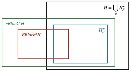
Figure 2. The relationship among $H,$ $H_F^{\pi },$$eBloc{k}^{\pi }H$ and $EBloc{k}^{\pi }H$ classes for the same partition $\pi .$

Let us emphasize that the choice of partition $\pi$ is usually defined by the problem itself, for example, according to the structure of the matrix observed.

Remark 7.

The computation complexity analysis of using $e{\mathrm{Block}}^{\pi }H$, $E{\mathrm{Block}}^{\pi }H$ and $H_F^{\pi }$ classes can be investigated by comparing the CPU times needed for the calculation of comparison matrices underlying them. For the purpose of the numerical experiment, a random dense matrix was constructed in MATLAB^® (version $R2024a$) on a workstation equipped with an Apple M4 Pro processor (14 cores), 24 GB of Unified Memory and running MacOS 15.6.1, taking $A=randn\left(n\right)+n*eye\left(n\right)$ with size $n=6561$ and different numbers of blocks $\mathsf{\ell },$ each partitioning the index set into ℓ subsets of equal length. After 50 runs for each $\mathsf{\ell },$ the average times (in seconds) were calculated with reports summarized in Table 1, and a plot comparing the number of blocks versus the runtime is provided in Figure 3.

Table 1. Summary of the numerical experiment taking the average CPU time for the computation of comparison matrices for 50 runs per each choice of $\mathsf{\ell }.$

ℓ	${\mathit{CPU}}_{\mathit{time}}$$(⟩\mathit{A}{⟨}_2^{\mathit{\pi }})$	${\mathit{CPU}}_{\mathit{time}}$$\left({⟨\mathit{A}⟩}_2^{\mathit{\pi }}\right)$	${\mathit{CPU}}_{\mathit{time}}$$\left({\mathit{A}}_{\mathit{F}}^{\mathit{\pi }}\right)$
27	7.4433	3.9727	1.3812
81	10.3618	4.2256	1.3980
243	26.4014	4.8978	1.4200
729	65.1657	12.0393	1.5597
2187	151.9813	38.6268	2.9426

Table 1. Summary of the numerical experiment taking the average CPU time for the computation of comparison matrices for 50 runs per each choice of $\mathsf{\ell }.$

ℓ	${\mathit{CPU}}_{\mathit{time}}$$(⟩\mathit{A}{⟨}_2^{\mathit{\pi }})$	${\mathit{CPU}}_{\mathit{time}}$$\left({⟨\mathit{A}⟩}_2^{\mathit{\pi }}\right)$	${\mathit{CPU}}_{\mathit{time}}$$\left({\mathit{A}}_{\mathit{F}}^{\mathit{\pi }}\right)$
27	7.4433	3.9727	1.3812
81	10.3618	4.2256	1.3980
243	26.4014	4.8978	1.4200
729	65.1657	12.0393	1.5597
2187	151.9813	38.6268	2.9426

Figure 3. The plot of the number of blocks ℓ versus the average CPU runtime (in seconds) to compute the three comparison matrices, $A_F^{\pi }$—blue, ${⟨A⟩}_2^{\pi }$—yellow, and ${⟩A⟨}_2^{\pi }$—red line.

After the calculation of these three different comparison matrices (${⟩A⟨}_2^{\pi },$${⟨A⟩}_2^{\pi }$ and $A_F^{\pi }$), to confirm if a matrix belongs to $e{\mathrm{Block}}^{\pi }H$, $E{\mathrm{Block}}^{\pi }H$ and $H_F^{\pi },$ in practice always reduces to verifying whether the comparison matrix belongs to some subclass of M-matrices; hence, the workload for that part of the job for all three classes is essentially the same.

5. Applications

5.1. Modeling of Infectious Diseases

An epidemic model provides a mathematical framework for describing the dynamics of a population in response to the spread of a specific infectious disease (COVID-19, measles, influenza, standard cough, tuberculosis, smallpox, malaria—just to name a few). The primary objective of developing such models is to understand the overall impact of the disease on the population, to predict its progression and to identify effective strategies for mitigating or eliminating its effects. For a comprehensive overview on this matter, consult [24,25,26]. Here, we will recall the SVEIRS model, which is an extension of the classical SEIR (Susceptible–Exposed–Infectious–Recovered) epidemic model, designed to capture additional dynamics such as vaccination and waning immunity in order to evaluate optimal vaccination strategies and disease persistence. In this formulation, the total population is divided into five epidemiological compartments: susceptible (S), vaccinated (V), exposed (E), infectious (I), and recovered (R) individuals. Transitions between these compartments capture key biological and public health mechanisms: susceptible individuals may become vaccinated or exposed through infection; exposed individuals progress to the infectious stage after a latent period; infectious individuals recover and acquire temporary immunity; and both vaccinated and recovered individuals may lose immunity and return to the susceptible class [24,26], as shown in Figure 4. In some formulations, demographic processes such as births and deaths are also included to account for long-term dynamics.

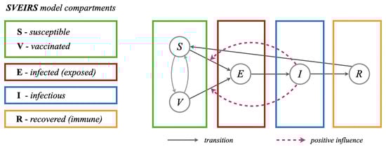
Figure 4. Schematic representation of interactions between model compartments in the SVEIRS epidemic model. Directional transitions between groups are marked with full arrows, where the dashed arrows represent a possible positive influence.

The fundamental role in analyzing the dynamical properties of this and other kinds of models from epidemiology belongs to the Jacobian matrix, which is obtained after linearization around the system steady states (equilibrium points). One of many such examples can be found in [26], where the author addressed the asymptotic stability of the disease-free equilibrium point (a steady state which eliminates the disease from the population) in the SVEIRS epidemic model with regular constant immunization (vaccination). The local asymptotic stability of this model is related to the Jacobian matrix $\overline{A^{*}}(\lambda ,\omega ),$ which has the following form:

$$\overline{A^{*}}(\lambda ,\omega ):=\left[\begin{array}{ccccc}(1-V_c)\nu -b& (1-V_c)\nu & (1-V_c)\nu & (1-V_c)\nu -{\displaystyle \frac{\beta S^{*}}{1+\eta S^{*}}}+\gamma e^{-b\omega }& (1-V_c)\nu \\ \nu V_c& \nu -(b+{\gamma }_1)& \nu V_c& \nu V_c-{\displaystyle \frac{\delta \beta V^{*}}{1+\eta V^{*}}}& \nu V_c\\ 0& 0& -b& \beta (1-e^{-b\omega })\left({\displaystyle \frac{S^{*}}{1+\eta S^{*}}}+{\displaystyle \frac{\delta V^{*}}{1+\eta V^{*}}}\right)& 0\\ 0& 0& 0& \beta e^{-b\lambda \omega }\left({\displaystyle \frac{S^{*}}{1+\eta S^{*}}}+{\displaystyle \frac{\delta V^{*}}{1+\eta V^{*}}}\right)-(\gamma +b+\alpha )& 0\\ 0& {\gamma }_1& 0& 1-\gamma e^{-b\omega }& -b\end{array}\right],$$

for more details, see [26]. Choosing the parameters of the epidemic model to be exactly the same as in [26], $\beta =0.0166 {\mathrm{days}}^{-1},$ $b=0.05 {\mathrm{days}}^{-1},$ $\nu =0.2b,$ $1/\alpha =1/\gamma =200 \mathrm{days},$ $1/{\gamma }_1=15 \mathrm{days},$ ${\beta }_1=\beta /2,$ $\delta ={\beta }_1/\beta ,$ $\tau =6 \mathrm{days},$ $\eta =0.5,$ $\omega =10 \mathrm{days},$ $\lambda =\tau /\omega =0.6,$ with $V_c=1$ for which $S^{*}=1,$ $V^{*}=0.107,$ $R^{*}=0.14,$ $I^{*}=E^{*}=0,$ we reconstructed the matrix:

$$A_4=\left[\begin{array}{ccccc}-0.05& 0& 0& -0.0302& 0\\ 0.01& -0.1067& 0.01& 0.0092& 0.01\\ 0& 0& -0.05& 0.0047& 0\\ 0& 0& 0& -0.0512& 0\\ 0& 0.0667& 0& 0.997& -0.05\end{array}\right].$$

Instead of calculating the eigenvalues, which is the (questionable) mainstream methodology (with a handful of potential computational drawbacks) used widely in this branch of applications, noting that the Jacobian matrix has negative diagonal entries by construction, we may employ our approach to investigate whether it is an H-matrix or not. We can see that the last row in $A_4$ disqualifies this matrix from being an $SDD$ one. More so, $\parallel D^{-1}{B\parallel }_F=19.9948>1;$ hence, it cannot be $SD{D}_F$. Also, this matrix is neither $S-SDD$ nor $S-SD{D}_F$ for any plausible nonempty proper subset $S.$ However, $A_4$ does belong to our new class $H_F^{\pi }$ for partitions: $\pi =\{0,1,2,4,5\}$ and $\pi =\{0,1,3,4,5\}.$ Then, according to Lemma 1, we can conclude that the system is locally stable, meaning that the infection will eventually be taken under control.

5.2. Ecological Modeling

Another significant real-life example we will use to illustrate the application potential of our new class of matrices rests on the grounds of the energetic food web framework [27], which represents a sophisticated mathematical model used to describe the complex network of interactions of living organisms in the soil food web and analyze how the flow of energy and nutrients shape the resilience and functioning of the network itself. Building upon these principles, the generalized Lotka–Volterra predator–prey model and its extensions [28,29] have been instrumental in demonstrating how interaction strengths and energy transfer pathways influence the stability of complex food webs. Together, these modeling approaches highlight the importance of energy-based and interaction-strength perspectives in understanding and predicting the behavior of real-world ecosystems.

The generalized Lotka–Volterra model assumes that species sharing similar food sources, feeding regimes, life span characteristics and habitats belong to the same functional group. At each functional group level, as well as among them, interactions that ensure the transfer of matter and the flow of energy through the system happen, which is illustrated in Figure 5.

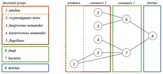
Figure 5. Schematic representation of interactions between functional groups in the energy flow of the soil food web systems in two possible configurations—three compartments system and an introduction of a fourth compartment via the separation of top predators.

The model assumes that the overall population N is subdivided into functional groups: $\mathcal{P}$ (primary producers), $\mathcal{C}$ (primary consumers) and $\mathcal{D}$ (detritivores). A special compartment, indexed with $n+1,$ is the pool of non-living organic matter (detritus). Taking into consideration the assimilation efficiency ${\left\{a_i\right\}}_{i=1}^{n+1},$ production efficiency ${\left\{p_i\right\}}_{i=1}^{n+1},$ the matrix of parameters of trophic interactions $C={\left\{c_{ij}\right\}}_{i,j=1}^{n+1}$ and the feasible equilibrium point (equilibrium biomass densities) ${\left\{x_i^{\star }\right\}}_{i=1}^{n+1},$ the Jacobian matrix $A=\left[{\alpha }_{ij}\right]$ is given by

$$\begin{array}{c}{\alpha }_{ij}=\left\{\begin{array}{cc}-c_{ii}{x}_i^{\star },& i=j,\\ -(c_{ij}-e_i{c}_{ji})x_i^{\star },& i\ne j,\end{array}\right. for i,j\in N\hfill \\ {\alpha }_{i,n+1}=\left\{\begin{array}{cc}0& i\in \mathcal{C}\cup \mathcal{P},\\ e_i{c}_{n+1,i}{x}_i^{\star },& i\in \mathcal{D},\end{array}\right.\hfill \\ \hfill \\ {\displaystyle {\alpha }_{n+1,j}=b_j-c_{n+1,j}{x}_{n+1}^{\star }+\sum _{k\in N\setminus \left\{j\right\}}(1-a_k)c_{jk}{x}_k^{\star },}\hfill \\ {\displaystyle {\alpha }_{n+1,n+1}=-\sum _{k\in N}{c}_{n+1,k}{x}_k^{\star }.}\hfill \end{array}$$

Since the main role in the stability analysis belongs to the Jacobian matrix calculated at the equilibrium point (the matrix also referred to as the community matrix), here we will only state a similar version of it, which is a strategy that was also used in [30]:

$$A_3=\left[\begin{array}{cccccccc}-6& 0& 0& 0& 0.02& 0.01& 0& 0\\ 0& -1.84& 0& 0& 0& 0.002& 0& 0\\ 0& 0& -1.92& 0& 0& 0.002& 0& 0\\ 0& 0& 0& -2.68& 0& 0.003& 0& 0\\ -0.026& 0& 0& 0& -6& 0.001& 0.01& 0\\ 0& -10.5& -13.65& -12.07& 0& -1.2& 0& 0.03\\ -15.76& 0& 0& 0& -15.76& 0& -1.2& 0.02\\ 0.5& 0.5& 0.5& 0.5& 0.5& -0.3& -0.3& -6\end{array}\right].$$

It is well known that all diagonal elements ${\alpha }_{ii}$ of the community matrix A are always negative. Moreover, their modulus quantifies intraspecific competition within the corresponding functional group (arising from competition for mates, food, space and similar resources). Also, the off-diagonal elements ${\alpha }_{ij}$ represent the mass-specific trophic interaction rates at the equilibrium. More accurately, the elements above the main diagonal of A represent the mass-specific predation rate of predator on its prey, while the mass-specific supply rates of prey to its predator are contained below the main diagonal. One can readily confirm that matrix $A_3$ belongs to our new class, more precisely, that it is an $H_F^{\pi }$-matrix and therefore an H-matrix as well. As a matter of fact, this is actually true for two distinct choices of partition: ${\pi }_1=\{0,5,7,8\}$ and ${\pi }_2=\{0,1,5,7,8\}.$ In practice, these partitions naturally correspond to the structural organization and hierarchy among functional group subpopulations in two possible configurations, where partition ${\pi }_2$ comes from ${\pi }_1$ by separating top predators and second-tier consumers in two detached groups. Also, matrix $A_3$ belongs to $E{\mathrm{Block}}^{\pi }H$-matrices for both of these partitions. However, from a practical point of view, this verification is computationally more demanding: it requires an inversion of appropriate ℓ diagonal blocks and the less favorable Euclidean matrix norm calculation (requiring eigenvalue computations).

As a conclusion, since $A_3$ has negative diagonal elements and belongs to the $H_F^{\pi }$ class, according to Lemma 1, the entire spectrum of $A_3$ lies in the open left-half complex plane, implying that the corresponding dynamical system is (locally) stable, meaning that the ecosystem will survive a small perturbation or external shock, achieving equilibrium eventually.

6. Comments on the Possible Approach via Other Norms

Instead of the Frobenius matrix norm, one could use some other matrix norms as well. Let ${\parallel ·\parallel }_{\left(m\right)}$ be an arbitrary consistent matrix norm. For any block matrix $A={\left[A_{ij}\right]}_{\mathsf{\ell }\times \mathsf{\ell }}$ of the form (2), whose diagonal entries are nonzero, we apply the same partition to $\left|J\right|=\left|J\right(A\left)\right|$ and define a special comparison matrix:

$$A_{\left(m\right)}^{\pi }=I-N_{\left(m\right)}\left(\right|J\left|\right).$$

Definition 2.

A matrix $A={\left[a_{ij}\right]}_{n\times n}$ of the block form (2) with nonzero diagonal entries is called an $H_{\left(m\right)}^{\pi }$-matrix if $A_{\left(m\right)}^{\pi }$ is a nonsingular M-matrix.

Now, we will prove the following theorem stating the nonsingularity property of an arbitrary $H_{\left(m\right)}^{\pi }$-matrix.

Theorem 2.

Every $H_{\left(m\right)}^{\pi }$-matrix is a nonsingular H-matrix.

Proof. 

Let A be an $H_{\left(m\right)}^{\pi }$-matrix, i.e., let $A_{\left(m\right)}^{\pi }$ be a nonsingular M-matrix, which means that $\rho \left(N_{\left(m\right)}\left(\left|J\right|\right)\right)<1.$ According to Lemma 2.4. from [31], it follows that

$$\rho \left(\left|J\right|\right)\le \rho \left(N_{\left(m\right)}\left(\right|J\left|\right)\right)<1,$$

which is sufficient for the comparison matrix $\mathcal{M}\left(A\right)$ to be a nonsingular M-matrix. Namely, $\mathcal{M}\left(A\right)=\left|D\right|-\left|B\right|$, and because of $\rho \left(\right|D{|}^{-1}\left|B\right|)<1$, we obtain

$$\begin{array}{cc}\hfill {\mathcal{M}\left(\mathcal{A}\right)}^{-1}& ={\left(\left|D\right|(I-|D{|}^{-1}\left|B\right|)\right)}^{-1}\hfill \\ & ={\left(I-{\left|D\right|}^{-1}\left|B\right|\right)}^{-1}{\left|D\right|}^{-1}\hfill \\ & =\sum _{k\ge 0}{\left({\left|D\right|}^{-1}\left|B\right|\right)}^k{\left|D\right|}^{-1}\ge 0,\hfill \end{array}$$

meaning that $\mathcal{M}\left(\mathcal{A}\right)$ is an M-matrix, i.e., A is a nonsingular H-matrix. □

Obviously, in the special case when ${\parallel ·\parallel }_{\left(m\right)}={\parallel ·\parallel }_{\infty }$ and $\pi =\{0,n\}$, our class coincides with the famous $SDD$ class, which is defined by

$${\parallel J\parallel }_{\infty }<1.$$

However, it seems more interesting to comment on the special case when ${\parallel ·\parallel }_{\left(m\right)}={\parallel ·\parallel }_{\infty }$ and $\pi =\{0,k,n\}$. Namely, our class is then defined by the condition

$$A_{\infty }^{\pi }=I-\left[\begin{array}{cc}\hfill \parallel J_{11}{\parallel }_{\infty }& \hfill \parallel J_{12}{\parallel }_{\infty }\\ \hfill \parallel J_{21}{\parallel }_{\infty }& \hfill \parallel J_{22}{\parallel }_{\infty }\end{array}\right] \mathrm{is}\mathrm{a}\mathrm{nonsingular}M-\mathrm{matrix}.$$

If we choose $S=\{1,2,\dots ,k\}$, where k is the dimension of $J_{11}$, the following theorem proves that our class is the subset of the $S-SDD$ class, which is defined by conditions (5) and (6).

Theorem 3.

If $A={\left[a_{ij}\right]}_{n\times n}$ of the block form (2), with nonzero diagonal entries, is an $H_{\infty }^{\pi }$-matrix, where $\pi =\{0,k,n\}$, then A is an $S-$SDD matrix for $S=\{1,2,\dots ,k\}$.

Proof. 

Let A be an $H_{\infty }^{\pi }$-matrix. Then, $A_{\infty }^{\pi }$ is a nonsingular M-matrix, and

$$\begin{array}{cc}\parallel J_{11}{\parallel }_{\infty }<1,\hfill & \hfill \hspace{1em}\hspace{1em}\hspace{1em}\hspace{1em}\hspace{1em}\hspace{1em}\hspace{1em}\hspace{1em}\hspace{1em}\hspace{1em}\end{array}$$

(11)

$$\left(1-\parallel J_{11}{\parallel }_{\infty }\right)\left(1-\parallel J_{22}{\parallel }_{\infty }\right)>\parallel J_{12}{\parallel }_{\infty }{\parallel J_{21}\parallel }_{\infty }.$$

(12)

Conditions (11) and (12) can be rewritten as

$$\underset{i\in S}{max}{\displaystyle \frac{r_i^S}{|a_{ii}|}}<1 and {\displaystyle \frac{{\displaystyle \underset{i\in S}{max}\frac{r_i^{\overline{S}}}{|a_{ii}|}}}{{\displaystyle 1-\underset{i\in S}{max}\frac{r_i^S}{|a_{ii}|}}}}·{\displaystyle \frac{{\displaystyle \underset{j\in \overline{S}}{max}\frac{r_j^S}{|a_{jj}|}}}{{\displaystyle 1-\underset{j\in \overline{S}}{max}\frac{r_j^{\overline{S}}}{|a_{jj}|}}}}<1,$$

from which it holds that

$$\underset{i\in S}{max}{\displaystyle \frac{r_i^S}{|a_{ii}|}}<1 and \underset{i\in S}{max}{\displaystyle \frac{\frac{r_i^{\overline{S}}}{|a_{ii}|}}{1-\frac{r_i^S}{|a_{ii}|}}}\underset{j\in \overline{S}}{max}{\displaystyle \frac{\frac{r_j^S}{|a_{jj}|}}{1-\frac{r_j^{\overline{S}}}{|a_{jj}|}}}<1,$$

which is equivalent with (5) and (6), meaning that A is an $S-$SDD matrix. □

7. Conclusions and Remarks

In this paper, we presented a new subclass of H-matrices that facilitates block necessity coming from the model itself and promotes the use of the Frobenius matrix norm. We emphasized the switch from the traditional, infinity-norm-based approach, which in real-life examples corresponds to individual magnitudes of interactions at every level, to the Frobenius norm, which highlights the aggregate interplay occurring within the system. The key novelty of our class is the increment in the number of blocks being considered, instead of two, as used in a recent publication. Apart from that, we have investigated the relationship of this new class of nonsingular matrices with respect to some well-known nonsingular block matrices based on the Euclidean matrix norm in order to underline that our new class is less computationally demanding when a matrix fits both classes. The computation complexity analysis of using both Euclidean and Frobenius norms is analyzed by comparing the CPU times needed for the calculation of corresponding comparison matrices. On random large dense matrices, the average CPU time grows more than 50 times if we use the Euclidean norm compared to the Frobenius one.

Numerical examples chosen for illustration come from the modeling of infectious diseases and ecological modeling with a clear application pathway in determining the local stability of such and similar continuous dynamical systems. Our new results presented in this paper could potentially offer a framework for the stability analysis of advanced variants of such dynamical systems housing more compartments and therefore encourage a possible future development and modernization of existing models in epidemiology. At present, these models predominantly depend on the explicit calculation of Jacobian eigenvalues and the subsequent calibration of model parameters that guarantee stability, which becomes a computational challenge as the dimensions of the system grow.

In this paper, we were guided by the existing matrix structure from the corresponding mathematical model, revealing the interconnections among interacting groups, and followed the block structure that has a realistic interpretation in the model. Certainly, the possibility and criteria for how to choose some other partitions, which are not directly implied by the structural composition of the complex model, which might provide a better answer, remains an open question.

References

- Fiedler, M.; Pták, V. On matrices with non-positive off-diagonal elements and positive principal minors. Czechoslov. Math. J. 1962, 12, 382–400. [Google Scholar] [CrossRef]
- Fiedler, M.; Pták, V. Generalized norms of matrices and the location of the spectrum. Czechoslov. Math. J. 1962, 12, 558–571. [Google Scholar] [CrossRef]
- Freingold, D.G.; Varga, R.S. Block diagonally dominant matrices and generalizations of the Gerschgorin circle theorem. Pac. J. Math. 1962, 12, 1241–1250. [Google Scholar] [CrossRef]
- Ostrowski, A.M. On Some Metrical Properties of Operator Matrices and Matrices Partitioned Into Blocks. J. Math. Anal. Appl. 1961, 2, 161–209. [Google Scholar] [CrossRef]
- Cvetković, D.L.; Cvetković, L.; Li, C.Q. CKV-type matrices with applications. Linear Algebra Appl. 2021, 608, 158–184. [Google Scholar] [CrossRef]
- Cvetković, L. H-matrix theory vs. eigenvalue localization. Numer. Algorithms 2006, 42, 229–245. [Google Scholar] [CrossRef]
- Cvetković, L.; Kostić, V.R.; Varga, R.S. A new Geršgorin-type eigenvalue inclusion set. Electron. Trans. Numer. Anal. 2004, 18, 73–80. Available online: https://etna.ricam.oeaw.ac.at/vol.18.2004/pp73-80.dir/pp73-80.pdf (accessed on 30 April 2004).
- Dashnic, L.S.; Zusmanovich, M.S. O nekotoryh kriteriyah regulyarnosti matric i lokalizacii ih spectra (Criteria for matrix regularity and spectrum localization). USSR Comput. Math. Math. Phys. 1970, 10, 1092–1097. [Google Scholar]
- Desplanques, J. Théorème d’Algébre. J. Mathématiques Spec. 1887, 9, 12–13. [Google Scholar]
- Doroslovački, K.; Cvetković, D.L. On matrices with only one non-SDD row. Mathematics 2023, 11, 2382. [Google Scholar] [CrossRef]
- Li, B.S.; Tsatsomeros, M.J. Doubly diagonally dominant matrices. Linear Algebra Appl. 1997, 261, 221–235. [Google Scholar] [CrossRef]
- Ostrowski, A.M. Über die Determinanten mit Überwiegender Hauptdiagonale (About the determinants with predominant main diagonal). Comment. Math. Helv. 1937, 10, 69–96. [Google Scholar] [CrossRef]
- Gao, Y.M.; Wang, X.H. Criteria for generalized diagonally dominant matrices and M-matrices. Linear Algebra Appl. 1992, 169, 257–268. [Google Scholar] [CrossRef]
- Pena, J.M. Diagonal dominance, Schur complements and some classes of H-matrices and P-matrices. Adv. Comput. Math. 2011, 35, 357–373. [Google Scholar] [CrossRef]
- Garcia-Esnaola, M.; Pena, J.M. Error bounds for the linear complementarity problem with a Σ − SDD matrix. Linear Algebra Appl. 2013, 438, 1339–1346. [Google Scholar] [CrossRef]
- Zhao, J.X.; Liu, Q.L.; Li, C.Q.; Li, Y.T. Dashnic-Zusmanovich type matrices: A new subclass of nonsingular H-matrices. Linear Algebra Appl. 2018, 552, 277–287. [Google Scholar] [CrossRef]
- Chen, X.; Li, Y.; Liu, L.; Wang, Y. Infinity norm upper bounds for the inverse of SDD1 matrices. AIMS Math. 2022, 7, 8847–8860. [Google Scholar] [CrossRef]
- Li, Y.; Wang, S. An Infinity Norm Upper Bound for the Inverse of SDD1 Matrices and the Application in Linear Complementarity Problems. Commun. Appl. Math. Comput. 2025. [Google Scholar] [CrossRef]
- Geng, Y.; Zhu, Y.; Zhang, F.; Wang, F. Infinity Norm Bounds for the Inverse of SDD1-Type Matrices with Applications. Commun. Appl. Math. Comput. 2025. [Google Scholar] [CrossRef]
- Cvetković, D.; Vukelić, Đ.; Doroslovački, K. A New Subclass of H-matrices with Applications. Mathematics 2024, 12, 2322. [Google Scholar] [CrossRef]
- Cvetković, L.; Kostić, V.R.; Doroslovački, K.; Cvetković, D.L. Euclidean norm estimates of the inverse of some special block matrices. Appl. Math. Comput. 2016, 284, 12–23. [Google Scholar] [CrossRef]
- Varga, R.S. Geršgorin and His Circles; Springer: New York, NY, USA, 2004; Available online: https://link.springer.com/book/10.1007/978-3-642-17798-9 (accessed on 11 August 2004).
- Robert, F. Blocs-H-matrices et convergence des methodes iteratives classiques par blocks. Linear Algebra Appl. 1969, 2, 223–265. [Google Scholar] [CrossRef]
- De la Sen, M.; Agarwal, R.P.; Ibeas, A.; Alonso-Quesada, S. On the Existence of Equilibrium Points, Boundedness, Oscillating Behavior and Positivity of a SVEIRS Epidemic Model under Constant and Impulsive Vaccination. Adv. Contin. Discrete Models 2011, 2011, 748608. [Google Scholar] [CrossRef]
- Anderson, R.M.; May, R.M. Infectious Diseases of Humans: Dynamics and Control; Oxford University Press: Oxford, UK, 1992. [Google Scholar] [CrossRef]
- Riobello, R.N. On Some New Mathematical Models for Infective Diseases: Analysis, Equilibrium, Positivity and Vaccination Controls. PhD Thesis, The Faculty of Science and Technology, University of Basque Country, Leioa, Spain, 2015. [Google Scholar]
- Moore, J.C.; de Ruiter, P.C. Energetic Food Webs—An Analysis of Real and Model Ecosystems; Oxford University Press: Oxford, UK, 2012; Available online: https://academic.oup.com/book/2389 (accessed on 31 May 2012).
- Neutel, A.M.; Heesterbeek, J.A.P.; van de Koppel, J.; Hoenderboom, G.; Vos, A.; Kaldeway, C.; Berendse, F.; de Ruiter, P.C. Reconciling complexity with stability in naturally assembling food webs (Letter). Nature 2007, 449, 599–602. [Google Scholar] [CrossRef] [PubMed]
- Neutel, P.C.; Thorne, M.A.S. Interaction strengths in balanced carbon cycles and the absence of a relation between ecosystem complexity and stability. Ecol. Lett. 2014, 17, 651–661. [Google Scholar] [CrossRef]
- Kostić, V.R.; Cvetković, L.; Cvetković, D.L. Pseudospectra localizations and their applications. Numer. Linear Algebra Appl. 2016, 23, 356–372. [Google Scholar] [CrossRef]
- Zhang, W.; Han, Z.-Z. Bounds for the spectral radius of block H-matrices. Electron. J. Linear Algebra 2006, 15, 269–273. Available online: https://journals.uwyo.edu/index.php/ela/article/view/399 (accessed on 1 January 2006). [CrossRef]
Disclaimer/Publisher’s Note: The statements, opinions and data contained in all publications are solely those of the individual author(s) and contributor(s) and not of MDPI and/or the editor(s). MDPI and/or the editor(s) disclaim responsibility for any injury to people or property resulting from any ideas, methods, instructions or products referred to in the content. |
© 2026 by the authors. Licensee MDPI, Basel, Switzerland. This article is an open access article distributed under the terms and conditions of the Creative Commons Attribution (CC BY) license.