Dynamic Behavior of a Delayed Model with One Core Enterprise and Four Satellite Enterprises

Abstract

In this paper, an economic competition–cooperation model is examined, which has one core enterprise and four satellite enterprises. This extends previous smaller models in the literature mathematically. The unique positive solution to the original solution after a change of variables corresponds to a trivial equilibrium of a linearized system. The instability of this linearized solution implies the instability of the positive solution to the original system. The instability of the positive solution and boundedness will force this system to have a periodic solution. Some sufficient conditions to guarantee the periodic oscillation of the solutions for this model are provided, and computer simulations are given to support the present criteria.

1. Introduction

Competition–cooperation is an important relationship in enterprise interactive models, especially in enterprise cluster systems. Clusters can foster a dynamic environment that encourages innovation through close relationships, information exchange, and a readily available pool of specialized talent and resources. It directly impacts their success, resilience, and contribution to regional economic development. In the last few decades, various competition–cooperation enterprises’ interactive models with or without time delays have been provided. For example, Liao et al. [1] proposed the following delayed differential equation model of the form

$$\left\{\begin{array}{c}{x}_1^{\prime }\left(t\right)=x_1\left(t\right)(r_1-a_1{x}_1(t-\tau )-b_1{(x_2(t-\tau )-c_2)}^2),\hfill \\ x_2^{\prime }\left(t\right)=x_2\left(t\right)(r_2-a_2{x}_2(t-\tau )+b_2{(x_1(t-\tau )-c_1)}^2),\hfill \\ x_1\left(t\right)=\psi \left(t\right),x_2\left(t\right)=\varphi \left(t\right),t\in [-\tau ,0].\hfill \end{array}\right.$$

(1)

where the variables $x_1\left(t\right)$ and $x_2\left(t\right)$ denote the output of two enterprises, respectively. $r_1$ and $r_2$ denote the intrinsic growth for the output of two enterprises, respectively. $c_1$ and $c_2$ denote the initial production of two enterprises, respectively. The effect of delay on the dynamical behavior of System (1) has been discussed. Zhang et al. [2] discussed a delayed competition and cooperation system relating to economic enterprise. The stability of the unique positive equilibrium and the existence of Hopf bifurcations were demonstrated by analyzing the associated characteristic equation. Muhammadhaji and Nureji [3] studied the competition and cooperation model of enterprises with variable coefficients as follows:

$$\left\{\begin{array}{c}{y}_1^{\prime }\left(t\right)=y_1\left(t\right)[c_1\left(t\right)-b_{11}\left(t\right)y_1(t-{\tau }_1)-b_{12}\left(t\right){(y_2(t-{\tau }_2)-d_2\left(t\right))}^2],\hfill \\ y_2^{\prime }\left(t\right)=y_2\left(t\right)[c_2\left(t\right)-b_{21}\left(t\right)y_2(t-{\tau }_2)-b_{22}\left(t\right){(y_1(t-{\tau }_1)-d_1\left(t\right))}^2].\hfill \end{array}\right.$$

(2)

A criterion on the periodic solution, extinction, permanence, and global attractiveness of the model was provided by employing the Lyapunov method and the comparison principle. Xu and Shao [4] discussed the periodic solution and global attractivity of model (2) with impulses. Muhammadhaji and Maimaiti [5] studied a non-autonomous competition and cooperation model of two enterprises with discrete feedback controls and constant delays. In [6], the authors considered the following model:

$$\left\{\begin{array}{c}{u}_1^{\prime }\left(t\right)=u_1\left(t\right)[r_1\left(t\right)-{\alpha }_1\left(t\right)u_1\left(t\right)-{\beta }_1\left(t\right){(u_2\left(t\right)-{\sigma }_2\left(t\right))}^2-a_1\left(t\right)v_1(t-{\eta }_1\left(t\right))],\hfill \\ v_1^{\prime }\left(t\right)=-{\delta }_1\left(t\right)v_1\left(t\right)+q_1\left(t\right)u_1(t-{\zeta }_1\left(t\right)),\hfill \\ u_2^{\prime }\left(t\right)=u_2\left(t\right)[r_2\left(t\right)-{\alpha }_2\left(t\right)u_2\left(t\right)-{\beta }_2\left(t\right){(u_1\left(t\right)-{\sigma }_1\left(t\right))}^2-a_2\left(t\right)v_2(t-{\eta }_2\left(t\right))],\hfill \\ v_2^{\prime }\left(t\right)=-{\delta }_2\left(t\right)v_2\left(t\right)+q_2\left(t\right)u_2(t-{\zeta }_2\left(t\right)).\hfill \end{array}\right.$$

(3)

Some new results on the competition and cooperation model of two enterprises with multiple delays and feedback controls were obtained. Lu et al. [7] dealt with a discrete competition model with multiple delays and feedback controls. Guerrini [8] discussed the effect of small delays in a competition and cooperation model of enterprises. Jiang et al. [9] investigated a class of coupled-group consensus problems of first-order and second-order agents under the influence of communication and input time delays. By utilizing cooperative and competitive interactions among agents, a novel consensus protocol was designed. Xu and Li [10] considered almost periodic solution problems for two enterprises with time-varying delays and feedback controls. In [11], by means of the comparison theorem of differential equations and the Lyapunov functional, the global asymptotical stability of a unique almost periodic solution for an enterprise cluster model was obtained. Peng et al. [12] discussed a class of enterprise cluster models with feedback controls and time-varying delays on time scales as follows:

$$\left\{\begin{array}{c}{u}_1^{▵}\left(t\right)=a_1\left(t\right)u_1\left(\sigma \left(t\right)\right)-u_2\left(t\right)[b_{11}\left(t\right)u_1\left(t\right)-{\tau }_1\left(t\right))+b_{12}\left(t\right)(u_2{(t-{\tau }_2\left(t\right)-c_2\left(t\right))}^2\hfill \\ +d_1\left(t\right)v_1(t-{\tau }_3\left(t\right))],\hfill \\ u_2^{▵}\left(t\right)=a_2\left(t\right)u_2\left(\sigma \left(t\right)\right)-u_2\left(t\right)[b_{21}\left(t\right)u_2\left(t\right)-{\tau }_4\left(t\right))+b_{22}\left(t\right)(u_1{(t-{\tau }_5\left(t\right)-c_2\left(t\right))}^2\hfill \\ +d_2\left(t\right)v_2(t-{\tau }_6\left(t\right))],\hfill \\ v_1^{▵}\left(t\right)=-{\alpha }_1\left(t\right)v_1\left(\sigma \left(t\right)\right)+e_1\left(t\right)v_1(t-{\tau }_7\left(t\right)),\hfill \\ v_2^{▵}\left(t\right)=-{\alpha }_2\left(t\right)v_2\left(\sigma \left(t\right)\right)+e_2\left(t\right)v_2(t-{\tau }_8\left(t\right)).\hfill \end{array}\right.$$

(4)

Based on the theory of periodic time scales and the fixed-point theorem of strict-set-contractions, some new sufficient conditions for the existence of positive periodic solutions of model (4) were obtained. Ren et al. [13,14] considered the convergence and prediction of output dynamics. Alfifi [15,16] investigated the stability and Hopf bifurcation of a model of competition and cooperation between two enterprises with reaction, diffusion, and delays. Muhammadhaji et al. [17] discussed dynamical behavior for a class of delayed competitive–mutualism systems. The authors in [18] studied the forced waves for diffusive competition systems in shifting environments. In [19], traveling wave solutions of a delayed cooperative system were discussed. For other properties of diffusive competition and cooperation systems, see [20,21,22,23]. In [24], the authors investigated the following competition–cooperation enterprise cluster model with one core enterprise and two satellite enterprises:

$$\left\{\begin{array}{c}{x}_1^{\prime }\left(t\right)=x_1\left(t\right)[r_1-a_1{x}_1\left(t\right)-b_1{x}_2\left(t\right)-c_1{(y(t-\tau )-d)}^2],\hfill \\ x_2^{\prime }\left(t\right)=x_2\left(t\right)[r_2-a_2{x}_2\left(t\right)-b_2{x}_1\left(t\right)-c_1{(y(t-\tau )-d)}^2],\hfill \\ y^{\prime }\left(t\right)=y\left(t\right)[r_3-a_{3}y\left(t\right)+c_2({(x_1(t-\tau )-d_1)}^2+{(x_2(t-\tau )-d_2)}^2].\hfill \end{array}\right.$$

(5)

The upper bound of both core enterprise output and satellite enterprise output were provided. By selecting $\tau$ as the bifurcating parameter, the conditions of local stability and Hopf bifurcation were discussed. However, in practice we know that a cluster system may be more than two satellite enterprises. One example of a core–satellite system might be an automobile manufacturer and four companies that supply different kinds of parts for the automobiles, such as electrical systems, computer software, transmissions, and brakes. Therefore, in this paper, we extend model (5) to the following competition–cooperation enterprise cluster model with one core enterprise, four satellite enterprises, and multiple delay systems:

$$\left\{\begin{array}{c}{x}_1^{\prime }\left(t\right)=x_1\left(t\right)[r_1-a_1{x}_1\left(t\right)-b_{12}{x}_2(t-{\tau }_2)-b_{13}{x}_3(t-{\tau }_3)-b_{14}{x}_4(t-{\tau }_4)\hfill \\ -c_1{(y(t-{\tau }_5)-d)}^2],\hfill \\ x_2^{\prime }\left(t\right)=x_2\left(t\right)[r_2-a_2{x}_2\left(t\right)-b_{23}{x}_3(t-{\tau }_3)-b_{24}{x}_4(t-{\tau }_4)-b_{21}{x}_1(t-{\tau }_1)\hfill \\ -c_2{(y(t-{\tau }_5)-d)}^2],\hfill \\ x_3^{\prime }\left(t\right)=x_3\left(t\right)[r_3-a_3{x}_3\left(t\right)-b_{34}{x}_4(t-{\tau }_4)-b_{31}{x}_1(t-{\tau }_1)-b_{32}{x}_2(t-{\tau }_2)\hfill \\ -c_3{(y(t-{\tau }_5)-d)}^2],\hfill \\ x_4^{\prime }\left(t\right)=x_4\left(t\right)[r_4-a_4{x}_4\left(t\right)-b_{41}{x}_1(t-{\tau }_1)-b_{42}{x}_2(t-{\tau }_2)-b_{43}{x}_3(t-{\tau }_3)\hfill \\ -c_4{(y(t-{\tau }_5)-d)}^2],\hfill \\ y^{\prime }\left(t\right)=y\left(t\right)[r_5-a_{5}y\left(t\right)+c_5{(x_1(t-{\tau }_1)-d_1)}^2+c_6{(x_2(t-{\tau }_2)-d_2)}^2\hfill \\ +c_7{(x_3(t-{\tau }_3)-d_3)}^2+c_8{(x_4(t-{\tau }_4)-d_4)}^2],\hfill \\ x_i\left(t\right)={\varphi }_i\left(t\right),y\left(t\right)=\psi \left(t\right),t\in [-max\{{\tau }_1,\cdots ,{\tau }_5\},0],\hfill \end{array}\right.$$

(6)

where all the parameter values are positive real numbers. $x_i\left(t\right),y\left(t\right)(i=1,\cdots ,4)$ are the outputs of satellite enterprises and the core enterprise, respectively; $r_i(i=1,\cdots ,5)$ are the intrinsic growth rates; $a_i(i=1,\cdots ,5)$ are the self-regulations of enterprises; $b_{ij}(i,j=1,\cdots ,4)$ are the competition rates between satellite enterprises $A_{x_i}$ and $A_{x_j}$; $c_i(i=1,\cdots ,4)$ are the competition rates between satellite enterprises and the core enterprise; $c_i(i=5,\cdots ,8)$ are the rates of conversion of commodity into the reproduction of enterprises; $d_i(i=1,\cdots ,4)$ are initial outputs of satellite enterprises; and d is the initial output of the core enterprise. Our aim is to investigate the periodic oscillation of System (6). We believe that one can use a general bifurcating method to discuss the existence of a bifurcating periodic solution in this system, as the authors conducted in [24]. However, it is worth establishing that the bifurcating method cannot easily determine the existence of a bifurcation periodic solution if time delays are different real numbers, as in our computer simulation. In this paper, we shall use the method of mathematical analysis to study the existence of oscillatory solutions of System (6).

2. Preliminaries

Obviously, ${(0,0,0,0,0)}^T$ is a trivial equilibrium point of System (6). However, we may address the non-trivial positive equilibrium point. Since $r_i(i=1,\cdots ,5)$ are positive real numbers, there exists a positive equilibrium point of System (6), say ${(x_1^{*},x_2^{*},x_3^{*},x_4^{*},y^{*})}^T$. Then, a change of variables $x_i\left(t\right)\to x_i\left(t\right)-x_i^{*},y\left(t\right)\to y\left(t\right)-y^{*},(i=1,2,\cdots ,4)$ can be performed, noting that

$$\left\{\begin{array}{c}{r}_1-2a_1{x}_1^{*}-b_{12}{x}_2^{*}-b_{13}{x}_3^{*}-b_{14}{x}_4^{*}-c_1{(y^{*}-d)}^2=0,\hfill \\ r_2-2a_2{x}_2^{*}-b_{23}{x}_3^{*}-b_{24}{x}_4^{*}-b_{21}{x}_1^{*}-c_2{(y^{*}-d)}^2=0,\hfill \\ r_3-2a_3{x}_3^{*}-b_{34}{x}_4^{*}-b_{31}{x}_1^{*}-b_{32}{x}_2^{*}-c_3{(y^{*}-d)}^2=0,\hfill \\ r_4-2a_4{x}_4^{*}-b_{41}{x}_1^{*}-b_{42}{x}_2^{*}-b_{43}{x}_3^{*}-c_4{(y^{*}-d)}^2=0,\hfill \\ r_5-2a_5{y}^{*}+c_5{(x_1^{*}-d_1)}^2+c_6{(x_2^{*}-d_2)}^2+c_7{(x_3^{*}-d_3)}^2+c_8{(x_4^{*}-d_4)}^2=0,\hfill \end{array}\right.$$

(7)

We have the following system (the details are in the Appendix A):

$$\left\{\begin{array}{c}{x}_1^{\prime }\left(t\right)=(r_1-2a_1{x}_1^{*}-b_{12}{x}_2^{*}-b_{13}{x}_3^{*}-b_{14}{x}_4^{*}-c_1{(y^{*}-d)}^2)x_1\left(t\right)-b_{12}{x}_1^{*}{x}_2(t-{\tau }_2)\hfill \\ -b_{13}{x}_1^{*}{x}_3(t-{\tau }_3)-b_{14}{x}_1^{*}{x}_4(t-{\tau }_4)-2c_1{x}_1^{*}(y^{*}-d)y(t-{\tau }_5)-a_1{x}_1^2\left(t\right)\hfill \\ -b_{12}{x}_1\left(t\right)x_2(t-{\tau }_2)-b_{13}{x}_1\left(t\right)x_3(t-{\tau }_3)-b_{14}{x}_1\left(t\right)x_4(t-{\tau }_4)-c_1{x}_1\left(t\right)y^2(t-{\tau }_5),\hfill \\ x_2^{\prime }\left(t\right)=(r_2-2a_2{x}_2^{*}-b_{23}{x}_3^{*}-b_{24}{x}_4^{*}-b_{21}{x}_1^{*}-c_2{(y^{*}-d)}^2)x_2\left(t\right)-b_{23}{x}_2^{*}{x}_3(t-{\tau }_3)\hfill \\ -b_{24}{x}_2^{*}{x}_4(t-{\tau }_4)-b_{21}{x}_2\left(t\right)x_1(t-{\tau }_1)-2c_2{x}_2^{*}(y^{*}-d)y(t-{\tau }_5)-a_2{x}_2^2\left(t\right)\hfill \\ -b_{23}{x}_2\left(t\right)x_3(t-{\tau }_3)-b_{24}{x}_2\left(t\right)x_4(t-{\tau }_4)-b_{21}{x}_2\left(t\right)x_1(t-{\tau }_1)-c_2{x}_2\left(t\right)y^2(t-{\tau }_5),\hfill \\ x_3^{\prime }\left(t\right)=(r_3-2a_3{x}_3^{*}-b_{34}{x}_4^{*}-b_{31}{x}_1^{*}-b_{32}{x}_2^{*}-c_3{(y^{*}-d)}^2)x_3\left(t\right)-b_{34}{x}_3^{*}{x}_4(t-{\tau }_4)\hfill \\ -b_{31}{x}_3^{*}{x}_1(t-{\tau }_1)-b_{32}{x}_3^{*}{x}_2(t-{\tau }_2)-2c_3{x}_3^{*}(y^{*}-d)y(t-{\tau }_5)-a_3{x}_3^2\left(t\right)\hfill \\ -b_{34}{x}_3\left(t\right)x_4(t-{\tau }_4)-b_{31}{x}_3\left(t\right)x_1(t-{\tau }_1)-b_{32}{x}_3\left(t\right)x_2(t-{\tau }_2)-c_3{x}_3\left(t\right)y^2(t-{\tau }_5),\hfill \\ x_4^{\prime }\left(t\right)=(r_4-2a_4{x}_4^{*}-b_{41}{x}_1^{*}-b_{42}{x}_2^{*}-b_{43}{x}_3^{*}-c_4{(y^{*}-d)}^2)x_4\left(t\right)-b_{41}{x}_4^{*}{x}_1(t-{\tau }_1)\hfill \\ -b_{42}{x}_4^{*}{x}_2(t-{\tau }_2)-b_{43}{x}_4^{*}\left(t\right)x_3(t-{\tau }_3)-2c_4{x}_4^{*}(y^{*}-d)y(t-{\tau }_5)-a_4{x}_4^2\left(t\right)\hfill \\ -b_{41}{x}_4\left(t\right)x_1(t-{\tau }_1)-b_{42}{x}_4\left(t\right)x_2(t-{\tau }_2)-b_{43}{x}_4\left(t\right)x_3(t-{\tau }_3)-c_4{x}_4\left(t\right)y^2(t-{\tau }_5),\hfill \\ y^{\prime }\left(t\right)=(r_5-2a_5{y}^{*}+c_5{y}^{*}{(x_1^{*}-d_1)}^2+c_6{y}^{*}{(x_2^{*}-d_2)}^2+c_7{y}^{*}{(x_3^{*}-d_3)}^2+c_8{y}^{*}{(x_4^{*}-d_4)}^2)y\left(t\right)\hfill \\ +2c_5{y}^{*}(x_1^{*}-d_1)x_1(t-{\tau }_1)+2c_6{y}^{*}(x_2^{*}-d_2)x_2(t-{\tau }_2)+2c_7{y}^{*}(x_3^{*}-d_3)x_3(t-{\tau }_3)\hfill \\ +2c_8{y}^{*}(x_4^{*}-d_4)x_4(t-{\tau }_4)-a_5{y}^2\left(t\right)+c_{5}y\left(t\right)x_1^2(t-{\tau }_1)+c_{6}y\left(t\right)x_2^2(t-{\tau }_2)\hfill \\ +c_{7}y\left(t\right)x_3^2(t-{\tau }_3)+c_{8}y\left(t\right)x_4^2(t-{\tau }_4).\hfill \end{array}\right.$$

(8)

System (8) can be expressed in the following matrix form:

$$\begin{array}{c}\hfill u^{\prime }\left(t\right)=Pu\left(t\right)+Qu(t-\tau )+f(u\left(t\right),u(t-\tau )),\end{array}$$

(9)

where $u\left(t\right)={[x_1\left(t\right),x_2\left(t\right),x_3\left(t\right),x_4\left(t\right),y\left(t\right)]}^T$, $u(t-\tau )=[x_1(t-{\tau }_1),x_2(t-{\tau }_2),x_3(t-{\tau }_3)$, $x_4(t-{\tau }_4),y(t-{\tau }_5){]}^T$, P and Q both are $5\times 5$ matrices, and $f\left(u\right(t), u(t-\tau \left)\right)$ is a five by one vector: $f(u\left(t\right),u(t-\tau ))=[-a_1{x}_1^2\left(t\right)-b_{12}{x}_1\left(t\right)x_2(t-{\tau }_2)-\cdots -c_1{x}_1\left(t\right)y^2(t-{\tau }_5)$, $\cdots -a_5{y}^2\left(t\right)+c_{5}y\left(t\right)x_1^2(t-{\tau }_1)+\cdots +c_{8}y\left(t\right)x_4^2(t-{\tau }_4){]}^T,$

$$\begin{array}{c}\hfill P=diag(a_{11},a_{22},a_{33},a_{44},a_{55}),\end{array}$$

where $a_{11}=r_1-2a_1{x}_1^{*}-b_{12}{x}_2^{*}-b_{13}{x}_3^{*}-b_{14}{x}_4^{*}-c_1{(y^{*}-d)}^2$, $a_{22}=r_2-2a_2{x}_2^{*}-b_{23}{x}_3^{*}-b_{24}{x}_4^{*}-b_{21}{x}_1^{*}-c_2{(y^{*}-d)}^2$, $a_{33}=r_3-2a_3{x}_3^{*}-b_{34}{x}_4^{*}-b_{31}{x}_1^{*}-b_{32}{x}_2^{*}-c_3{(y^{*}-d)}^2$, $a_{44}=r_4-2a_4{x}_4^{*}-b_{41}{x}_1^{*}-b_{42}{x}_2^{*}-b_{43}{x}_3^{*}-c_4{(y^{*}-d)}^2$, $a_{55}=r_5-2a_5{y}^{*}+c_5{y}^{*}{(x_1^{*}-d_1)}^2+c_6{y}^{*}{(x_2^{*}-d_2)}^2+c_7{y}^{*}{(x_3^{*}-d_3)}^2+c_8{y}^{*}{(x_4^{*}-d_4)}^2.$

$$\begin{array}{c}\hfill B={\left(b_{ij}\right)}_{5\times 5}=\left(\begin{array}{ccccc}0& q_{12}& q_{13}& q_{14}& q_{15}\\ q_{21}& 0& q_{23}& q_{24}& q_{25}\\ q_{31}& q_{32}& 0& q_{34}& q_{35}\\ q_{41}& q_{42}& q_{43}& 0& q_{45}\\ q_{51}& q_{52}& q_{53}& q_{54}& 0\end{array}\right),\end{array}$$

where $q_{12}=-b_{12}{x}_1^{*}$, $q_{13}=-b_{13}{x}_1^{*}$, $q_{14}=-b_{14}{x}_1^{*}$, $q_{15}=-2c_1{x}_1^{*}(y^{*}-d)$, $q_{21}=-b_{21}{x}_2^{*}$, $q_{23}=-b_{23}{x}_2^{*}$, $q_{24}=-b_{24}{x}_2^{*}$, $q_{25}=-2c_2{x}_2^{*}(y^{*}-d)$, $q_{31}=-b_{31}{x}_3^{*}$, $q_{32}=-b_{32}{x}_3^{*}$, $q_{34}=-b_{34}{x}_3^{*}$, $q_{35}=-2c_3{x}_3^{*}(y^{*}-d)$, $q_{41}=-b_{41}{x}_4^{*}$, $q_{42}=-b_{42}{x}_4^{*}$, $q_{43}=-b_{43}{x}_4^{*}$, $q_{45}=-2c_4{x}_4^{*}(y^{*}-d)$, $q_{51}=2c_5{y}^{*}(x_1^{*}-d_1)$, $q_{52}=2c_6{y}^{*}(x_2^{*}-d_2)$, $q_{53}=2c_7{y}^{*}(x_3^{*}-d_3)$, $q_{54}=2c_8{y}^{*}(x_4^{*}-d_4).$ The linearized equation of (9) is

$$\begin{array}{c}\hfill u^{\prime }\left(t\right)=Pu\left(t\right)+Qu(t-\tau )\end{array}$$

(10)

Lemma 1.

If matrix $N=P+Q$ is a nonsingular matrix for selected parameters, then there exists a unique positive equilibrium point for System (6).

Proof. 

To prove that there exists a unique positive equilibrium point for System (6), we only need to prove that Equation (10) has a unique trivial equilibrium point. Assume that $u^{*}={(x_1^{*},x_2^{*},x_3^{*},x_4^{*},y^{*})}^T$ is an equilibrium point of Equation (10); then, we have the following algebraic equations:

$$\begin{array}{c}\hfill (P+Q)u^{*}=N{u}^{*}=\mathbf{0}\end{array}$$

(11)

According to the basic linear algebraic knowledge, Equation (11) has a unique solution since $N=P+Q$ is a nonsingular matrix. This unique solution is exactly the trivial solution. This trivial solution of Equation (10) corresponds to the unique positive equilibrium point. In other words, System (6) has a unique positive equilibrium point. □

Remark 1.

Matrix $N=P+Q$ is a nonsingular matrix, which means that any two rows in matrix N are linearly independent. In other words, the parameter values of any two rows are not proportional.

Lemma 2.

All solutions of System (6) are bounded.

Proof. 

Note that all parameter values are positive real numbers in System (6). Thus, we have

$$\left\{\begin{array}{c}{x}_1^{\prime }\left(t\right)\le x_1\left(t\right)[r_1-a_1{x}_1\left(t\right)-b_{12}{x}_2(t-{\tau }_2)-b_{13}{x}_3(t-{\tau }_3)-b_{14}{x}_4(t-{\tau }_4)],\hfill \\ x_2^{\prime }\left(t\right)\le x_2\left(t\right)[r_2-a_2{x}_2\left(t\right)-b_{23}{x}_3(t-{\tau }_3)-b_{24}{x}_4(t-{\tau }_4)-b_{21}{x}_1(t-{\tau }_1)],\hfill \\ x_3^{\prime }\left(t\right)\le x_3\left(t\right)[r_3-a_3{x}_3\left(t\right)-b_{34}{x}_4(t-{\tau }_4)-b_{31}{x}_1(t-{\tau }_1)-b_{32}{x}_2(t-{\tau }_2)],\hfill \\ x_4^{\prime }\left(t\right)\le x_4\left(t\right)[r_4-a_4{x}_4\left(t\right)-b_{41}{x}_1(t-{\tau }_1)-b_{42}{x}_2(t-{\tau }_2)-b_{43}{x}_3(t-{\tau }_3)],\hfill \end{array}\right.$$

(12)

To prove the boundedness of the positive solutions in System (12), consider a Lyapunov function $V\left(t\right)={\displaystyle \frac{1}{2}}{\sum }_{i=1}^4{x}_i^2\left(t\right)$. Then, we get

$$\begin{array}{ccc}\hfill V^{\prime }{\left(t\right)|}_{\left(12\right)}& =& \sum _{i=1}^4{x}_i\left(t\right)x_i^{\prime }\left(t\right)\hfill \\ \hfill & \le & -\sum _{i=1}^4{a}_i{x}_i^3\left(t\right)-\sum _{i=1}^4\sum _{j=1,j\ne i}^4{b}_{ij}{x}_i^2\left(t\right)x_j(t-{\tau }_j)+\sum _{i=1}^4{r}_i{x}_i^2\left(t\right)\hfill \end{array}$$

(13)

Note that when $x_i\to +\infty ,$$x_i^3\left(t\right),x_i^2\left(t\right)x_j(t-{\tau }_j)$ are higher order infinite than $x_i^2\left(t\right)(i=1,\cdots ,4)$ since $a_i>0(i=1,\cdots ,4).$ Therefore, there exists suitably large $L>0$ such that $V^{\prime }{\left(t\right)|}_{\left(12\right)}<0$ as $x_i\left(t\right)>L(i=1,\cdots ,4)$. This means that $x_i\left(t\right)$ are bounded, say $x_i\left(t\right)\le K_i(i=1,\cdots ,4)$. From System (6), we have

$$\begin{array}{c}\hfill y^{\prime }\left(t\right)\le (r_5+c_5{K}_5^2+c_6{K}_6^2+c_7{K}_7^2+c_8{K}_8^2)y\left(t\right)-a_5{y}^2\left(t\right)\end{array}$$

(14)

Equation (14) is a Bernoulli equation (n = 2). Therefore, the solutions of $y\left(t\right)$ are bounded. Thus, all solutions of System (6) are bounded. □

3. The Existence of Periodic Oscillatory Solutions

Theorem 1.

Assume that System (6) has a unique positive equilibrium point. Let ${\rho }_1,{\rho }_2,\cdots ,{\rho }_5$ be characteristic values of matrix Q. If there is some $i\in \{1,\cdots ,5\}$, such that $Re\left({\rho }_i\right)>\left|a_{ii}\right|,$ then the unique positive equilibrium point of System (6) is unstable, implying that there exists an oscillatory solution in System (6).

Proof. 

Note that the nonlinear term $f\left(u\right(t),u(t-\tau \left)\right)$ of Equation (9) is a higher order infinitesimal as $u_i\to u_i^{*}.$ Obviously, if the trivial solution of Equation (10) is unstable, then the trivial solution of Equation (9) is unstable, implying that the unique positive equilibrium point of System (6) is unstable. Therefore, to discuss the instability of the positive equilibrium point of System (6), we only need to deal with the instability of the trivial solution of Equation (10). Since ${\rho }_1,{\rho }_2,\cdots ,{\rho }_5$ are characteristic values of matrix Q, then the characteristic equations associated with Equation (10) are the following:

$$\begin{array}{c}\hfill {\Pi }_{i=1}^5(\lambda -a_{ii}-{\rho }_i{e}^{-\lambda {\tau }_i})=0.\end{array}$$

(15)

Thus, we are led to investigate the nature of the roots for the following equation

$$\begin{array}{c}\hfill \lambda -a_{ii}-{\rho }_i{e}^{-\lambda {\tau }_i}=0.\end{array}$$

(16)

Equation (16) is a transcendental equation and it is hard to find all solutions for this equation. However, we show that there exists a positive real-part eigenvalue of Equation (16) under the assumption of Theorem 1. Indeed, if $Re\left({\rho }_i\right)>\left|a_{ii}\right|,$ setting $\lambda ={\lambda }_1+i{\lambda }_2$, ${\rho }_i={\rho }_{i1}+i{\rho }_{i2}, {\lambda }_1=Re\left(\lambda \right), {\lambda }_2=Im\left(\lambda \right), {\rho }_{i1}=Re\left({\rho }_i\right), {\rho }_{i2}=Im\left({\rho }_i\right)$. Separating the real part and imaginary part of Equation (16), we get

$$\begin{array}{c}\hfill {\lambda }_1=a_{ii}+{\rho }_{i1}{e}^{-{\lambda }_1{\tau }_i}cos\left({\lambda }_2{\tau }_1\right)-{\rho }_{i2}{e}^{-{\lambda }_1{\tau }_i}sin\left({\lambda }_2{\tau }_i\right)\end{array}$$

(17)

We show that Equation (17) has a positive root. Let

$$\begin{array}{c}\hfill h\left({\lambda }_1\right)={\lambda }_1-a_{ii}-{\rho }_{i1}{e}^{-{\lambda }_1{\tau }_i}cos\left({\lambda }_2{\tau }_1\right)+{\rho }_{i2}{e}^{-{\lambda }_1{\tau }_i}sin\left({\lambda }_2{\tau }_i\right)\end{array}$$

(18)

Obviously, $h\left({\lambda }_1\right)$ is a continuous function of ${\lambda }_1$. Noting that ${\rho }_{i1}>\left|a_{ii}\right|$, then $h\left(0\right)=-a_{ii}-{\rho }_{i1}cos\left({\lambda }_2{\tau }_i\right)+{\rho }_{i2}sin\left({\lambda }_2{\tau }_i\right)\sim -a_{ii}-{\rho }_{i1}<0.$ as ${\lambda }_2{\tau }_i\sim 2n\pi$, where n is an integer number. Since ${lim}_{{\lambda }_1\to +\infty }{e}^{-{\lambda }_1{\tau }_i}=0$, there exists a suitably large ${\lambda }_1$, say ${\lambda }_1^{*}(>0)$ such that $h\left({\lambda }_1^{*}\right)={\lambda }_1^{*}-a_{ii}-{\rho }_{i1}{e}^{-{\lambda }_1^{*}{\tau }_i}cos\left({\lambda }_2{\tau }_i\right)+{\rho }_{i2}{e}^{-{\lambda }_1^{*}{\tau }_i}sin\left({\lambda }_2{\tau }_i\right)>0.$ By the Intermediate Value Theorem, there exists a ${\lambda }_1,$ say ${\lambda }_1^0\in (0,{\lambda }_1^{*})$, such that $h\left({\lambda }_1^0\right)=0,$ implying that there is a positive real-part characteristic value of Equation (16). This means that the trivial solution of Equation (10) is unstable, implying that the trivial solution of System (8) is unstable. Note that the trivial solution of System (8) corresponds to the unique positive equilibrium of System (6); this means that the unique positive equilibrium point ${(x_1^{*}, x_2^{*}, x_3^{*}, x_4^{*}, y^{*})}^T$ of System (6) is unstable. This instability of the unique positive equilibrium point, together with the boundedness of the solutions, will force System (6) to generate a limit circle, namely, there is a periodic oscillatory solution in System (6) [25,26]. The proof is completed. □

Now set $\alpha ={min}_{1\le i\le 5}|a_{ii}|, \overline{\alpha }={max}_{1\le i\le 5}|a_{ii}|, \beta ={max}_j{\sum }_{i=1,i\ne j}^5|q_{ij}|.$ Then, we have the following theorem.

Theorem 2.

Assume that the conditions of Lemma 1 and Lemma 2 hold. If for each $a_{ii}<0$$(i=1,\cdots ,5)$, the following inequality holds,

$$\begin{array}{c}\hfill -\alpha +\beta >0,\end{array}$$

(19)

or for each $a_{ii}>0(i=1,\cdots ,5),$

$$\begin{array}{c}\hfill \overline{\alpha }-\beta <0.\end{array}$$

(20)

then the unique positive equilibrium point of System (6) is unstable, implying that System (6) generates a periodic oscillatory solution.

Proof. 

Note that $|v(t)|=v\left(t\right)$ as $v\left(t\right)>0,$ and $|v(t)|=-v\left(t\right)$ as $v\left(t\right)<0.$ So, from (10), we have

$$\left\{\begin{array}{c}{\displaystyle \frac{d|x_1\left(t\right)|}{dt}}\le a_{11}|x_1\left(t\right)|+|b_{12}{x}_1^{*}||x_2(t-{\tau }_2)|+|b_{13}{x}_1^{*}||x_3(t-{\tau }_3)|\hfill \\ +|b_{14}{x}_1^{*}||x_4(t-{\tau }_4)|+|2c_1{x}_1^{*}(y^{*}-d)||y(t-{\tau }_5)|,\hfill \\ {\displaystyle \frac{d|x_2\left(t\right)|}{dt}}\le a_{22}|x_2\left(t\right)|+|b_{23}{x}_2^{*}||x_3(t-{\tau }_3)|+|b_{24}{x}_2^{*}||x_4(t-{\tau }_4)|\hfill \\ +|b_{21}{x}_2^{*}||x_1(t-{\tau }_1)|+|2c_2{x}_2^{*}(y^{*}-d)||y(t-{\tau }_5)|,\hfill \\ {\displaystyle \frac{d|x_3\left(t\right)|}{dt}}\le a_{33}|x_3\left(t\right)|+|b_{34}{x}_3^{*}||x_4(t-{\tau }_4)|+|b_{31}{x}_3^{*}||x_1(t-{\tau }_1)|\hfill \\ +|b_{32}{x}_3^{*}||x_2(t-{\tau }_2)|+|2c_3{x}_3^{*}(y^{*}-d)||y(t-{\tau }_5)|,\hfill \\ {\displaystyle \frac{d|x_4\left(t\right)|}{dt}}\le a_{44}|x_4\left(t\right)|+|b_{41}{x}_4^{*}||x_1(t-{\tau }_1)|+|b_{42}{x}_4^{*}||x_2(t-{\tau }_2)|\hfill \\ +|b_{43}{x}_4^{*}||x_3(t-{\tau }_3)|+|2c_4{x}_4^{*}(y^{*}-d)||y(t-{\tau }_5)|,\hfill \\ {\displaystyle \frac{d|y(t)|}{dt}}\le a_{55}|y\left(t\right)|+2|c_5{y}^{*}(x_1^{*}-d_1)||x_1(t-{\tau }_1)|+2|c_6{y}^{*}(x_2^{*}-d_2)||x_2(t-{\tau }_2)|\hfill \\ 2|c_7{y}^{*}(x_3^{*}-d_3)||x_3(t-{\tau }_3)|+2|c_8{y}^{*}(x_4^{*}-d_4)||x_4(t-{\tau }_4)|.\hfill \end{array}\right.$$

(21)

Let $z\left(t\right)={\sum }_{i=1}^4(|x_i\left(t\right)|+|y\left(t\right)|)$. Since $a_{ii}<0(i=1,\cdots ,5)$, from (19), we have

$$\begin{array}{c}\hfill {\displaystyle \frac{dz\left(t\right)}{dt}}\le -\alpha z\left(t\right)+\beta z(t-\tau )\end{array}$$

(22)

Consider a scalar delayed differential equation

$$\begin{array}{c}\hfill {\displaystyle \frac{dw\left(t\right)}{dt}}=-\alpha z\left(t\right)+\beta z(t-\tau )\end{array}$$

(23)

Obviously, we have $z\left(t\right)\le w\left(t\right).$ We prove that the trivial solution of Equation (23) is unstable. Indeed, the characteristic equation associated with Equation (23) is the following:

$$\begin{array}{c}\hfill \lambda =-\alpha +\beta e^{-\lambda \tau }\end{array}$$

(24)

Similar to Theorem 1, consider a function $g\left(\lambda \right)=\lambda +\alpha -\beta e^{-\lambda \tau }$. Then, $g\left(0\right)=\alpha -\beta <0$ since $-\alpha +\beta >0$. There exists a suitably large $\lambda$, say ${\lambda }_{*}(>0)$, such that $g\left({\lambda }_{*}\right)={\lambda }_{*}+\alpha -\beta e^{-{\lambda }_{*}\tau }>0.$ So there exists a $\lambda ,$ say ${\lambda }_0\in (0,{\lambda }_{*})$ such that $g\left({\lambda }_0\right)=0,$ implying that there is a positive real-part characteristic value of Equation (23). This means that the trivial solution of System (10) is unstable. It suggests that the unique positive equilibrium point ${(x_1^{*}, x_2^{*}, x_3^{*}, x_4^{*}, y^{*})}^T$ of System (6) is unstable, and System (6) has an oscillatory solution. In case (20), the proof is similar to (19), so we omit it. □

4. Simulation Result

This simulation is based on System (6). Firstly, the parameters are selected as follows: $r_1=0.88, r_2=0.86$, $r_3=0.82$, $r_4=0.84$, $r_5=0.87$, $a_1=0.78$, $a_2=0.76$, $a_3=0.74$, $a_4=0.78$, $a_5=0.75$, $b_{12}=0.41$, $b_{13}=0.35$, $b_{14}=0.46$, $b_{21}=0.36$, $b_{23}=0.38$, $b_{24}=0.26$, $b_{31}=0.34$, $b_{32}=0.47$, $b_{34}=0.42$, $b_{41}=0.28$, $b_{42}=0.32$, $b_{43}=0.32$, $c_1=0.042$, $c_2=0.032,$$c_3=0.025$, $c_4=0.024$, $c_5=3.75$, $c_6=3.90$, $c_7=3.85$, $c_8=3.75$, $d_1=0.125$, $d_2=0.128$, $d_3=0.122$, $d_4=0.124$, $d=0.12.$ Then, the unique positive equilibrium point is ${(0.1661,0.5959,0.1824,0.5038,2.4243)}^T.$ Therefore, matrix P = diag$(-0.1477,-0.4339,-0.1269,-0.3621,0.6472)$, $q_{12}=-0.0681, q_{13}=-0.0581$, $q_{14}=-0.0764$, $q_{15}=-0.1608, q_{21}=-0.2037, q_{23}=-0.2150,$$q_{24}=-0.1471$, $q_{25}=-0.0835$, $q_{31}=-0.0621$, $q_{32}=-0.0858$, $q_{34}=-0.0766$, $q_{35}=-0.0210$, $q_{41}=-0.1441$, $q_{42}=-0.1612$, $q_{43}=-0.1612$, $q_{45}=-0.0581$, $q_{51}=0.8775$, $q_{52}=8.2805$, $q_{53}=1.4227$, $q_{54}=8.7471.$ The characteristic values of matrix Q are $0.1571, -0.3399\pm 1.1649i, -0.2616\pm 0.3112i$. Noting that $0.1571>|-0.1269|$, the conditions of Theorem 1 are satisfied. When time delays are selected as ${\tau }_1=2.75, {\tau }_2=2.82, {\tau }_3=2.78, {\tau }_4=2.72, {\tau }_5=2.74,$ and ${\tau }_1=2.91, {\tau }_2=2.98, {\tau }_3=2.94, {\tau }_4=2.88, {\tau }_5=2.90$, respectively, there exists an oscillatory solution for System (6) (see Figure 1 and Figure 2).

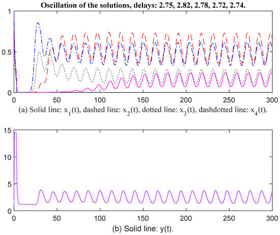
Figure 1. Oscillation of the solutions, delays: 2.75, 2.82, 2.78, 2.72, 2.74.

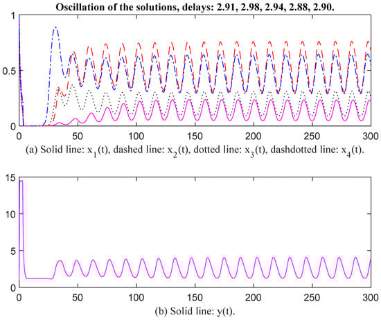
Figure 2. Oscillation of the solutions, delays: 2.91, 2.98, 2.94, 2.88, 2.90.

Then we select parameter values as $r_1=0.78$, $r_2=0.76$, $r_3=0.72$, $r_4=0.75$, $r_5=0.74$, $a_1=0.62$, $a_2=0.65$, $a_3=0.64$, $a_4=0.68$, $a_5=0.66$, $b_{12}=0.15$, $b_{13}=0.25$, $b_{14}=0.26$, $b_{21}=0.16$, $b_{23}=0.28$, $b_{24}=0.18$, $b_{31}=0.24$, $b_{32}=0.25$, $b_{34}=0.22$, $b_{41}=0.28$, $b_{42}=0.24$, $b_{43}=0.25$, $c_1=0.024$, $c_2=0.030,$$c_3=0.025$, $c_4=0.024$, $c_5=3.75$, $c_6=2.90$, $c_7=3.45$, $c_8=4.25$, $d_1=0.095$, $d_2=0.098$, $d_3=0.122$, $d_4=0.082$, $d=0.32.$ Then, the unique positive equilibrium point is ${(0.3516,0.4860,0.4093,0.3518,2.7475)}^T.$ The matrix P = diag$(-0.0653,-0.2284,-0.3569,0.0178,0.6432)$, $q_{12}=-0.0524$, $q_{13}=-0.0879$, $q_{14}=-0.0914$, $q_{15}=-0.0393$, $q_{21}=-0.0778$, $q_{23}=-0.1361,$$q_{24}=-0.0875$, $q_{25}=-0.0678$, $q_{31}=-0.0982$, $q_{32}=-0.1023$, $q_{34}=-0.0737$, $q_{35}=-0.1158$, $q_{41}=-0.0985$, $q_{42}=-0.0544$, $q_{43}=-0.0880$, $q_{45}=-0.0393$, $q_{51}=5.2843$, $q_{52}=6.2532$, $q_{53}=2.2584$, $q_{54}=6.2541.$ In this case, the characteristic values of matrix Q are $0.1801, 0.0948, 0.0482, -0.1615\pm 1.0676i$. Since $0.1801>|-0.0653|$, the conditions of Theorem 1 are satisfied. When time delays are selected as ${\tau }_1=3.54,{\tau }_2=3.70$, ${\tau }_3=3.65,{\tau }_4=3.50,{\tau }_5=3.52,$ and ${\tau }_1=4.04,{\tau }_2=4.20,{\tau }_3=4.15,{\tau }_4=4.00,{\tau }_5=4.02,$ respectively, there exists an oscillatory solution for System (6) (see Figure 3 and Figure 4). It seems that $x_1\left(t\right),x_2\left(t\right),x_3\left(t\right)$, and $x_4\left(t\right)$ have the same oscillatory frequency in Figure 3 and Figure 4. When time delays are increased, the oscillatory frequency is down slightly, which indicates that time delay affects the oscillatory frequency.

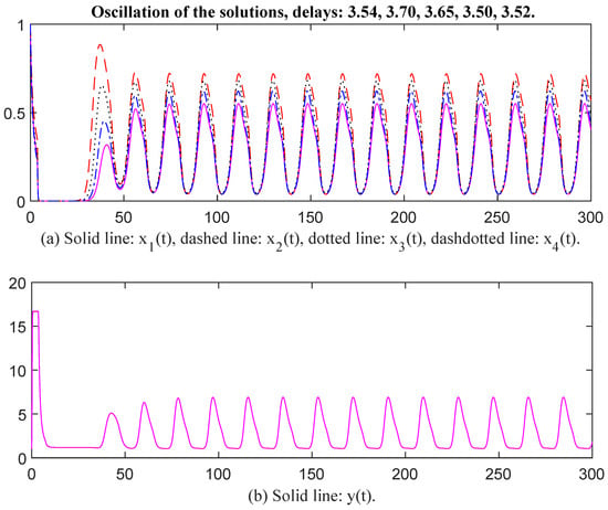
Figure 3. Oscillation of the solutions, delays: 3.54, 3.70, 3.65, 3.50, 3.52.

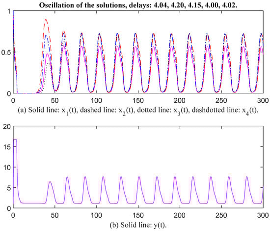
Figure 4. Oscillation of the solutions, delays: 4.04, 4.20, 4.15, 4.00, 4.02.

Then we select parameter values as $r_1=0.96$, $r_2=0.94$, $r_3=0.92$, $r_4=0.95$, $r_5=0.98$, $a_1=0.63$, $a_2=0.64$, $a_3=0.65$, $a_4=0.63$, $a_5=0.65$, $b_{12}=0.15$, $b_{13}=0.25$, $b_{14}=0.26$, $b_{21}=0.16$, $b_{23}=0.28$, $b_{24}=0.18$, $b_{31}=0.24$, $b_{32}=0.25$, $b_{34}=0.22$, $b_{41}=0.28$, $b_{42}=0.24$, $b_{43}=0.25$, $c_1=0.24$, $c_2=0.30$, $c_3=0.25$, $c_4=0.24$, $c_5=0.95$, $c_6=0.98$, $c_7=0.85$, $c_8=0.83$, $d_1=0.45$, $d_2=0.48$, $d_3=0.38$, $d_4=0.44$, $d=0.92.$ The unique positive equilibrium point is ${(0.7345,0.6182,0.4871,0.5093,1.7733)}^T.$ Therefore, matrix P = diag$(-0.1915,-0.2456,-0.1492,-0.1576,-1.3526)$, $q_{12}=-0.1102$, $q_{13}=-0.1836$, $q_{14}=-0.1912$, $q_{15}=-0.0312$, $q_{21}=-0.0978$, $q_{23}=-0.1731$, $q_{24}=-0.1137$, $q_{25}=-0.0315$, $q_{31}=-0.1176$, $q_{32}=-0.1225$, $q_{34}=-0.1078$, $q_{35}=-0.0209$, $q_{41}=-0.1432$, $q_{42}=-0.1205$, $q_{43}=-0.1273$, $q_{45}=-0.0208$, $q_{51}=1.0087$, $q_{52}=0.5067$, $q_{53}=0.5955$, $q_{54}=0.2146.$ The characteristic values of matrix Q are $0.0901, 0.1436, 0.1478, -0.1958\pm 0.1471i$. Obviously, the conditions of Theorem 1 are not satisfied. However, we see that $-\alpha =-0.1492, \beta =1.3675,$ and $-\alpha +\beta >0.$ The conditions of Theorem 2 are satisfied. This means that Theorem 1 is a stronger sufficient condition than that of Theorem 2. When time delays are selected as ${\tau }_1=4.04$, ${\tau }_2=4.20$, ${\tau }_3=4.15$, ${\tau }_4=4.00$, ${\tau }_5=4.02$, $d=0.92$ and ${\tau }_1=4.14, {\tau }_2=4.30, {\tau }_3=4.25, {\tau }_4=4.10, {\tau }_5=4.12,$$d=1.12$, respectively, there exists an oscillatory solution for System (6) (see Figure 5 and Figure 6). We see that the value of d affects oscillatory amplitude.

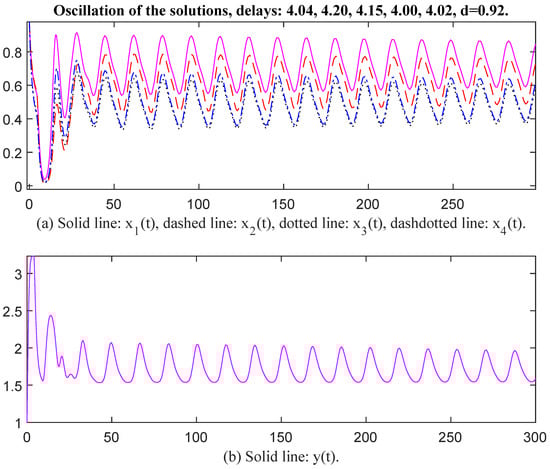
Figure 5. Oscillation of the solutions, delays: 4.04, 4.20, 4.15, 4.00, 4.02, d = 0.92.

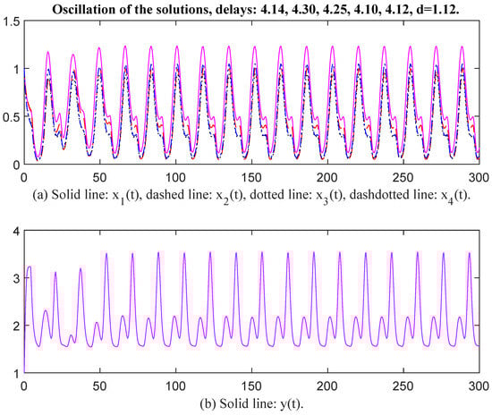
Figure 6. Oscillation of the solutions, delays: 4.14, 4.30, 4.25, 4.10, 4.12, d = 1.12.

In Figure 7 and Figure 8, the parameter values for $r_i, a_i$ and $c_i$ are selected the same as in Figure 5 and Figure 6, and the values $b_{ij}$ are changed to $b_{12}=0.015$, $b_{13}=0.025$, $b_{14}=0.026$, $b_{21}=0.016$, $b_{23}=0.028$, $b_{24}=0.018$, $b_{31}=0.024$, $b_{32}=0.025$, $b_{34}=0.022$, $b_{41}=0.028$, $b_{42}=0.024$, $b_{43}=0.025.$ When time delays are selected as ${\tau }_1=1.55$, ${\tau }_2=1.58$, ${\tau }_3=1.56$, ${\tau }_4=1.60$, ${\tau }_5=1.52,$ and ${\tau }_1=2.15$, ${\tau }_2=2.18$, ${\tau }_3=2.16$, ${\tau }_4=2.20$, ${\tau }_5=2.12,$ respectively, there exists an oscillatory solution for System (6). From Figure 7 and Figure 8, it is evident that the time delay affects the oscillatory frequency. Then the parameter values for $r_i, a_i, c_i$ and $b_{ij}$ are selected the same as in Figure 7 and Figure 8, except we change the values of $d_i$ to $d_1=0.35, d_2=0.38, d_3=0.28, d_4=0.34$. Then the unique positive equilibrium point is ${(0.5732, 0.2235, 0.4835, 0.5424, 2.0214)}^T.$ Therefore, matrix P = diag$(-0.3591, -0.1430, -0.3142, -0.3415, -1.3065)$, $q_{12}=-0.0086$, $q_{13}=-0.0143$, $q_{14}=-0.0145$, $q_{15}=-0.3496$, $q_{21}=-0.0036$, $q_{23}=-0.0063,$$q_{24}=-0.0039$, $q_{25}=-0.1699$, $q_{31}=-0.0115$, $q_{32}=-0.0121$, $q_{34}=-0.0108$, $q_{35}=-0.3051$, $q_{41}=-0.0148$, $q_{42}=-0.0142$, $q_{43}=-0.0148$, $q_{45}=-0.3295$, $q_{51}=0.8525$, $q_{52}=-0.6435$, $q_{53}=0.6438$, $q_{54}=0.6532.$ Thus, $-\alpha =-0.1430, \beta =1.1541,$ and $-\alpha +\beta >0.$ The conditions of Theorem 2 are satisfied. When time delays are selected as ${\tau }_1=1.55$, ${\tau }_2=1.58$, ${\tau }_3=1.56$, ${\tau }_4=1.60$, ${\tau }_5=1.52, d=1.25$ and ${\tau }_1=2.15$, ${\tau }_2=2.18$, ${\tau }_3=2.16$, ${\tau }_4=2.20$, ${\tau }_5=2.12$, $d=1.95$, respectively, there exists an oscillatory solution for System (6) (see Figure 9 and Figure 10). Again, the value of d affects oscillatory amplitude. The greater the value of d, the higher the oscillatory amplitude of the solution.

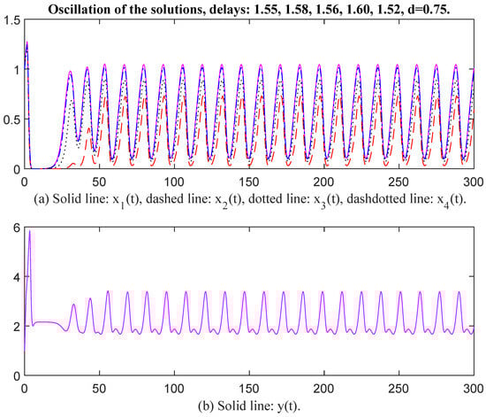
Figure 7. Oscillation of the solutions, delays: 1.55, 1.58, 1.56, 1.60, 1.52, d = 0.75.

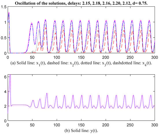
Figure 8. Oscillation of the solutions, delays: 2.15, 2.18, 2.16, 2.20, 2.12, d = 0.75.

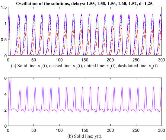
Figure 9. Oscillation of the solutions, delays: 1.55, 1.58, 1.56, 1.60, 1.52, d = 1.25.

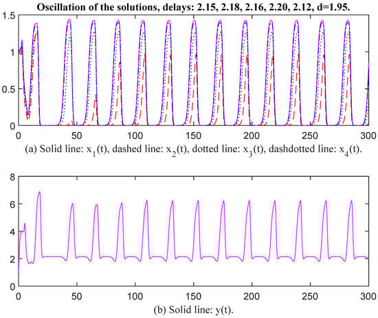
Figure 10. Oscillation of the solutions, delays: 2.15, 2.18, 2.16, 2.20, 2.12, d = 1.95.

Finally, we select the parameter values as $r_1=0.76$, $r_2=0.88$, $r_3=0.72$, $r_4=0.75$, $r_5=0.78$, $a_1=0.53$, $a_2=0.54$, $a_3=0.55$, $a_4=0.53$, $a_5=0.48,$$b_{12}=0.025$, $b_{13}=0.024$, $b_{14}=0.026$, $b_{21}=0.016$, $b_{23}=0.028$, $b_{24}=0.018$, $b_{31}=0.024$, $b_{32}=0.025$, $b_{34}=0.022$, $b_{41}=0.028$, $b_{42}=0.024$, $b_{43}=0.025$. $c_1=0.48$, $c_2=0.60$, $c_3=0.50$, $c_4=0.48$, $c_5=1.96$, $c_6=1.98$, $c_7=1.85$, $c_8=3.83$, $d_1=0.45$, $d_2=0.48$, $d_3=0.38$, $d_4=0.44$, d = 4.85. Then the unique positive equilibrium point is ${(0.2256, 0.1033, 0.0342, 0.1923, 4.1253)}^T.$ The matrix P = diag$(0.2586,0.4484,0.4041,0.2789,0.2578)$, $q_{12}=-0.0058$, $q_{13}=-0.0054$, $q_{14}=-0.0058$, $q_{15}=0.7267$, $q_{21}=-0.0004$, $q_{23}=-0.0029,$$q_{24}=-0.0004, q_{25}=0.0901$, $q_{31}=-0.0008$, $q_{32}=-0.0008$, $q_{34}=-0.0007$, $q_{35}=0.0241$, $q_{41}=-0.0054$, $q_{42}=-0.0046$, $q_{43}=-0.0048$, $q_{45}=0.1348$, $q_{51}=-3.5345$, $q_{52}=-3.0445$, $q_{53}=-2.6378$, $q_{54}=-7.8235.$ Therefore, $\alpha =0.4484, \beta =7.8304,$ and $\alpha -\beta <0.$ The conditions of Theorem 2 are satisfied. When time delays are selected as ${\tau }_1=0.75, {\tau }_2=0.78, {\tau }_3=0.76, {\tau }_4=0.80, {\tau }_5=0.72,$ and ${\tau }_1=1.15, {\tau }_2=1.18, {\tau }_3=1.16, {\tau }_4=1.20, {\tau }_5=1.12,$ respectively, there exists an oscillatory solution for System (6) (see Figure 11 and Figure 12). We see that the curves of $x_1\left(t\right), x_2\left(t\right), x_3\left(t\right)$ and $x_4\left(t\right)$ have the same oscillatory frequency, and the curves are jagged. Note that the characteristic values of matrix Q are $0.0092, 0.0011, 0.0005, -0.0054\pm 1.9902i$. The conditions of Theorem 1 are not satisfied, which means that Theorem 1 is a stronger sufficient condition again. From the above figures, we see that the values of $r_i$ are greater than those of the corresponding $a_i$ as an oscillation occurred, and the values of $c_i$ and $d_i$ must be restricted to within a limited interval. In other words, enterprises may possess a natural capacity for growth that outpaces their ability to establish and adhere to effective internal regulations. The rate at which raw materials or products are transformed into assets for reproduction or initial outputs of satellite enterprises is falling short of the inherent growth rate. Suppose enterprises fail to effectively convert commodities into reproductive assets and initial outputs for satellite enterprises, their ability to sustain growth and adapt to changing market conditions may be compromised in the long term.

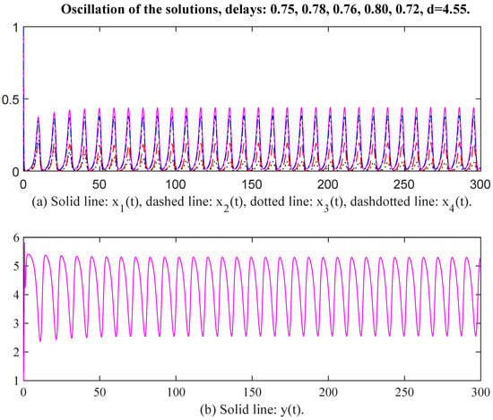
Figure 11. Oscillation of the solutions, delays: 0.75, 0.78, 0.76, 0.80, 0.72, d = 4.55.

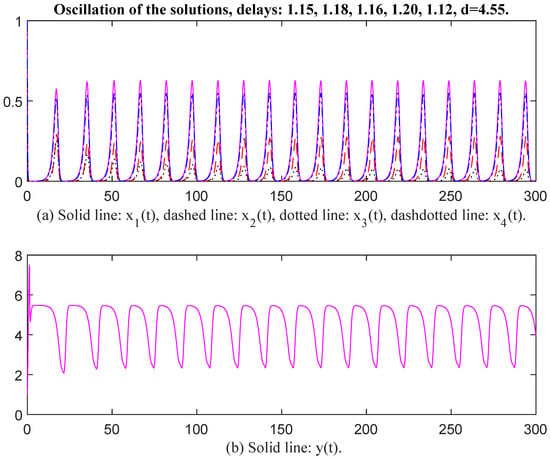
Figure 12. Oscillation of the solutions, delays: 1.15, 1.18, 1.16, 1.20, 1.12, d = 4.55.

5. Conclusions

In this paper, we have discussed the oscillatory behavior of the solutions for a cluster model with one core enterprise and four satellite enterprises. Based on the method of mathematical analysis, we provided two theorems to guarantee the oscillation of the solutions. Some simulations are provided to indicate the effectiveness of the criteria. It is found that all solutions are bounded under some selected parameter values. However, the upper bound of the core enterprise is greater than that of the satellite enterprises. It not only depends on its own production capacity but also depends on the production capacities of four satellite enterprises. It is also found that the production period plays a key role in the evolution of an enterprise cluster. Periodic oscillation of the solutions means that the enterprise cluster system displays a periodic fluctuation. As an enterprise manager, one must understand that output fluctuation may affect the stable development of enterprises and production efficiency. Controlling the production period in a suitable region is very important. Obviously, studying the dynamic behavior of a cluster model of any m core enterprises and any n satellite enterprises is very significant. This is our future work.

References

- Liao, M.; Xu, C.; Tang, X. Stability and Hopf bifurcation for a competition and cooperation model of two enterprises with delay. Commun. Nonlinear Sci. Numer. Simul. 2014, 19, 3845–3856. [Google Scholar] [CrossRef]
- Zhang, X.; Zhang, Z.H.; Wade, M.J. Dynamical analysis of a competition and cooperation system with multiple delays. Bound. Value Prob. 2018, 2018, 111. [Google Scholar] [CrossRef]
- Muhammadhaji, A.; Nureji, M. Dynamical behavior of competition and cooperation dynamical model of two enterprises. J. Quant. Econ. 2019, 36, 94–98. [Google Scholar]
- Xu, C.J.; Shao, Y.F. Existence and global attractivity of periodic solution for enterprise clusters based on ecology theory with impulse. J. Appl. Math. Comput. 2012, 39, 367–384. [Google Scholar] [CrossRef]
- Muhammadhaji, A.; Maimaiti, Y. New criteria for analyzing the permanence, periodic solution, and global attractiveness of the competition and cooperation model of two enterprises with feedback controls and delays. Mathematics 2023, 11, 4442. [Google Scholar] [CrossRef]
- Xu, C.J.; Li, P.L.; Xiao, Q.M.; Yuan, S. New results on competition and cooperation model of two enterprises with multiple delays and feedback controls. Bound. Value Prob. 2019, 2019, 36. [Google Scholar] [CrossRef]
- Lu, L.; Lian, Y.; Li, C. Dynamics for a discrete competition and cooperation model of two enterprises with multiple delays and feedback controls. Open Math. 2017, 15, 218–232. [Google Scholar] [CrossRef]
- Guerrini, L. Small delays in a competition and cooperation model of enterprises. Appl. Math. Sci. 2016, 10, 2571–2574. [Google Scholar] [CrossRef]
- Jiang, Y.L.; Ji, L.H.; Liu, Q.; Yang, S.S.; Liao, X.F. Couple-group consensus for discrete-time heterogeneous multiagent systems with cooperative–competitive interactions and time delays. Neurocomputing 2018, 319, 92–101. [Google Scholar] [CrossRef]
- Xu, C.; Li, P. Almost periodic solutions for a competition and cooperation model of two enterprises with time-varying delays and feedback controls. J. Appl. Math. Comput. 2017, 53, 397–411. [Google Scholar] [CrossRef]
- Li, Y.K.; Zhang, T. Global asymptotical stability of a unique almost periodic solution for enterprise clusters based on ecology theory with time-varying delays and feedback controls. Commun. Nonlinear Sci. Numer. Simul. 2012, 17, 904–912. [Google Scholar] [CrossRef]
- Peng, C.; Li, X.L.; Du, B. Positive periodic solution for enterprise cluster model with feedback controls and time-varying delays on time scales. AIMS Math. 2024, 9, 6321–6335. [Google Scholar] [CrossRef]
- Ren, J.; Sun, H.; Xu, G.J.; Hou, D.S. Convergence of output dynamics in duopoly co-opetition model with incomplete information. Math. Comput. Simul. 2023, 207, 209–225. [Google Scholar] [CrossRef]
- Ren, J.; Sun, H.; Xu, G.J.; Hou, D.S. Prediction on the competitive outcome of an enterprise under the adjustment mechanism. Appl. Math. Comput. 2020, 372, 124969. [Google Scholar] [CrossRef]
- Alfifi, H.Y. Effects of diffusion and delays on the dynamic behavior of a competition and cooperation model. Mathematics 2025, 13, 1026. [Google Scholar] [CrossRef]
- Alfifi, H.Y.; Almuaddi, S.M. Stability analysis and hopf bifurcation for the Brusselator reaction—Diffusion system with gene expression time delay. Mathematics 2024, 12, 1170. [Google Scholar] [CrossRef]
- Muhammadhaji, A.; Teng, Z.; Rahim, M. Dynamical behavior for a class of delayed competitive-mutualism systems. Differ. Equ. Dyn. Syst. 2015, 23, 281–301. [Google Scholar] [CrossRef]
- Guo, J.S.; Guo, K.R.; Shimojo, M. Forced waves for diffusive competition systems in shifting environments. Nonlinear Anal. RWA 2023, 73, 103880. [Google Scholar] [CrossRef]
- Chen, Y.S.; Guo, J.S. Traveling wave solutions for a three-species predator–prey model with two aborigine preys. Jpn. J. Ind. Appl. Math. 2021, 38, 455–471. [Google Scholar] [CrossRef]
- Li, X.S.; Pan, S.X. Traveling wave solutions of a delayed cooperative system. Mathematics 2019, 7, 269. [Google Scholar] [CrossRef]
- Wei, Z.Z.; Zhang, X. Dynamics of a diffusive delayed competition and cooperation system. Open Math. 2020, 18, 1230–1249. [Google Scholar] [CrossRef]
- Konig, T. Between collaboration and competition: Co-located clusters of different industries in one region-the context of Tuttlingen’s medical engineering and metal processing industries. Reg. Sci. Poli. Prac. 2023, 15, 236–288. [Google Scholar] [CrossRef]
- Zeng, S.; Bao, J. Analysis of the effects of digital transformation of enterprise clusters on innovation performance in the context of “Internet+”. Syst. Soft Comput. 2025, 7, 200270. [Google Scholar] [CrossRef]
- Hu, W.J.; Dong, T.; Zhao, H. Dynamic analysis of a competition-cooperation enterprise cluster with core-satellite structure and time delay. Complexity 2021, 2021, 6644292. [Google Scholar] [CrossRef]
- Chafee, N. A bifurcation problem for a functional differential equation of finite retarded type. J. Math. Anal. Appl. 1971, 35, 312–348. [Google Scholar] [CrossRef]
- Feng, C.; Plamondon, R. An oscillatory criterion for a time delayed neural network model. Neural Netw. 2012, 29, 70–79. [Google Scholar] [CrossRef]
Disclaimer/Publisher’s Note: The statements, opinions and data contained in all publications are solely those of the individual author(s) and contributor(s) and not of MDPI and/or the editor(s). MDPI and/or the editor(s) disclaim responsibility for any injury to people or property resulting from any ideas, methods, instructions or products referred to in the content. |
© 2026 by the author. Licensee MDPI, Basel, Switzerland. This article is an open access article distributed under the terms and conditions of the Creative Commons Attribution (CC BY) license.