Mind the Gap: A Solution to the Robustness Problem of Turing Patterns Through Patterning Mode Isolation

Abstract

Turing patterns, characterised by spatial self-organisation in reaction–diffusion systems, exhibit sensitivity to initial conditions. This sensitivity, known as the robustness problem, results in different final patterns emerging even from small initial perturbations. In this paper, we introduce a mechanism of pattern mode isolation, where we investigate parameter regimes that promote the isolation of bifurcation branches, thereby delineating the conditions under which distinct pattern modes emerge and evolve independently. Pattern mode isolation can provide a means of enhancing the predictability of Turing pattern mode transitions and enhance the robustness and reproducibility of the patterning outputs.

1. Introduction

Turing patterns, first proposed by Alan Turing in 1952 [1,2,3], offer a compelling theoretical framework for understanding the emergence of spatial patterns in biological systems. From the fairly simple and biologically feasible set up of interacting populations (known as morphogens) Turing patterns can occur in spatially extended systems due to the intricate interactions of morphogen diffusion and interspecies dynamics. Depending on the spatial dimension in which the interactions are occurring, patterns in the morphogen populations, such as spots, stripes, or labyrinthine structures can appear [4]. Critically, neither the reaction kinetics nor the diffusion of the morphogens leads to patterning separately. It is only through their integration that the patterning is observed, meaning that Turing patterns are only possible because the dynamics of a reaction–diffusion system is more than the sum of its parts [5].

Turing patterns have garnered significant interest across diverse scientific disciplines due to their potential applications in various fields, such as developmental biology, materials science, and chemical engineering [4,6,7,8]. In developmental biology, Turing mechanisms have been implicated in the formation of complex tissue structures and morphogen gradients during embryonic development [9,10]. Moreover, Turing patterns have inspired novel approaches in materials science, particularly in the design and fabrication of biomimetic patterns for functional surfaces [11,12,13].

Beyond applications, the mathematical framework of Turing patterns has undergone extensive exploration, with extensions to non-standard reaction–diffusion models incorporating additional complexities, such as advection, cross-diffusion, or time delays [14,15,16]. These mathematical extensions provide deeper insights into pattern formation mechanisms and broaden the scope of Turing pattern theory in theoretical biology and applied mathematics.

Critically, Turing patterns are notoriously sensitive to initial conditions, a characteristic that poses challenges for their practical application in various biological and chemical contexts (see Figure 1) [17]. Under general kinetics and parameter values, many final possible spatial patterning solutions can exist. An example of this solution multiplicity is illustrated in Figure 1a, where the simulations were run under exactly the same parameters, but the initial conditions were uniformly randomly varied. We observe that five possible solutions (including symmetries) exist and we name them $n=5$ to $n=9$, respectively. This naming convention is in reference to the underlying wave mode that destabilises in their Fourier representation, but this will be clarified later in Section 3.

Since it is often assumed that the initial conditions of a Turing patterning simulation is a noisy input (usually random fluctuations around a uniform homogeneous steady state of the reaction kinetics) we cannot guarantee which of the five solutions we will evolve to. Moreover, as shown in Figure 1b, the distribution of the final patterns is not uniformly spread across the potential solutions since within ${10}^4$ simulations with random initial conditions, over half of all solutions look like an $n=7$ pattern (including symmetries), whilst only two simulations evolved to an $n=5$ pattern. This sensitivity to initial conditions is known as the robustness problem.

Although robustness is important when consistent pattern reproduction is essential [18], there are certain biological situations where sensitivity to initial conditions is not a drawback, but rather a beneficial feature [19]. For instance, in the context of animal coat patterns and fingerprints, individuality and diversity within species is a required feature for any patterning mechanism [20]. However, we are looking to consider cases, such as tooth formation, digit formation and feather placement [21,22], which are generally highly consistent in their output, even in the face of intraspecies variation.

Previous studies [23,24] showed that domain growth could potentially mitigate the sensitivity of Turing patterns to initial noise. Specifically, it was proposed that under optimal growth rates, pattern modes would naturally double with increasing domain size. It should be noted that under these optimal growth rates domain size can be effectively taken as a stationary bifurcation parameter which can be varied. However, non-optimal growth rates can disrupt the mode doubling process, emphasising the intricate dependency of pattern formation on spatial dynamics (see Figure 3) [25,26,27]. A more complete view of time-dependent growth rate theory can be seen in [28]. Here, we focus on the time-independent theory, which allows us to derive clear patterning domain boundaries that work in these intervals of optimal growth rates.

Additionally, noise, while typically considered detrimental to pattern formation, has been demonstrated to act as a catalyst for transitions between stable solution branches, effectively driving the system towards higher-order pattern modes [29]. However, the presence of multiple solution branches introduces ambiguity, as noise-induced transitions may not reliably progress the pattern to a specific next patterning mode [30,31].

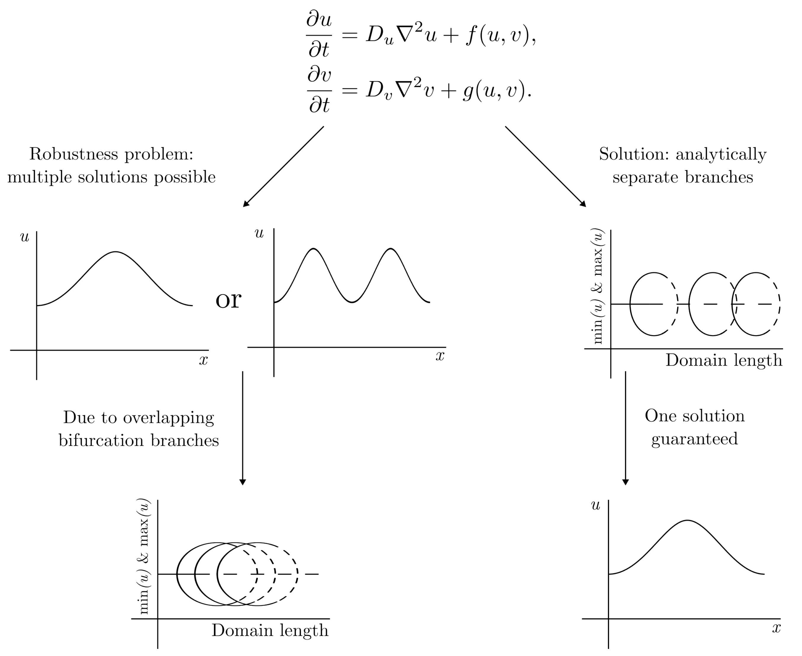
In this work, we aim to provide another potential solution to the robustness problem (see Figure 2), which solves a number of the problems of the presently suggested methods, although it does introduce its own shortcomings due to weaknesses of parameter fine-tuning. Specifically, we use linear analysis, simulation and bifurcation tracking to investigate under what conditions we can generate isolated bifurcation branches, thereby delineating the conditions under which distinct pattern modes emerge and evolve independently.

Figure 2. Graphically illustrating the problem and proposed solution. Pattern formation through reaction–diffusion equations generically leads to a robustness problem, where multiple patterns in $(u,v)$ are possible over the spatial variable, x. We show how to isolate the bifurcation branches at each domain size (stable solution branches are illustrated as solid line, whereas unstable solution branches are illustrated as dashed lines) leading to one guaranteed solution.

Figure 2. Graphically illustrating the problem and proposed solution. Pattern formation through reaction–diffusion equations generically leads to a robustness problem, where multiple patterns in $(u,v)$ are possible over the spatial variable, x. We show how to isolate the bifurcation branches at each domain size (stable solution branches are illustrated as solid line, whereas unstable solution branches are illustrated as dashed lines) leading to one guaranteed solution.

Figure 3. Simulations of Equations (7) and (8) with kinetics of Equations (5) and (6) demonstrating the influence of uniform exponential domain growth, when mapped back to the initial domain width, $l=4$. The left plots illustrate the pattern transitions in u as time increases. The right plot shows the bifurcation structure of the PDEs over L. The blue lines represent the maxima and minima of the solutions available at each value of L. The thick lines represent the stable solutions, whilst the thin lines represent the unstable solutions. The number against each line provides the wave mode name of each solution branch (explained in Section 3). The black line represents the maximum and minimum present in the left simulation under the mapping $L=lexp\left(rt\right)$. Parameters are $l=4$, $D_u=1$, $D_v=100$, $\beta =1.1$ and $\gamma =1.45$. The growth rate, r, is noted below each subfigure.

Figure 3. Simulations of Equations (7) and (8) with kinetics of Equations (5) and (6) demonstrating the influence of uniform exponential domain growth, when mapped back to the initial domain width, $l=4$. The left plots illustrate the pattern transitions in u as time increases. The right plot shows the bifurcation structure of the PDEs over L. The blue lines represent the maxima and minima of the solutions available at each value of L. The thick lines represent the stable solutions, whilst the thin lines represent the unstable solutions. The number against each line provides the wave mode name of each solution branch (explained in Section 3). The black line represents the maximum and minimum present in the left simulation under the mapping $L=lexp\left(rt\right)$. Parameters are $l=4$, $D_u=1$, $D_v=100$, $\beta =1.1$ and $\gamma =1.45$. The growth rate, r, is noted below each subfigure.

2. Framework

We consider two morphogen populations, $(u,v)$, that are able to diffuse with rates $(D_u,D_v)$ and interact under smooth kinetics $f(u,v)$ and $g(u,v)$, respectively, in an N-dimensional finite, bounded space $\Omega \in {\mathbb{R}}^N$ with boundary $\partial \Omega$. Assuming that the system is insulated and, thus, satisfies zero-Neumann boundary conditions, the evolution of the morphogens at a point $\mathit{x}\in \Omega$ and time $t>0$ is defined by the partial differential equations (PDEs).

$$\begin{array}{cc}\hfill {\displaystyle \frac{\partial u}{\partial t}}& =D_u{\nabla }^{2}u+f(u,v),\hfill \end{array}$$

(1)

$$\begin{array}{cc}\hfill {\displaystyle \frac{\partial v}{\partial t}}& =D_v{\nabla }^{2}v+g(u,v),\hfill \end{array}$$

(2)

$$\begin{array}{cc}\hfill {\displaystyle \frac{\partial u}{\partial n}}(\mathit{x},t)& ={\displaystyle \frac{\partial v}{\partial n}}(\mathit{x},t)=0,\mathrm{for}\mathit{x}\in \partial \Omega ,\hfill \end{array}$$

(3)

where ${\nabla }^2$ is the Laplacian.

To close the system, we must define initial conditions. To define the initial conditions we must first appeal to our assumption that the system is able to undergo a Turing instability. Namely, there exists a spatially uniform steady state $(u_s,v_s)$ of Equations (1)–(3) that is stable in the absence of diffusion, but can be driven unstable in the presence of diffusion. From this assumption we state that the initial conditions are

$$(u(\mathit{x},0),v(\mathit{x},0))=\left(\right|u_s+r_u\left(\mathit{x}\right)|,|v_s+r_v\left(\mathit{x}\right)\left|\right),$$

(4)

where $r_u$ and $r_v$ are sampled at every point, $\mathit{x}\in \Omega$, from a Normal distribution with zero mean and variance ${\sigma }^2=0.1$.

Although we will derive our results, in general, we will demonstrate our results using a modified form of the nondimensionalised Schnakenberg kinetics [32],

$$\begin{array}{cc}\hfill f(u,v)& =\gamma -\beta -u+u^{2}v,\hfill \end{array}$$

(5)

$$\begin{array}{cc}\hfill g(u,v)& =\beta -u^{2}v,\hfill \end{array}$$

(6)

where $\gamma >\beta >0$. The stereotypical form of the Schnakenberg kinetics replaces $\gamma -\beta$ with $\alpha =\gamma -\beta >0$. However, the change to $\gamma$, rather than $\alpha$ does not alter the pertinent parameter region, but it does allow us to simplify the resulting mathematical expressions. For example, the steady states of Equations (5) and (6) are $(\gamma ,\beta /{\gamma }^2)$, rather than $(\alpha +\beta ,\beta /{(\alpha +\beta )}^2)$.

Notably, going forward we will simplify our analysis by restricting the work to a one-dimensional domain of length L, $\Omega =[0,L]$. Although the analysis can be performed in higher dimensions, we also generate more patterning possibilities, which can be stable at the same time [33,34,35]. We will discuss this more at length when the spatial perturbation is introduced in Section 3 and we are able to discuss wave modes and wave vectors.

Domain Growth

As mentioned in Section 1, one possible solution to the robustness problem was to cast the pattern formation system onto a growing domain. Specifically, symmetry arguments could be shown that exponentially fast domain growth led to a pattern doubling mechanism [36,37].

Including domain growth in the reaction–diffusion PDE framework requires us to return to the fundamentals of the derivation, where we consider the flux of material across the boundary of an evolving arbitrary test volume and requires Reynold’s transport theorem [28,38]. Furthermore, simulating reaction–diffusion equations on growing domains is difficult, as mesh movement and coarsening has to be accounted for [25]. Thus, it is much easier from an analytical and simulation front to map a growing domain, $[0,L(t\left)\right]$, to a stationary domain, $[0,l]$ through a spatial scaling that leads to a rescaling of the PDEs, making them non-autonomous. This process is further simplified if we assume uniform domain growth [39], as each point, $x\left(t\right)\in [0,L(t\left)\right]$, in the evolving space can be mapped directly back to the stationary space, $X\in [0,l]$, through $x\left(t\right)=L\left(t\right)X/l$.

Although important, we suppress further derivation and leave the details to the referenced publications because the final form of the PDE system is a simple extension of Equations (1) and (2), which the full derivation tends to obfuscate. Namely, the analogous system of Equations (1) and (2) on a domain growing uniformly exponentially, with rate r, $L\left(t\right)=lexp\left(rt\right)$, once mapped to the stationary domain $[0,l]$ is [24]

$$\begin{array}{cc}\hfill {\displaystyle \frac{\partial u}{\partial t}}& ={\displaystyle \frac{D_u}{exp\left(2rt\right)}}{\nabla }^{2}u+f(u,v)-ru,\hfill \end{array}$$

(7)

$$\begin{array}{cc}\hfill {\displaystyle \frac{\partial v}{\partial t}}& ={\displaystyle \frac{D_v}{exp\left(2rt\right)}}{\nabla }^{2}v+g(u,v)-rv.\hfill \end{array}$$

(8)

Boundary and initial conditions are the same as in the initial system.

The left image of Figure 3a illustrates the pattern doubling phenomenon that occurs when Turing systems are simulated on exponentially growing domains. Initially, we start the domain too small to pattern, but over time a peak on the boundary appears (an $n=1$ wave mode pattern), this transitions into a single peak in the centre of the domain (an $n=2$ wave mode pattern) and the pattern doubling cascade continues, producing a two peak and a four peak solution (an $n=4$ and $n=8$ wave mode pattern, respectively) through each peak splitting into two daughter peaks during the rapid transition phases.

Using pde2path 2.0 [40,41], we are able to numerically extract the bifurcation structure of Equations (1) and (2) using the domain size as a bifurcation parameter [42], see the right-hand plots of Figure 3. The blue lines present the maxima and minima of all steady state solutions of Equations (7) and (8) with kinetics Equations (5) and (6). The thick lines represent the stable solutions, whilst the thin lines represent the unstable solutions. Note, we are only showing the solution branches that bifurcate from the uniform steady state and only branches that contain stable solutions. Isolated branches of unstable solutions do exist, but are not relevant to our interests [43].

For a fixed domain length, the thick blue lines predict the possible Turing pattern solutions that can be generated. Thus, we can use the bifurcation diagrams in Figure 3 to support the results of Figure 1. For a domain length of $L=60$ the bifurcation diagram shows that wave modes n = 5–9 are all possible, as shown in Figure 1a. Moreover, we can see that we are at the very end of the stable region of the wave mode $n=5$ branch. Equally, we are very close to the start of the stability region of the $n=9$ branch. This means we are very close to the point at which these two solutions would not exist and, in some sense, they are ‘less stable’ than the other available solutions, which explains why the $n=5$ and 9 solutions are seen so infrequently amongst the ${10}^4$ simulations of Figure 1b.

The bifurcation structure also provides an alternative approach to understanding the pattern evolution of Turing systems on growing domains [43]. The right image of Figure 3a illustrates the comparison between the growing domain simulation and the bifurcation structure. The black trajectory over the top of the blue lines represents the maxima and minima of the simulation in the left image of Figure 3a.

Firstly, we observe that the maxima and minima of the solution match the predicted bifurcation structure. Secondly, whilst a trajectory is tracking a stable branch, it remains on that branch even in the face of other solutions being available. Finally, the solution only leaves a branch when the branch destabilises. The solution then quickly transitions to another stable branch, in particular, due to the doubling phenomenon, only the branches $n=1,2,4$, and 8 are followed.

Although Figure 3a presents the expected solution that does occur across a wide interval of growth rates the doubling phenomenon can break down if the growth rate is too slow, or too fast, see Figure 3b,c, respectively. For example, in Figure 3b where the growth rate is orders of magnitude slower than Figure 3a, we see that the first two transitions along wave modes $n=1$ and 2 still occur. However, because the growth is so slow the trajectory spends too long in the window between wave mode 2 destabilising and wave mode 4 stabilising and, so, the trajectory evolves to a wave mode 3 pattern, breaking the doubling pattern.

In comparison, when the growth is too fast in Figure 3c wave modes are skipped because the solution is unable to stabilise onto a particular branch before the branch disappears. For example, from the left plot of Figure 3c it appears that the solution is tending to a wave mode three solution; however, in the right plot of Figure 3c we see that the trajectory never manages to reach the $n=3$ branch before it disappears, when $L\left(t\right)\approx 40$, or $t\approx 115$.

In summary, one reason for the breakdown of the robust pattern doubling seen in Figure 3 is that the bifurcation branches overlap one another. Any perturbation to a solution trajectory can lead to the solution not successfully moving between the pattern doubling branches. The solutions will be particularly susceptible to perturbations altering their evolution during the reorganisation phase of moving between the one stable branch and another. In the following sections we derive conditions under which we can separate the forest of bifurcation branches ensuring that at most one mode is available at any time.

3. Turing Conditions

There are many sources for the derivation of the Turing conditions [4] under many extensions [44,45]. We include a brief derivation for completeness and it will allow us to focus on the key condition that enables wave mode isolation.

Having specified that Equations (1)–(3) have a spatially uniform steady state we need to ensure that (i) the state is stable when the diffusion rates are zero and (ii) an instability can occur when they are not. We will be approaching the analysis through linearisation [46]; however, we will also be including bifurcation diagrams that are generated through simulation. Although parts of the bifurcation diagram can be understood using weakly nonlinear analysis and singular perturbation theory [47] the full features of the system are not tractable and require simulation.

In case (i), we set $D_u=D_v=0$, so, we can simply remove spatial considerations from system (1)–(3) and treat the system as a pair of coupled ordinary differential equations. Substituting in a perturbation of the steady state,

$$\left(\begin{array}{c}\hfill u(\mathit{x},t)\\ \hfill v(\mathit{x},t)\end{array}\right)=\left(\begin{array}{c}\hfill u_s\\ \hfill v_s\end{array}\right)+\left(\begin{array}{c}\hfill {ϵ}_u\\ \hfill {ϵ}_v\end{array}\right)exp\left(\lambda t\right),$$

and assuming that $0<{ϵ}_u<{ϵ}_v\ll 1$, we can expand the system in terms of $({ϵ}_u,{ϵ}_v)$ near the steady state. To first order in $({ϵ}_u,{ϵ}_v)$ we derive that $\lambda$, whose sign determines the stability characteristics of the steady state satisfies the following eigenvalue problem

$$\mathit{J}\left(\begin{array}{c}\hfill {ϵ}_u\\ \hfill {ϵ}_v\end{array}\right)=\lambda \left(\begin{array}{c}\hfill {ϵ}_u\\ \hfill {ϵ}_v\end{array}\right),$$

(9)

where $\mathit{J}$ is the matrix of first order derivatives, known as the Jacobian,

$$\mathit{J}={\left.\left(\begin{array}{c}\hfill f_u,f_v\\ \hfill g_u,g_v\end{array}\right)\right|}_{(u_s,v_s)},$$

which we assume is not the zero matrix. Explicitly, we note that all the partial derivatives in the Jacobian and the following results are evaluated at the steady state, $(u_s,v_s)$. Equation (9) implies that the Jacobian minus the identity matrix must be singular; thus, its determinant must be zero, resulting in a quadratic equation for $\lambda$, which can be solved to give

$${\lambda }_{\pm }={\displaystyle \frac{f_u+g_v\pm \sqrt{{(f_u+g_v)}^2-4(f_u{g}_v-g_u{f}_v)}}{2}}.$$

(10)

To ensure stability we require that the real parts of ${\lambda }_{\pm }$ are negative leading to the first two patterning conditions,

$$\begin{array}{c}{f}_u+g_v<0,\end{array}$$

(11)

$$\begin{array}{c}{f}_u{g}_v-f_v{g}_u>0.\end{array}$$

(12)

Critically, since inequalities (11) and (12) are derived in the absence of spatial considerations they need to be satisfied regardless of our wave mode isolation intentions.

Having derived conditions to satisfy case (i), we return to Equations (1)–(3) and consider case (ii), which requires conditions under which an instability can occur when $D_u\ne 0\ne D_v$. In this case, we use a spatial perturbation of the form

$$\left(\begin{array}{c}\hfill u(\mathit{x},t)\\ \hfill v(\mathit{x},t)\end{array}\right)=\left(\begin{array}{c}\hfill u_s\\ \hfill v_s\end{array}\right)+\left(\begin{array}{c}\hfill {ϵ}_u\\ \hfill {ϵ}_v\end{array}\right)exp\left(\lambda t\right)cos\left(kx\right),$$

(13)

where $cos\left(kx\right)$, $k=n\pi /L,n\in \mathbb{Z}$ is used because it satisfies the Laplacian with zero-Neumann boundary conditions. At this point we are able to define n as the wave mode of a solution, an intuitive way of seeing this is how many ‘half peaks’ make up a solution. For a concrete example, consider the solutions in Figure 1a. The left-hand solution has 2.5 peaks, which is why it is called a wave mode 5 pattern, whilst the right-hand solution has 4.5 peaks, meaning it is a wave mode 9 solution.

At this point, we can expand on the difficulties mentioned above for higher dimensions. In one dimension, only peak and trough patterns appear and k is a scalar. In two dimensions, spots, stripes, and labyrinthine patterns appear, meaning that we need to consider the wave modes in at least two directions. For example, on a two-dimensional rectangle of size $L_x\times L_y$ we would need to consider spatial perturbations of the form $cos(\mathit{k}·\mathit{x})$, where $\mathit{k}=(k_x,k_y)=(n\pi /L_x,m\pi /L_y)$ measures the frequencies in the two Cartesian directions. However, when considering the linearisation Equations (1) and (3) the analysis only depends on the magnitude of $\mathit{k}$, $k^2={\left|\mathit{k}\right|}^2=k_x^2+k_y^2={(n\pi /L_x)}^2+{(m\pi /L_y)}^2$. Thus, there are solutions for the same value of ${\left|\mathit{k}\right|}^2$, which have different values of m and n. The interpretation of this is that spots can have multiple arrangements (e.g., square, hexagonal, or rhombic) each with their own stability characteristics. Hence, although the analysis could be extended to higher dimensions, we would need to use weakly nonlinear analysis to derive conditions through which we can ensure that only one pattern arrangement would be stable at a time [35,48].

Noting this limitation, we continue in one dimension and substitute perturbation (13) into Equations (1) and (3). Expanding to first order in $({ϵ}_u,{ϵ}_v)$ produces the following consistency equation,

$$\left(\mathit{J}-\left(\begin{array}{cc}{k}^2{D}_u+\lambda & 0\\ 0& k^2{D}_v+\lambda \end{array}\right)\right)\left(\begin{array}{c}\hfill {ϵ}_u\\ \hfill {ϵ}_v\end{array}\right)=0.$$

(14)

Since ${ϵ}_u$ and ${ϵ}_v$ are not both zero, then Equation (14) can only be solved if the prefactor matrix is singular. Extracting the matrix’s determinant and setting it to zero leads to the dispersion relation,

$${\lambda }^2+\lambda (k^2(D_u+D_v)-f_u-g_v)+(k^2{D}_u-f_u)(k^2{D}_v-g_v)-g_u{f}_v=0.$$

(15)

We could solve Equation (15) for $\lambda$; however, the result becomes cumbersome. Instead, it is easier to apply the Routh–Hurwitz condition [49], which says that Equation (15) has negative roots if and only if the coefficients of each $\lambda$ term and the constant coefficient are positive. Since inequality (11) is required, then the coefficients of ${\lambda }^2$ and $\lambda$ are guaranteed to be positive. Hence, the only means of producing a root of Equation (15) with a positive real component (ensuring instability) is to ensure that the constant term is negative,

$$h\left(k^2\right)=(k^2{D}_u-f_u)(k^2{D}_v-g_v)-g_u{f}_v=k^4{D}_u{D}_v-k^2(D_u{g}_v+D_v{f}_u)+f_u{g}_v-g_u{f}_v<0.$$

(16)

Ensuring that Equation (16) is satisfiable produces the last two patterning criteria

$$D_u{g}_v+D_v{f}_u>2\sqrt{D_u{D}_v(f_u{g}_v-g_u{f}_v)}>0.$$

(17)

Assuming that inequality (17) can be satisfied means that h is quadratic in $k^2$ with two positive roots,

$$k_{\pm }^2={\displaystyle \frac{D_u{g}_v+D_v{f}_u\pm \sqrt{{(D_u{g}_v+D_v{f}_u)}^2-4D_u{D}_v(f_u{g}_v-g_u{f}_v)}}{2D_u{D}_v}}.$$

(18)

However, it is not enough for the roots to exist. Due to the discrete form of the admissible wave modes, $k=n\pi /L$, we must also guarantee that there are positive integers, n, such that

$$k_{-}^2\le {(n\pi /L)}^2\le k_{+}^2.$$

(19)

In summary, the linear analysis shows that diffusion has the potential to destabilise a uniform steady state only within a specific window of admissible spatial frequencies. This window is determined entirely by the coefficients of the kinetic Jacobian and the diffusion rates. The inequalities (11) and (19) collectively specify when such a patterning window exists and which discrete modes on a finite domain fall inside the interval. Hence, once these conditions are satisfied, the task of controlling pattern formation reduces to understanding how wide this instability window is and how many discrete wave modes it can contain.

If we have freedom to choose the size of the domain, then satisfying inequality (19) is not difficult as it can be readily satisfied by choosing a large enough L. However, choosing a large L will usually mean that there are multiple wave modes, n, that will satisfy inequality (19) (see Figure 4). Indeed, for any set of parameter values there will be a domain large enough such that multiple wave modes are unstable. However, for a fixed L, it may be possible to choose parameter values such that all wave modes less than an arbitrary integer are isolated as in the right image of Figure 4.

The key idea is that the number of possible patterns is dictated not by the overall size of the domain but by how many discrete wave modes fall within the unstable interval. By shrinking this interval, fewer (and eventually only one) integer wave modes remain admissible. This converts a system with many competing patterning outcomes into one where the dynamics must evolve onto a single mode. In summary, mode isolation is mathematically equivalent to compressing the instability window so that it contains only one allowable spatial frequency.

4. Mode Isolation

From Figure 4, we observe that the key to isolating modes is to control the interval size, $k_{+}^2-k_{-}^2$, over which inequality (16) is satisfied. Thus, for this interval to be small we require that inequality (17) is not just satisfied, but the left and middle terms are approximately equal.

Considering a general integer mode $1\le n$ and its consecutive neighbours, the largest the root interval size can be and produce an isolated mode is

$${\displaystyle \frac{n\pi }{L_c}}=k_{-}<{\displaystyle \frac{(n+1)\pi }{L_c}}<k_{+}={\displaystyle \frac{(n+2)\pi }{L_c}},$$

(20)

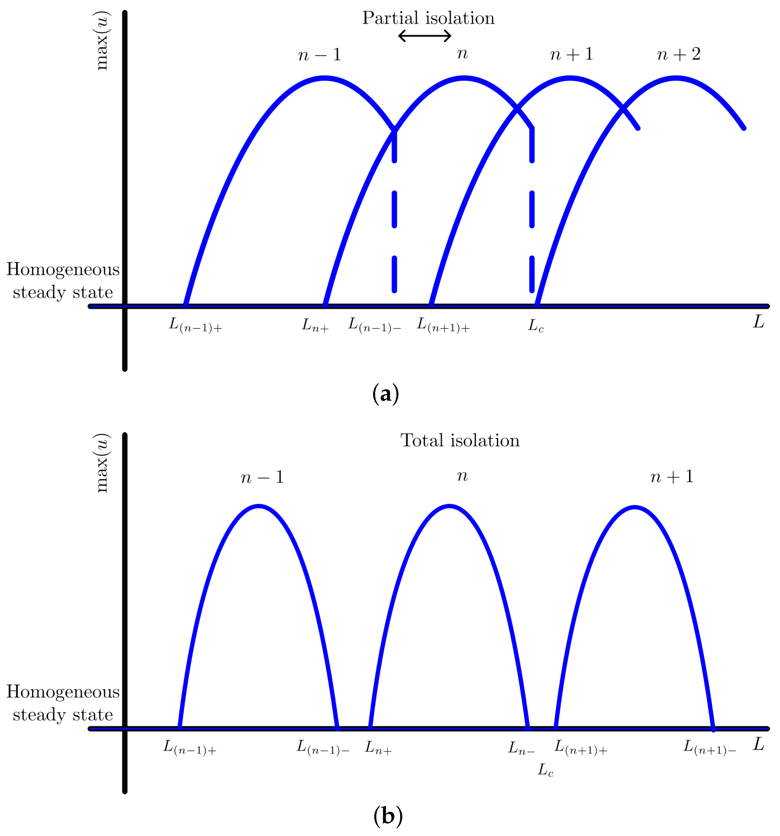
which ensures that at least at point $L=L_c$ the $n+1$ wave mode is isolated. However, for any larger, or smaller, L the $n+2$, or n, wave mode would also become stable, respectively (see Figure 5a).

Since the interval between wave modes increases as n decreases, this means that there will be a region of partial isolation for the $n^{th}$ wave mode. Explicitly, considering Figure 5 and defining the points $L_{i+}$ and $L_{i-}$ to be where the $i^{th}$ wave modes destabilise and stabilise, respectively, then if $L_c$ satisfies inequality (20) then $L_{(n-1)-}=L_c(n-1)/n$ and $L_{(n+1)+}=L_c(n+1)/(n+2)$. Since $(n-1)/n<(n+1)/(n+2)$ for all n then $L_{(n-1)-}<L_{(n+1)+}$ meaning that there will be some non-trivial interval where n is only stable wave mode (see Figure 5a). In this case, total isolation could occur when $L_{(n-1)-}<L_{n+}$, which occurs when $n/(n+2)>(n-1)/n$, or when $2>n$, meaning that the $n=1$ wave mode is the only wave mode that could be totally isolated.

Although partial isolation is useful as it leads to regions where only one wave mode is stable, there would still be regions of mixed modes, meaning the trajectory by which the modes appear may not be robust. We aim to generate wave mode chains as seen in Figure 5b, where each mode is totally isolated from the rest, ensuring that not only is each final wave mode guaranteed, but the transition to the wave mode is also ensured.

To achieve total mode isolation, we do not consider the widest possible interval. Indeed, for larger modes, n, to be isolated, we need to make the interval $[k_{-},k_{+}]$ smaller. Explicitly, we require that there exists some $L_c$ such that

$${\displaystyle \frac{n\pi }{L_c}}\le k_{-}<k_{+}\le {\displaystyle \frac{(n+1)\pi }{L_c}}.$$

(21)

Using an argument similar to the above, $L_c$ satisfies

$$\begin{array}{c}{L}_{n-}\le L_c\le L_{(n+1)+},\\ L_{(n-1)-}\le L_c{\displaystyle \frac{n-1}{n}}<L_c{\displaystyle \frac{n}{n+1}}\le L_{n+}.\end{array}$$

Since $L_{(n-1)-}<L_{n+}$ and $L_{n-}\le L_{(n+1)+}$ then the wave mode n stability interval is isolated as suggested by Figure 5b. Further, for any $1\le m<n$

$$L_{m-}\le L_c{\displaystyle \frac{m}{n}}<L_c{\displaystyle \frac{m+1}{n+1}}\le L_{(m+1)+}$$

(22)

meaning that the $m^{th}$ mode stability interval will also be isolated.

5. Simulation

As demonstrated in Section 4, mode isolation occurs if we can satisfy inequality (21) alongside all other Turing conditions (11)–(19). In this section, we use the modified Schnakenberg Equations (5) and (6) to demonstrate that we are able to satisfy inequality (21) for arbitrary wave modes, although higher wave mode isolation requires finer tuning of the parameters.

Firstly, the Turing conditions in the scenario are

$$\begin{array}{c}2\beta -\gamma (1+{\gamma }^2)<0,\end{array}$$

(23)

$$\begin{array}{c}{\gamma }^2>0,\end{array}$$

(24)

$$\begin{array}{c}-{\gamma }^3+(2\beta -\gamma )D>2\sqrt{D}{\gamma }^2,\end{array}$$

(25)

$$\begin{array}{c}{k}_{-}^2\le {(n\pi /L)}^2\le k_{+}^2,\mathrm{such}\mathrm{that}{k}_{\pm }^2={\displaystyle \frac{-{\gamma }^2+(2\beta -\gamma )D/\gamma \pm \sqrt{{(-{\gamma }^2+(2\beta -\gamma )D/\gamma )}^2-4D{\gamma }^2}}{2D}},\end{array}$$

(26)

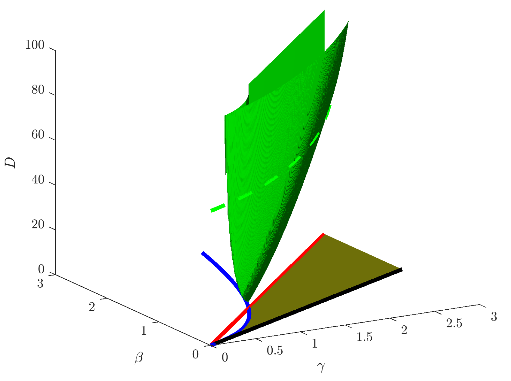
where $D=D_v/D_u$. Figure 6 illustrates inequalities (23)–(25) providing an illustration of the Turing patterning parameter region. We note that Turing parameter region is unbounded, such that for $(\gamma ,\beta )$ satisfying inequalities (23)–(25) (occurring in the green plane of Figure 6) there will be a $D_{\min }$ such that inequality (25) will be satisfied for all $D>D_{\min }$. However, although patterns are theoretically possible, numerical simulations may be difficult in cases of extremely large D. Another point to note about Figure 6 is that the dashed green line on the boundary of the green shell represents $g_v+D{f}_u=2\sqrt{D(f_u{g}_v-g_u{f}_v)}$, thus, parameters must be chosen close to the boundary linked to this dashed line for isolated modes to appear.

Using inequality (21), we can solve for the following two variables

$$\begin{array}{c}{\beta }_n(\gamma ,D,n)={\displaystyle \frac{{\gamma }^3}{2D}}+{\displaystyle \frac{\left(2n^2+2n+1\right){\gamma }^2}{2n\left(n+1\right)\sqrt{D}}}+{\displaystyle \frac{\gamma }{2}},\end{array}$$

(27)

$$\begin{array}{c}L(\gamma ,D,n)={\displaystyle \frac{\pi D^{1/4}}{\sqrt{\gamma }}}\sqrt{n(n+1)},\end{array}$$

(28)

which generate the wave mode boundary lines. Since we are considering L to be a parameter, the space between the ${\beta }_n$ curves tells us that mode isolation is possible for some L. Specifically, ${\beta }_n$ and ${\beta }_{n+1}$ provide us with boundary curves between which the wave mode n is destabilised and isolated. Moreover, between ${\beta }_n$ and ${\beta }_{n+1}$ all wave modes less than n are also isolated, for some L. In practical terms, the functions ${\beta }_n(\gamma ,D,n)$ and $L(\gamma ,D,n)$ provide a way of locating, in advance, where mode isolation will occur. Rather than searching numerically for isolated branches, these expressions tell us which combinations of $(\gamma ,\beta )$ will cause the instability window to narrow around a single admissible wave mode (see Figure 7).

The ${\beta }_n$ curves are illustrated in Figure 7a. As expected, the curves are within the Turing patterning parameter region and very close to one another, becoming closer as n increases. Critically, for some D large enough all the ${\beta }_n$ shown satisfy inequality (25), with the inequality becoming an equality as $n\to \infty$. This can be seen particularly in the right of Figure 7a where we observe that the green dashed line is below the thin wave mode isolation boundary lines.

Using Figure 7a we extract several $(\gamma ,\beta )$ values, one between each of the ${\beta }_n$ boundaries for $n=1,\dots ,6$. In each case $\gamma =10$ and the accompanying $\beta$ values are listed in Figure 7b–f, which demonstrate the proposed principles of both partial and total mode isolation. Namely, the bifurcation diagrams in Figure 7b–f illustrate that the $n^{th}$ and all lower wave modes have isolated L regions of instability when the $\beta$ value is chosen between ${\beta }_n$ and ${\beta }_{n+1}$. This concept of mode isolation is further illustrated in Figure 7g, where we observe a very slowly growing domain. The parameters of Figure 7g match those of Figure 7f, thus, the first five wave modes should be isolated, corresponding to the observation that each of the first five patterns in Figure 7g have discrete regions over which they appear and disappear, but the wave mode $n=6$ pattern that occurs around $t\approx 17\times {10}^5$ transitions directly into the mode $n=7$ pattern at $t\approx 18\times {10}^5$.

6. Conclusions

In this paper, we have demonstrated that we can use the Turing patterning conditions to isolate wave modes, ensuring that only at most one pattern is available during a system’s evolution regardless of the initial randomness and other potential sources of noise that may occur, e.g., mode transitions that occur during growth. Not only does this solve the problem of robustness on a stationary domain, but it also aids the robustness when growth is considered, since, even in the case when the domain growth is ‘very slow’ the solution trajectory is only able to evolve to at most one pattern (compare with Figure 3).

Regarding growth, mode isolation is also a solution to the problem of generating non-doubled patterned states. For example, if we are to robustly generate the three digits of a chicken wing [50], or the five digits of a human, then period doubling generates its own problem as these two wave modes fall outside the doubling cascade of $n=1\to 2\to 4\to 8$. There have been suggestions of using logistic, or non-uniform domain growth [37,39], but neither of these guarantee the final pattern in the face of noise and/or perturbations to growth speed. In short, whilst multiple stable solution branches overlap, there is always the possibility of the solution not evolving along a precise trajectory.

Recognising the possibility of mode isolation as a means of enhancing robustness we must now face its limitations. Firstly, mode isolation will not solve the robustness problems generated by a fast-growing system. If the growth rate is faster than the speed of pattern formation, then no mode will stabilise and modes may be missed similar to Figure 3c.

Parameter fine-tuning is an obvious weakness of this method. Considering the results in Figure 7, we observe that all of our $\beta$ choices were within the interval $[8.71,93]$ and the interval of isolation is of size $|{\beta }_n-{\beta }_{n+1}|\propto \gamma /n^3$, thus, even if we could increase $\gamma$, or use different kinetics entirely, isolating higher order wave modes will always require fine-tuning.

Mathematically, this fine-tuning acts by reducing the width of the unstable interval $[k_{-}^2,k_{+}^2]$, since the term ${(Du{g}_v+Dv{f}_u)}^2-4D_u{D}_v(f_u{g}_v-g_u{f}_v)$ in Equation (18) approaches zero as $(\beta ,\gamma ,D)$ are brought closer to the (17) boundary (see Figure 4). In this regime the roots $k_{-}^2$ and $k_{+}^2$ coalesce, leaving at most one admissible $n\pi /L$ within the instability window. Consequently, each unstable branch becomes isolated in the bifurcation diagram, ensuring that the trajectory can only evolve onto a single predictable pattern mode and thereby enhancing the robustness of the final patterning output.

To counter the criticism of fine-tuning, we appeal to the complexity of biology and note that a two species PDE system is a simple caricature of the true nature of the system. Moreover, biology is known for having many buffering systems and multiple redundancies that ensure complex systems are kept within well-regulated limits, e.g., homeostasis [51,52]. Thus, it is not impossible for such fine-tuning to be within the realms of biological possibility.

Another potential criticism is that mode isolationism leads to regions of no patterns existing between isolated modes. Again, this reduces to a question of biological intention. Is it better to construct a patterning system that generates a pattern, even if it is the wrong one? Or is it better to ensure that at most one pattern is available? Different applications will require different approaches. For example, cancerous tumours release biochemical factors to encourage the rapid construction of new blood vessels that will transport oxygen to themselves. These new vessels are grown quickly and are often inefficient and leaky, with surplus grown to requirement. Thus, it is clear that the tumour values obtaining any oxygen it can, rather than carefully crafting an efficient transport system, which is antithetical to the way our body would normally construct blood vessels [53,54].

Physically testing the mode isolation mechanism could be achieved in reacting thin-film systems, or precipitation reactions, where the diffusion ratio and feed rates can be tuned directly. In such settings, reducing diffusion rates acts in a manner analogous to increasing the domain size, meaning that with sufficiently fine control the resulting patterns should reproduce the behaviour illustrated in Figure 7g. Biologically, the situation is more challenging because, outside synthetic or highly controlled systems, we rarely have precise experimental control over the governing kinetic and transport parameters. However, the presence of strong robustness across many developmental processes (for example, most humans consistently form ten toes, ten fingers, and a predictable limb arrangement) suggests that regulatory mechanisms exist to constrain pattern variability. In such cases, the proposed mode isolation mechanism becomes a plausible candidate for contributing to this robustness.

Whilst our analysis has focused on one-dimensional domains, the underlying mechanism extends naturally to two-dimensional and radial geometries. However, in higher spatial dimensions, wave modes are now vectors, leading to the possibility of multiple patterns being possible, e.g., spot and/or stripes. Thus, although the Turing analysis generalises readily to higher-dimensional domains meaning that the patterning stability intervals can be separated by judicious choice of fine-tuning the multiplicity of patterning modes would require a fuller, geometry-specific treatment.

Overall, this work establishes a new theoretical basis for understanding and engineering robustness in reaction–diffusion systems. Approaching pattern construction through mode isolation provides a flexible framework with potential applications across disciplines. For example, the mechanism offers a principled route for designing synthetic biological circuits, as well as chemical or materials-based systems, in which precise wavelength selection is needed to generate reproducible microstructural patterns under controlled laboratory conditions.

Looking ahead, our findings suggest several avenues for future research. Investigating more sophisticated models that capture the nuances of biological growth and pattern formation can provide deeper insights. Additionally, exploring methods to mitigate the limitations of mode isolation, such as integrating it with other robustness-enhancing techniques, could further improve pattern trajectory reproduction. Continued research in this area holds promise for advancing our understanding of biological pattern formation and developing practical applications in developmental biology.

References

1. Turing, A.M. The chemical basis of morphogenesis. Philos. Trans. R. Soc. Lond. B 1952, 237, 37–72. [Google Scholar] [CrossRef]
2. Woolley, T.E.; Baker, R.E.; Maini, P.K. Chapter 35: Turing’s theory of morphogenesis. In The Turing Guide; Sprevak, M., Copeland, J., Bowen, J.W.R., Eds.; Oxford University Press: Oxford, UK, 2017. [Google Scholar]
3. Krause, A.L.; Gaffney, E.A.; Maini, P.K.; Klika, V. Modern perspectives on near-equilibrium analysis of Turing systems. Philos. Trans. R. Soc. A Math. Phys. Eng. Sci. 2021, 379, 20200268. [Google Scholar] [CrossRef]
4. Murray, J.D. Mathematical Biology II: Spatial Models and Biomedical Applications, 3rd ed.; Springer: Berlin/Heidelberg, Germany, 2003; Volume 2. [Google Scholar]
5. Woolley, T.E. Chapter 48: Mighty Morphogenesis. In 50 Visions of Mathematics; Parc, S., Ed.; Oxford University Press: Oxford, UK, 2014. [Google Scholar]
6. De Kepper, P.; Castets, V.; Dulos, E.; Boissonade, J. Turing-type chemical patterns in the chlorite-iodide-malonic acid reaction. Physica D 1991, 49, 161–169. [Google Scholar] [CrossRef]
7. Brinkmann, F.; Mercker, M.; Richter, T.; Marciniak-Czochra, A. Post-Turing tissue pattern formation: Advent of mechanochemistry. PLoS Comput. Biol. 2018, 14, e1006259. [Google Scholar] [CrossRef] [PubMed]
8. Ball, P. Forging patterns and making waves from biology to geology: A commentary on Turing (1952) ‘The chemical basis of morphogenesis’. Philos. Trans. R. Soc. B Biol. Sci. 2015, 370, 20140218. [Google Scholar] [CrossRef]
9. Sheth, R.; Marcon, L.; Bastida, M.F.; Junco, M.; Quintana, L.; Dahn, R.; Kmita, M.; Sharpe, J.; Ros, M.A. Hox genes regulate digit patterning by controlling the wavelength of a Turing-type mechanism. Science 2012, 338, 1476–1480. [Google Scholar] [CrossRef]
10. Hans, I.; Harn, C.; Wang, S.P.; Lai, Y.C.; Van Handel, B.; Liang, Y.C.; Tsai, S.; Schiessl, I.M.; Sarkar, A.; Xi, H.; et al. Symmetry breaking of tissue mechanics in wound induced hair follicle regeneration of laboratory and spiny mice. Nat. Commun. 2021, 12, 2595. [Google Scholar] [CrossRef]
11. Tanaka, M.; Montgomery, S.M.; Yue, L.; Wei, Y.; Song, Y.; Nomura, T.; Qi, H.J. Turing pattern–based design and fabrication of inflatable shape-morphing structures. Sci. Adv. 2023, 9, eade4381. [Google Scholar] [CrossRef]
12. Perera, A.S.; Coppens, M.O. Re-designing materials for biomedical applications: From biomimicry to nature-inspired chemical engineering. Philos. Trans. R. Soc. A 2019, 377, 20180268. [Google Scholar] [CrossRef] [PubMed]
13. Xiang, Z.; Li, J.; You, P.; Han, L.; Qiu, M.; Chen, G.; He, Y.; Liang, S.; Xiang, B.; Su, Y.; et al. Turing patterns with high-resolution formed without chemical reaction in thin-film solution of organic semiconductors. Nat. Commun. 2022, 13, 7422. [Google Scholar] [CrossRef] [PubMed]
14. Krause, A.L.; Burton, A.M.; Fadai, N.T.; Van Gorder, R.A. Emergent structures in reaction-advection-diffusion systems on a sphere. Phys. Rev. E 2018, 97, 042215. [Google Scholar] [CrossRef]
15. Krause, A.L.; Klika, V.; Maini, P.K.; Headon, D.; Gaffney, E.A. Isolating Patterns in Open Reaction–Diffusion Systems. Bull. Math. Biol. 2021, 83, 82. [Google Scholar] [CrossRef]
16. Woolley, T.E. Pattern production through a chiral chasing mechanism. Phys. Rev. E 2017, 96, 032401. [Google Scholar] [CrossRef]
17. Maini, P.K.; Woolley, T.E.; Baker, R.E.; Gaffney, E.A.; Lee, S.S. Turing’s model for biological pattern formation and the robustness problem. Interface Focus 2012, 2, 487–496. [Google Scholar] [CrossRef] [PubMed]
18. Tseng, C.C.; Woolley, T.E.; Jiang, T.X.; Wu, P.; Maini, P.K.; Widelitz, R.; Chuong, C.M. Inhibition of gap junctions stimulates Turing-type periodic feather pattern formation during chick skin development. PLoS Biol. 2024, 22, e3002636. [Google Scholar] [CrossRef]
19. Kondo, S. How animals get their skin patterns: Fish pigment pattern as a live Turing wave. In Systems Biology; Springer: Berlin/Heidelberg, Germany, 2009; pp. 37–46. [Google Scholar]
20. Glover, J.D.; Sudderick, Z.R.; Shih, B.B.; Batho-Samblas, C.; Charlton, L.; Krause, A.L.; Anderson, C.; Riddell, J.; Balic, A.; Li, J.; et al. The developmental basis of fingerprint pattern formation and variation. Cell 2023, 186, 940–956.e20. [Google Scholar] [CrossRef] [PubMed]
21. Cho, S.W.; Kwak, S.; Woolley, T.E.; Lee, M.J.; Kim, E.J.; Baker, R.E.; Kim, H.J.; Shin, J.S.; Tickle, C.; Maini, P.K.; et al. Interactions between Shh, Sostdc1 and Wnt signaling and a new feedback loop for spatial patterning of the teeth. Development 2011, 138, 1807–1816. [Google Scholar] [CrossRef]
22. Ho, W.K.W.; Freem, L.; Zhao, D.; Painter, K.J.; Woolley, T.E.; Gaffney, E.A.; McGrew, M.J.; Tzika, A.; Milinkovitch, M.C.; Schneider, P.; et al. Feather arrays are patterned by interacting signalling and cell density waves. PLoS Biol. 2019, 17, e3000132. [Google Scholar] [CrossRef] [PubMed]
23. Crampin, E.J. Reaction-Diffusion Patterns on Growing Domains. Ph.D. Thesis, University of Oxford, Oxford, UK, 2000. [Google Scholar]
24. Crampin, E.J.; Maini, P.K. Modelling biological pattern formation: The role of domain growth. Commun. Theory Biol. 2001, 6, 229–249. [Google Scholar]
25. Madzvamuse, A.; Maini, P.K. Velocity-induced numerical solutions of reaction-diffusion systems on continuously growing domains. J. Comput. Phys. 2007, 225, 100–119. [Google Scholar] [CrossRef]
26. Madzvamuse, A.; Wathen, A.J.; Maini, P.K. A moving grid finite element method applied to a model biological pattern generator. J. Comp. Phys. 2003, 190, 478–500. [Google Scholar] [CrossRef]
27. Neville, A.A.; Matthews, P.C.; Byrne, H.M. Interactions between pattern formation and domain growth. Bull. Math. Biol. 2006, 68, 1975–2003. [Google Scholar] [CrossRef]
28. Klika, V.; Kozák, M.; Gaffney, E.A. Domain Size Driven Instability: Self-Organization in Systems with Advection. SIAM J. Appl. Math. 2018, 78, 2298–2322. [Google Scholar] [CrossRef]
29. Woolley, T.E.; Baker, R.E.; Gaffney, E.A.; Maini, P.K. Stochastic reaction and diffusion on growing domains: Understanding the breakdown of robust pattern formation. Phys. Rev. E 2011, 84, 046216. [Google Scholar] [CrossRef]
30. Woolley, T.E.; Baker, R.E.; Gaffney, E.A.; Maini, P.K. Influence of stochastic domain growth on pattern nucleation for diffusive systems with internal noise. Phys. Rev. E 2011, 84, 041905. [Google Scholar] [CrossRef]
31. Schumacher, L.J.; Woolley, T.E.; Baker, R.E. Noise-induced temporal dynamics in Turing systems. Phys. Rev. E 2013, 87, 042719. [Google Scholar] [CrossRef] [PubMed]
32. Schnakenberg, J. Simple chemical reaction systems with limit cycle behaviour. J. Theor. Biol. 1979, 81, 389–400. [Google Scholar] [CrossRef] [PubMed]
33. Leppänen, T.; Karttunen, M.; Kaski, K.; Barrio, R.A.; Zhang, L. A new dimension to Turing patterns. Physica D 2002, 168, 35–44. [Google Scholar] [CrossRef]
34. Leppänen, T.; Karttunen, M.; Barrio, R.; Kaski, K. Morphological transitions and bistability in Turing systems. Phys. Rev. E 2004, 70, 066202. [Google Scholar] [CrossRef]
35. Bozzini, B.; Gambino, G.; Lacitignola, D.; Lupo, S.; Sammartino, M.; Sgura, I. Weakly nonlinear analysis of Turing patterns in a morphochemical model for metal growth. Comput. Math. Appl. 2015, 70, 1948–1969. [Google Scholar] [CrossRef]
36. Crampin, E.J.; Maini, P.K. Reaction-diffusion models for biological pattern formation. Methods Appl. Anal. 2001, 8, 415–428. [Google Scholar] [CrossRef]
37. Crampin, E.J.; Gaffney, E.A.; Maini, P.K. Reaction and diffusion on growing domains: Scenarios for robust pattern formation. Bull. Math. Biol. 1999, 61, 1093–1120. [Google Scholar] [CrossRef]
38. Crampin, E.J.; Gaffney, E.A.; Maini, P.K. Mode-doubling and tripling in reaction-diffusion patterns on growing domains: A piecewise linear model. J. Math. Biol. 2002, 44, 107–128. [Google Scholar] [CrossRef] [PubMed]
39. Crampin, E.J.; Hackborn, W.W.; Maini, P.K. Pattern formation in reaction-diffusion models with nonuniform domain growth. Bull. Math. Biol. 2002, 64, 747–769. [Google Scholar] [CrossRef]
40. Uecker, H.; Wetzel, D.; Rademacher, J.D.M. pde2path—A Matlab package for continuation and bifurcation in 2D elliptic systems. Numer. Math. Theory Methods Appl. 2014, 7, 58–106. [Google Scholar]
41. Uecker, H. Numerical Continuation and Bifurcation in Nonlinear PDEs; SIAM: Philadelphia, PA, USA, 2021. [Google Scholar]
42. Dohnal, T.; Rademacher, J.D.M.; Uecker, H.; Wetzel, D. pde2path 2.0: Multi-parameter continuation and periodic domains. In Proceedings of the 8th European Nonlinear Dynamics Conference, Vienna, Austria, 6–11 July 2014. [Google Scholar]
43. Barrass, I.; Crampin, E.J.; Maini, P.K. Mode transitions in a model reaction-diffusion system driven by domain growth and noise. Bull. Math. Biol. 2006, 68, 981–995. [Google Scholar] [CrossRef]
44. Krause, A.L.; Klika, V.; Woolley, T.E.; Gaffney, E.A. From one pattern into another: Analysis of Turing patterns in heterogeneous domains via WKBJ. J. R. Soc. Interface 2020, 17, 20190621. [Google Scholar] [CrossRef] [PubMed]
45. Van Gorder, R.A.; Klika, V.; Krause, A.L. Turing conditions for pattern forming systems on evolving manifolds. J. Math. Biol. 2021, 82, 4. [Google Scholar] [CrossRef]
46. Kreyszig, E. Advanced Engineering Mathematics, 8th ed.; Wiley: New Delhi, India, 2007. [Google Scholar]
47. Ward, M.J.; Wei, J. The existence and stability of asymmetric spike patterns for the Schnakenberg model. Stud. Appl. Math. 2002, 109, 229–264. [Google Scholar] [CrossRef]
48. Wollkind, D.J.; Manoranjan, V.S.; Zhang, L. Weakly nonlinear stability analyses of prototype reaction-diffusion model equations. SIAM Rev. 1994, 36, 176–214. [Google Scholar] [CrossRef]
49. Anagnost, J.J.; Desoer, C.A. An elementary proof of the Routh-Hurwitz stability criterion. Circuits Syst. Signal Process. 1991, 10, 101–114. [Google Scholar] [CrossRef]
50. Woolley, T.E.; Baker, R.E.; Tickle, C.; Maini, P.K.; Towers, M. Mathematical modelling of digit specification by a sonic hedgehog gradient. Dev. Dyn. 2014, 243, 290–298. [Google Scholar] [CrossRef]
51. Nordlie, R.C. Fine tuning of blood glucose concentrations. Trends Biochem. Sci. 1985, 10, 70–75. [Google Scholar] [CrossRef]
52. Pastor, V.; Luna, E.; Ton, J.; Cerezo, M.; García-Agustín, P.; Flors, V. Fine tuning of reactive oxygen species homeostasis regulates primed immune responses in Arabidopsis. Mol. Plant Microbe Interact. 2013, 26, 1334–1344. [Google Scholar] [CrossRef] [PubMed]
53. Breward, C.J.W.; Byrne, H.M.; Lewis, C.E. Modelling the interactions between tumour cells and a blood vessel in a microenvironment within a vascular tumour. Eur. J. Appl. Math. 2001, 12, 529–556. [Google Scholar] [CrossRef]
54. Flegg, J.A.; Menon, S.N.; Byrne, H.M.; McElwain, D.L.S. A current perspective on wound healing and tumour-induced angiogenesis. Bull. Math. Biol. 2020, 82, 23. [Google Scholar] [CrossRef]
Figure 1. One-dimensional simulations of Equations (1)–(3) with kinetics Equations (5) and (6) illustrating a Turing system’s sensitivity to initial conditions. (a) Each subfigure is simulated under the same parameter values; however, different initial conditions can produce one of five solutions. Each potential solution is given a wave mode value, n, (explained in Section 3), which is specified above each figure. (b) Histogram presenting the probability of seeing each pattern mode over 10 4 simulations with random initial conditions. Parameters are L = 60 , D u = 1 , D v = 100 , β = 1.1 and γ = 1.45 . All simulations were run for 3 × 10 3 time units to ensure that the system had converged to a stable pattern.
Appliedmath 06 00003 g001
Figure 4. Schematic diagram illustrating wave mode isolation. The circles specify values of k 2 = ( n π / L ) 2 , for various values of positive integer n. The blue circles are admissible modes and would satisfy inequality (16), whilst the red modes would not. The (left) diagram illustrates the situation in Figure 1 and Figure 3, namely, there are multiple possible admissible modes and, thus, robustness is an issue. The (right) diagram illustrates our approach to solving this issue through reducing the interval over which inequality (16) is satisfied.
Appliedmath 06 00003 g004
Figure 5. Diagram illustrating (a) partial and (b) total mode isolation. The points L i + and L i are where the i t h wave modes destabilise (dashed line) and stabilise (solid line), respectively i.e., L ( n 1 ) is the point where ( n 1 ) π / L ( n 1 ) = k .
Appliedmath 06 00003 g005
Figure 6. The Turing patterning parameter region for the Schnakenberg Equations (5) and (6). The blue line is Equation (23), the red line is γ = β and the black line is β = γ / 2 . These lines delineate the ( γ , β ) region, coloured green, that is Turing unstable for some value of D. The green shell represents the boundary of the parameter region, thus, any points inside the shell satisfy Equations (23)–(25). The dashed green line represents g v + D f u = 2 D ( f u g v g u f v ) when D = 60 , thus, parameters close to the boundary linked to the dashed lines will lead to isolated modes.
Appliedmath 06 00003 g006
Figure 7. Delineation of the isolated wave modes. (a, Left) The thick red, black, blue and green curves are inherited from Figure 6 for D = 10 3 and projected onto the ( γ , β ) plane. Turing patterns will occur within the region bounded by all of these curves. The thin coloured lines represent solutions of Equation (27) and delineate the regions where the wave modes are isolated. For example, for parameters between the n = 4 and n = 5 lines all wave modes less than 4 are isolated. (a, Right) Zoomed version of the left figure demonstrating the separation of the boundaries and the terminal green dashed boundary. The × marks top to bottom denote β parameter values used when extracting bifurcation diagrams (bf), respectively. (g) Simulation of Equations (7) and (8) with kinetics Equations (5) and (6) with slow growth and parameters from (f). Parameters are ( γ , β , r ) = ( 10 , 8.71 , 2 × 10 6 ) .
Appliedmath 06 00003 g007
Disclaimer/Publisher’s Note: The statements, opinions and data contained in all publications are solely those of the individual author(s) and contributor(s) and not of MDPI and/or the editor(s). MDPI and/or the editor(s) disclaim responsibility for any injury to people or property resulting from any ideas, methods, instructions or products referred to in the content.