On a Three-Parameter Bounded Gamma–Gompertz Distribution, with Properties, Estimation, and Applications

Abstract

A novel statistical model, the Bounded Gamma–Gompertz Distribution (BGGD), is presented alongside a full characterization of its properties. Our investigation identifies maximum-likelihood estimation (MLE) as the most effective fitting procedure, proving it to be more consistent and efficient than alternative approaches like L-moments and Bayesian estimation. Empirical validation on Tesla (TSLA) financial records—spanning open, high, low, close prices, and trading volume—showcased the BGGD’s superior performance. It delivered a better fit than several competing heavy-tailed distributions, including Student-t, Log-Normal, Lévy, and Pareto, as indicated by minimized AIC and BIC statistics. The results substantiate the distribution’s robustness in capturing extreme-value behavior, positioning it as a potent tool for financial modeling applications.

1. Introduction

The application of probability distributions to model stock prices and returns has evolved significantly. Early models like log-normal prices, and later empirical findings revealed stylized facts such as heavy tails and volatility clustering, challenging the normality assumption [1]. This led to advanced frameworks like GARCH and the Variance Gamma process [1] to model time-varying volatility and excess kurtosis [2]. The necessity for explicitly modeling skewness and heavy tails has been emphasized by [3], motivating the use of stable Paretian distributions [4] and mixture models for regime shifts. Such fat-tailed distributions provide a more realistic basis for critical financial applications like risk management. However, for financially constrained variables, bounded distributions offer a powerful alternative.

This passage contrasts fat-tailed and bounded distributions, arguing that the latter are essential for modeling financially constrained variables with inherent limits. Unlike models with infinite support, bounded distributions are suited for normalized data, specific risk measures, and default probabilities. Their application in risk management and Value at Risk is highlighted, as they avoid the problems of infinite tails. Refs. [5,6] demonstrate their use for skewed returns and nonlinear price patterns, and their finite domain offers computational advantages. In conclusion, bounded distributions provide a vital, realistic framework for data with natural boundaries, and developing flexible models that incorporate hard bounds remains a crucial research focus.

Fat-tailed distributions are essential for capturing extreme returns and heavy tails, which the normal distribution fails to model. While specific distributions offer unique advantages, they also have significant limitations:

• The Pareto can model large movements but may lack finite moments [7].
• The Laplace captures sharp changes but is symmetric [8].
• The Student’s t handles kurtosis but requires extension for skewness [1,7].
• The Inverse Gaussian models duration but has no closed-form CDF, less interpretable parameters, and an exponential tail decay that may miss power-law behavior [7,9,10,11].
• The Log-normal ensures positive values but cannot model losses, may have insufficiently heavy tails, and can be non-robust [4,12,13,14].

More flexible models like the Generalized Hyperbolic, Variance Gamma, and Lévy-stable processes integrate fat tails and skewness but increase computational complexity [1,15]. Despite these trade-offs, fat-tailed distributions remain a foundational tool for realistic financial modeling and accurate risk assessment.

Building on the need for flexible, bounded models, this study explores an exponential transformation of the Gompertz distribution. This model is noted for its ability to represent skewness and variability, making it applicable to time-varying volatility. Its particular utility in Bayesian analysis stems from its role as a conjugate prior [10,16]. Although rooted in survival analysis, the Gompertz distribution has been effectively applied to finance, including credit risk and default probability modeling [17]. Its inherently bounded, asymmetric nature is adept at capturing constrained nonlinear processes, such as those under regulatory limits. Consequently, while not typical for raw returns, the Gamma–Gompertz distribution provides significant value for modeling financial durations and outcomes with extreme bounds.

Reflecting the shift toward data-driven methods, bounded distributions are increasingly vital for quantifying uncertainty and improving financial forecasts. This class includes established models like the Beta, Kumaraswamy, and triangular distributions. We contribute to this family by introducing the Bounded Gamma–Gompertz Distribution (BGGD), with its formal derivation and properties detailed in Section 2. A key benefit of these distributions is their confinement of probabilities to realistic ranges, which directly enhances forecast accuracy and risk management. To fully leverage this, however, critical considerations include selecting appropriate bounds, integrating with other techniques, and mitigating overfitting to ensure clear communication of results to stakeholders.

This manuscript is structured as follows: Section 2 introduces the proposed model, detailing its derivation and key properties such as its probability density, hazard rate, and moment generating functions. Section 3 provides a comparative analysis of bounded models. Tail risk is evaluated in Section 4, while Section 5 outlines parameter estimation methods (maximum likelihood and Bayesian) and a simulation study. An empirical application to stock data and its risk assessment is presented in Section 6, with conclusions and future research directions in Section 7.

2. Derivation and Properties of the Proposed Model

This section details the derivation of the proposed model and investigates its fundamental mathematical and statistical properties.

2.1. Model Derivation

Consider a random variable X that follows a Gompertz distribution characterized by the parameters $\alpha$, $\theta$, and b. Under the constraint $b=1$, the cumulative distribution function (CDF) of the proposed distribution is derived as:

• The first step in this formulation involves selecting an odd link function, denoted by $\mathcal{V}(·)$, which is defined as

  $$\mathcal{V}(y;\mathsf{\Theta })=ln\left({\displaystyle \frac{\mathcal{D}\left(y\right)}{1-\mathcal{D}\left(y\right)}}\right),$$

  where $\mathcal{D}\left(y\right)$ represents the baseline cumulative distribution function (CDF). The function $\mathcal{V}(·)$ is required to satisfy the following conditions:
  • $\mathcal{V}(·)$ is differentiable and monotonically non-decreasing;
  • $\mathcal{V}\left(y\right)\to a$ as $y\to 0$, and $\mathcal{V}\left(y\right)\to b$ as $y\to \infty$.
• Now, consider the CDF of the log-logistic distribution as a baseline function, with parameters $(\alpha ,\theta )$, defined over the interval $(0,\infty )$ as

  $$\mathcal{D}(y\mid \alpha ,\theta )={\displaystyle \frac{y^{\theta }}{y^{\theta }+{\alpha }^{\theta }}}.$$
• By substituting the baseline distribution function into $\mathcal{V}(y\mid \alpha ,\theta )$, we obtain

  $$\mathcal{V}(y\mid \alpha ,\theta )=ln{\left({\displaystyle \frac{y}{\alpha }}\right)}^{\theta }.$$
• To incorporate the growth or decay rates of returns, volatility, or prices, we consider a mixture based on the Gamma–Gompertz distribution CDF [18]. Specifically, let

  $$\mathcal{P}(t;\alpha ,\theta ,b=1)=1-{\displaystyle \frac{{\beta }^{\theta }}{{(\beta -1+e^t)}^{\theta }}},t>0,$$

  and define the corresponding density as

  $$p(t;\alpha ,\theta ,b=1)={\displaystyle \frac{d\mathcal{P}(t;\alpha ,\theta ,b=1)}{dt}}.$$
  Using this formulation, we generate a new class of distributions suitable for modeling dynamic behaviors in financial or economic data.
• Finally, we propose a new class, the bounded Gamma–Gompertz family, by substituting $\mathcal{D}(y\mid \alpha ,\theta )$ into $\mathcal{V}(y\mid \alpha ,\theta )$ and applying the necessary domain constraints to ensure that the resulting function is

  $$\mathcal{F}\left(y\right)=\mathbb{P}(Y\le \mathcal{V}(y;\mathsf{\Theta }))\Rightarrow \mathcal{F}\left(y\right)={\int }_0^{\mathcal{V}(y;\mathsf{\Theta })}p\left(t\right)dt,$$

  which, after simplification, yields

  $$\mathcal{F}\left(y\right)=1-{\displaystyle \frac{{\beta }^{\theta }}{{(\beta -1+{\left(\frac{y}{\alpha }\right)}^{\theta })}^{\theta }}},y>\alpha ,\alpha >0,\beta >0,\theta >0.$$

  (1)

  which is constrained both theoretically and empirically. If $\beta =1$, the CDF reduces to $\mathcal{F}\left(y\right)=1-{\left({\displaystyle \frac{\alpha }{y}}\right)}^{{\theta }^2},$ which resembles a Pareto-like distribution. For $\theta =1$, it simplifies to a shifted Lomax distribution. Moreover, Figure 1 portrays that dissimilarities in parameters impact the height, spread, and shape of the curves. Smaller values of $\alpha$, $\beta$, and $\theta$ result in taller, sharper curves that drop rapidly, whereas larger values generates flatter, wider curves with heavier tails and more dispersed data. The left graph illustrates PDFs over a smaller x-range (0–8), while the right graph outspreads the analysis to a larger scale (up to 250). Overall, the figure demonstrates the sensitive dependence of the BGGD PDF on its parameters, affecting both the peak and tail characteristics.
  

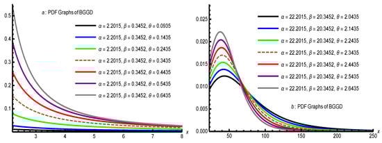  Figure 1. PDF graphs for different values of $\alpha ,\beta ,$ and $\theta$.

Theorem 1.

The probability density function (PDF) $f\left(y\right)$ of the BGGD distribution with CDF

$$\mathcal{F}\left(y\right)=1-{\displaystyle \frac{{\beta }^{\theta }}{{\left(\beta -1+{\left(\frac{y}{\alpha }\right)}^{\theta }\right)}^{\theta }}},y>\alpha ,\alpha ,\beta ,\theta >0,$$

can be derived by solving the generalized Burr-type differential equation:

$${\displaystyle \frac{f^{\prime }\left(y\right)}{f\left(y\right)}}={\displaystyle \frac{(\theta -1)(\beta -1)-(\theta \beta +1){\left(\frac{y}{\alpha }\right)}^{\theta }}{y\left(\beta -1+{\left(\frac{y}{\alpha }\right)}^{\theta }\right)}}.$$

Proof. 

In order to prove and derive the PDF of the above function, we start with ${\displaystyle \frac{1}{f\left(y\right)}}{\displaystyle \frac{df\left(y\right)}{dy}}={\displaystyle \frac{P\left(y\right)}{Q\left(y\right)}}$, where $P\left(y\right)$ and $Q\left(y\right)$ are continuous functions of y, $Q\left(y\right)\ne 0$, for any y, and $x=f\left(y\right)$ is the unknown function to be determined, whose specific value is y. The solution to this differential equation will lead to the PDF of the Generalized Three-Parameter Burr XII Distribution. To generate the Generalized Three-Parameter Burr XII Distribution, from ${\displaystyle \frac{1}{f\left(y\right)}}{\displaystyle \frac{df\left(y\right)}{dy}}={\displaystyle \frac{P\left(y\right)}{Q\left(y\right)}}$, we have ${\displaystyle \frac{f^{\prime }\left(y\right)}{fy}}={\displaystyle \frac{P\left(y\right)}{Q\left(y\right)}}$ or ${\displaystyle \frac{dlnf\left(y\right)}{dy}}={\displaystyle \frac{P\left(y\right)}{Q\left(y\right)}}$. By integrating both sides of ${\displaystyle \frac{dlnf\left(y\right)}{dy}}={\displaystyle \frac{P\left(y\right)}{Q\left(y\right)}}$ with respect to y, we obtain $lnf\left(y\right)=lnC+\int r\left(y\right)dy$ where $r\left(y\right)={\displaystyle \frac{P\left(y\right)}{Q\left(y\right)}}$. For getting $r\left(y\right)$ we proceed through the following steps: Let $z={\left({\displaystyle \frac{y}{\alpha }}\right)}^{\theta }$. The CDF becomes:

$$\mathcal{F}\left(y\right)=1-{\left(1+{\displaystyle \frac{z-1}{\beta }}\right)}^{-\theta }.$$

Differentiating the CDF with respect to y:

$$f\left(y\right)={\displaystyle \frac{d}{dy}}\left[1-{\left(1+{\displaystyle \frac{z-1}{\beta }}\right)}^{-\theta }\right]=\theta {\left(1+{\displaystyle \frac{z-1}{\beta }}\right)}^{-\theta -1}·{\displaystyle \frac{d}{dy}}\left({\displaystyle \frac{z-1}{\beta }}\right).$$

Since ${\displaystyle \frac{dz}{dy}}={\displaystyle \frac{\theta y^{\theta -1}}{{\alpha }^{\theta }}}$, we obtain:

$$f\left(y\right)={\displaystyle \frac{{\theta }^2{\beta }^{\theta }{y}^{\theta -1}}{{\alpha }^{\theta }{\left(\beta -1+{\left(\frac{y}{\alpha }\right)}^{\theta }\right)}^{\theta +1}}}.$$

Taking the natural logarithm of $f\left(y\right)$:

$$lnf\left(y\right)=ln\left({\theta }^2{\beta }^{\theta }\right)+(\theta -1)lny-\theta ln\alpha -(\theta +1)ln\left(\beta -1+{\left({\displaystyle \frac{y}{\alpha }}\right)}^{\theta }\right).$$

Differentiating with respect to y:

$${\displaystyle \frac{f^{\prime }\left(y\right)}{f\left(y\right)}}={\displaystyle \frac{\theta -1}{y}}-{\displaystyle \frac{(\theta +1)\theta {\left(\frac{y}{\alpha }\right)}^{\theta -1}\frac{1}{\alpha }}{\beta -1+{\left(\frac{y}{\alpha }\right)}^{\theta }}}={\displaystyle \frac{\theta -1}{y}}-{\displaystyle \frac{(\theta +1)\theta {\left(\frac{y}{\alpha }\right)}^{\theta }}{y\left(\beta -1+{\left(\frac{y}{\alpha }\right)}^{\theta }\right)}}.$$

(2)

Combining terms over a common denominator to rewrite in generalized Burr form as

$${\displaystyle \frac{f^{\prime }\left(y\right)}{f\left(y\right)}}={\displaystyle \frac{(\theta -1)\left(\beta -1+{\left(\frac{y}{\alpha }\right)}^{\theta }\right)-(\theta +1)\theta {\left(\frac{y}{\alpha }\right)}^{\theta }}{y\left(\beta -1+{\left(\frac{y}{\alpha }\right)}^{\theta }\right)}}.$$

Expanding the numerator:

$$(\theta -1)(\beta -1)+(\theta -1){\left({\displaystyle \frac{y}{\alpha }}\right)}^{\theta }-(\theta +1)\theta {\left({\displaystyle \frac{y}{\alpha }}\right)}^{\theta }=(\theta -1)(\beta -1)-({\theta }^2+1){\left({\displaystyle \frac{y}{\alpha }}\right)}^{\theta }.$$

Thus, we obtain the generalized Burr-type differential equation as

$${\displaystyle \frac{f^{\prime }\left(y\right)}{f\left(y\right)}}={\displaystyle \frac{(\theta -1)(\beta -1)-({\theta }^2+1){\left(\frac{y}{\alpha }\right)}^{\theta }}{y\left(\beta -1+{\left(\frac{y}{\alpha }\right)}^{\theta }\right)}}={\displaystyle \frac{P\left(y\right)}{Q\left(y\right)}},$$

(3)

on compared to the generalized Burr differential equation as expressed in Equation (4) with Equation (3)

$${\displaystyle \frac{f^{\prime }\left(y\right)}{f\left(y\right)}}={\displaystyle \frac{(c-1)-(ck+1){\left(\frac{b}{y}\right)}^c}{y\left[1+{\left(\frac{y}{b}\right)}^c\right]}},$$

(4)

Now integrating Equation (2) with respect to y we obtain

$$lnf\left(y\right)=(\theta -1)ln\left|y\right|-(1+\theta )ln\left|{\left({\displaystyle \frac{y}{\alpha }}\right)}^{\theta }+\beta -1\right|+C,\Rightarrow f\left(x\right)=C·y^{\theta -1}·{\left[{\left({\displaystyle \frac{y}{\alpha }}\right)}^{\theta }+\beta -1\right]}^{-(1+\theta )},$$

where C is the constant of integration. Please note that the BGGD is not a standard Burr XII distribution; however, its PDF does satisfy a generalized Burr-type differential equation with an additional offset parameter $\beta$. Therefore, we call it as Bounded Gamma–Gompertz Distribution (BGGD). Its survival function (SF) and probability density function (PDF) are defined as follows:

$$\mathcal{S}\left(y\right)={\displaystyle \frac{{\beta }^{\theta }}{{(\beta -1+{\left(\frac{y}{\alpha }\right)}^{\theta })}^{\theta }}},y>\alpha ,\alpha >0,\beta >0,\theta >0.$$

(5)

and

$$f(y;\alpha ,\beta ,\theta )={\displaystyle \frac{{\left(\frac{y}{\alpha }\right)}^{\theta }{\beta }^{\theta }{\left({\left(\frac{y}{\alpha }\right)}^{\theta }+\beta -1\right)}^{-1-\theta }{\theta }^2}{y}},y>\alpha ,\alpha >0,\beta >0,\theta >0,$$

(6)

where $\alpha >0$ is the scale parameter, $\beta >0$ and $\theta >0$ are shape parameters. Similarly, another important measure is the hazard function $\mathcal{H}\left(t\right)$ which represents the instantaneous rate of failure at time t, given that the subject has survived up to time t. Mathematically, it is defined as: $\mathcal{H}\left(t\right)={\displaystyle \frac{f\left(t\right)}{\mathcal{S}\left(t\right)}}$ and for BGGD it is expressed as

$$\mathcal{H}(y;\alpha ,\beta ,\theta )={\displaystyle \frac{{\left(\frac{y}{\alpha }\right)}^{\theta }{\left({\left(\frac{y}{\alpha }\right)}^{\theta }+\beta -1\right)}^{-1}{\theta }^2}{y}}.y>\alpha ,\alpha >0,\beta >0,\theta >0$$

(7)

□

2.2. PDF and HRF Shapes and Behavior

2.2.1. Mode of Distribution

The mode is found by solving ${\displaystyle \frac{d}{dy}}lnf\left(y\right)=0.$ Beginning with the logarithm of Equation (6)

$$lnf\left(y\right)=\theta ln\left(\beta \right)+\theta ln\left({\displaystyle \frac{y}{\alpha }}\right)-(\theta +1)ln\left(\beta -1+{\left({\displaystyle \frac{y}{\alpha }}\right)}^{\theta }\right)+2ln\left(\theta \right)-ln\left(y\right).$$

Differentiating with respect to y:

$${\displaystyle \frac{d}{dy}}lnf\left(y\right)={\displaystyle \frac{\theta }{y}}-{\displaystyle \frac{(\theta +1)}{\beta -1+{\left(\frac{y}{\alpha }\right)}^{\theta }}}·\theta {\displaystyle \frac{1}{\alpha }}{\left({\displaystyle \frac{y}{\alpha }}\right)}^{\theta -1}-{\displaystyle \frac{1}{y}}.$$

Simplify:

$${\displaystyle \frac{d}{dy}}lnf\left(y\right)={\displaystyle \frac{\theta -1}{y}}-{\displaystyle \frac{\theta (\theta +1)}{y}}·{\displaystyle \frac{{\left(\frac{y}{\alpha }\right)}^{\theta }}{\beta -1+{\left(\frac{y}{\alpha }\right)}^{\theta }}}.$$

Set the derivative to zero:

$${\displaystyle \frac{\theta -1}{y}}={\displaystyle \frac{\theta (\theta +1)}{y}}·{\displaystyle \frac{{\left(\frac{y}{\alpha }\right)}^{\theta }}{\beta -1+{\left(\frac{y}{\alpha }\right)}^{\theta }}}.$$

Multiply both sides by y (since $y>\alpha >0$) and let $u={\left({\displaystyle \frac{y}{\alpha }}\right)}^{\theta }$:

$$\theta -1=\theta (\theta +1)·{\displaystyle \frac{u}{\beta -1+u}}.$$

Solving for u:

$$\begin{array}{cc}\hfill (\theta -1)(\beta -1+u)& =\theta (\theta +1)u,\hfill \\ \hfill (\theta -1)(\beta -1)+(\theta -1)u& =\theta (\theta +1)u,\hfill \\ \hfill (\theta -1)(\beta -1)& =\left(\theta (\theta +1)-(\theta -1)\right)u\hfill \\ \hfill & =({\theta }^2+\theta -\theta +1)u\hfill \\ \hfill & =({\theta }^2+1)u.\hfill \end{array}$$

Thus,

$$u={\displaystyle \frac{(\theta -1)(\beta -1)}{{\theta }^2+1}}.$$

Substituting back $u={\left({\displaystyle \frac{y_m}{\alpha }}\right)}^{\theta }$, we find the mode:

$$y_m=\alpha {\left({\displaystyle \frac{(\theta -1)(\beta -1)}{{\theta }^2+1}}\right)}^{1/\theta }.$$

For $y_m$ to be greater than the lower bound $\alpha$, we require

$${\displaystyle \frac{(\theta -1)(\beta -1)}{{\theta }^2+1}}>0.$$

Given $\beta >0$ and ${\theta }^2+1>0$, this requires $(\theta -1)(\beta -1)>0$. If $\beta >1$, this simplifies to $\theta >1$. If $\theta \le 1$, the critical point $y_m\le \alpha$ lies outside the support. In this case, the derivative ${\displaystyle \frac{d}{dy}}lnf\left(y\right)$ can be shown to be negative for all $y>\alpha$, implying the PDF is strictly decreasing and its maximum is at the boundary $y\to {\alpha }^{+}$.

2.2.2. Development of Formal Theorems on PDF Log-Concavity and HRF Monotonicity

Here we shall prove the log-concavity of the PDF and the monotonicity of the HRF. We will build upon the provided expressions with the requirements.

2.2.3. Log-Concavity of the PDF

A function is log-concave if its logarithm is a concave function. This is a strong property with important implications for the unimodality and reliability of a distribution.

Theorem 2.

Let Y follow the BGGD with PDF $f(y;\alpha ,\beta ,\theta )$ as defined in Equation (11), for $y>\alpha$. The PDF $f\left(y\right)$ is log-concave if and only if $\theta \ge 1$.

Proof. 

We start with the log-PDF from Equation (6):

$$lnf\left(y\right)=\theta ln\left(\beta \right)+\theta ln\left({\displaystyle \frac{y}{\alpha }}\right)-(\theta +1)ln\left(\beta -1+{\left({\displaystyle \frac{y}{\alpha }}\right)}^{\theta }\right)+2ln\left(\theta \right)-ln\left(y\right).$$

(8)

To prove log-concavity, we need to show that the second derivative of $lnf\left(y\right)$ with respect to y is non-positive.

• Define $t={\left({\displaystyle \frac{y}{\alpha }}\right)}^{\theta }$. Then $y=\alpha t^{1/\theta }$. It simplifies analysis to work with t.
• First, compute the first derivative:

$${\displaystyle \frac{d}{dy}}lnf\left(y\right)={\displaystyle \frac{\theta }{y}}-{\displaystyle \frac{(\theta +1)}{\beta -1+t}}·{\displaystyle \frac{d}{dy}}t-{\displaystyle \frac{1}{y}}.$$

Since $t={(y/\alpha )}^{\theta }$, we have ${\displaystyle \frac{dt}{dy}}={\displaystyle \frac{\theta }{y}}t$. Thus,

$${\displaystyle \frac{d}{dy}}lnf\left(y\right)={\displaystyle \frac{\theta -1}{y}}-{\displaystyle \frac{\theta (\theta +1)}{y}}·{\displaystyle \frac{t}{\beta -1+t}}.$$

Substituting t:

$$g\left(t\right):={\displaystyle \frac{d}{dy}}lnf\left(y\right)={\displaystyle \frac{1}{\alpha t^{1/\theta }}}\left[\theta -1-{\displaystyle \frac{\theta (\theta +1)t}{\beta -1+t}}\right].$$

Differentiating $g\left(t\right)$ with respect to y:

$${\displaystyle \frac{d^2}{d{y}^2}}lnf\left(y\right)={\displaystyle \frac{dg}{dt}}·{\displaystyle \frac{dt}{dy}}.$$

Calculations show that:

$${\displaystyle \frac{d^2}{d{y}^2}}lnf\left(y\right)=-{\displaystyle \frac{\theta }{{\alpha }^2}}{t}^{-2/\theta }\left[{\displaystyle \frac{\theta -1}{\theta }}+{\displaystyle \frac{(\theta +1)t}{\beta -1+t}}+{\displaystyle \frac{\theta (\theta +1)(\beta -1)t}{{(\beta -1+t)}^2}}\right].$$

Denote

$$B\left(t\right):={\displaystyle \frac{\theta -1}{\theta }}+{\displaystyle \frac{(\theta +1)t}{\beta -1+t}}+{\displaystyle \frac{\theta (\theta +1)(\beta -1)t}{{(\beta -1+t)}^2}}.$$

The sign of the second derivative depends on $B\left(t\right)$. Since the prefactor is negative for $y>\alpha$, the sign of ${\displaystyle \frac{d^2}{d{y}^2}}lnf\left(y\right)$ is opposite to that of $B\left(t\right)$.

• - For $\theta \ge 1$:

$${\displaystyle \frac{\theta -1}{\theta }}\ge 0,$$

and the remaining terms are positive, so $B\left(t\right)>0$. Thus,

$${\displaystyle \frac{d^2}{d{y}^2}}lnf\left(y\right)<0,$$

establishing log-concavity.

• - For $\theta <1$:

$${\displaystyle \frac{\theta -1}{\theta }}<0,$$

and for y close to $\alpha$ (i.e., $t\to 1$), the negative term can dominate, making $B\left(t\right)<0$, and thus the second derivative positive, violating log-concavity.    □

Conclusion: $f\left(y\right)$ is log-concave if and only if $\theta \ge 1$.

2.3. Monotonicity of the Hazard Rate Function (HRF)

Let us define the hazard rate: $\mathcal{H}\left(y\right)={\displaystyle \frac{f\left(y\right)}{\mathcal{S}\left(y\right)}}$, where $\mathcal{S}\left(y\right)$ is the survival function. The next theorem studies the change points of the distribution.

Theorem 3.

Let $Y\sim BGGD(\alpha ,\beta ,\theta )$ with hazard rate function

$$\mathcal{H}(y;\alpha ,\beta ,\theta )={\displaystyle \frac{{\left(\frac{y}{\alpha }\right)}^{\theta }}{{\left({\left(\frac{y}{\alpha }\right)}^{\theta }+\beta -1\right)}^{-1}{\theta }^{2}y}},y>\alpha ,\alpha >0,\beta >0,\theta >0.$$

The behavior of $\mathcal{H}\left(y\right)$ is as follows:

• If $\beta \ge 1$, the hazard rate $\mathcal{H}\left(y\right)$ is strictly decreasing for all $y>\alpha$.
• If $\beta <1$, the hazard rate $H\left(y\right)$ has a unique mode (change point) at

$$y_c=\alpha {\left((1-\theta )(1-\beta )\right)}^{1/\theta },$$

provided $\theta <1$. In this case, $\mathcal{H}\left(y\right)$ is unimodal (increasing for $\alpha <y<y_c$ and decreasing for $y>y_c$).

Proof. 

We analyze the monotonicity of $\mathcal{H}\left(y\right)$ by examining the derivative of its logarithm.

• Start with the HRF:

$$\mathcal{H}\left(y\right)={\displaystyle \frac{{\theta }^2}{y}}·{\displaystyle \frac{{\left(\frac{y}{\alpha }\right)}^{\theta }}{{\left(\frac{y}{\alpha }\right)}^{\theta }+\beta -1}}.$$

Take the natural logarithm:

$$ln\mathcal{H}\left(y\right)=2ln\theta -lny+\theta ln\left({\displaystyle \frac{y}{\alpha }}\right)-ln\left({\left({\displaystyle \frac{y}{\alpha }}\right)}^{\theta }+\beta -1\right).$$

Differentiate with respect to y:

$${\displaystyle \frac{d}{dy}}ln\mathcal{H}\left(y\right)=-{\displaystyle \frac{1}{y}}+{\displaystyle \frac{\theta }{y}}-{\displaystyle \frac{1}{{\left(\frac{y}{\alpha }\right)}^{\theta }+\beta -1}}·{\displaystyle \frac{d}{dy}}\left[{\left({\displaystyle \frac{y}{\alpha }}\right)}^{\theta }\right].$$

Compute the derivative in the last term:

$${\displaystyle \frac{d}{dy}}\left[{\left({\displaystyle \frac{y}{\alpha }}\right)}^{\theta }\right]={\displaystyle \frac{\theta }{\alpha }}{\left({\displaystyle \frac{y}{\alpha }}\right)}^{\theta -1}={\displaystyle \frac{\theta }{y}}{\left({\displaystyle \frac{y}{\alpha }}\right)}^{\theta }.$$

Substitute back:

$${\displaystyle \frac{d}{dy}}ln\mathcal{H}\left(y\right)=-{\displaystyle \frac{1}{y}}+{\displaystyle \frac{\theta }{y}}-{\displaystyle \frac{1}{{\left(\frac{y}{\alpha }\right)}^{\theta }+\beta -1}}·{\displaystyle \frac{\theta }{y}}{\left({\displaystyle \frac{y}{\alpha }}\right)}^{\theta }.$$

Simplify the first two terms: $-{\displaystyle \frac{1}{y}}+{\displaystyle \frac{\theta }{y}}={\displaystyle \frac{\theta -1}{y}}$. Thus,

$${\displaystyle \frac{d}{dy}}lnH\left(y\right)={\displaystyle \frac{\theta -1}{y}}-{\displaystyle \frac{\theta }{y}}·{\displaystyle \frac{{\left(\frac{y}{\alpha }\right)}^{\theta }}{{\left(\frac{y}{\alpha }\right)}^{\theta }+\beta -1}}.$$

(9)

On equating Equation (9) to zero, we obtain the mode of the hazard function as:

$$y_c=\alpha {\left((\theta -1)(\beta -1)\right)}^{1/\theta }.$$

For this to be valid, we need $y_c>\alpha$, which requires $(\theta -1)(\beta -1)>1$. Since $\theta -1>0$ and $\beta -1>0$, this is a condition on the parameters. If $(\theta -1)(\beta -1)\le 1$, the critical point $y_c\le \alpha$, which is outside the support.    □

Now the cumulative hazard function is defined as $\mathsf{\Lambda }\left(y\right):=-ln\mathcal{S}\left(y\right),$ has derivatives related to $\mathcal{H}\left(y\right)$: $\mathcal{H}\left(y\right)={\displaystyle \frac{d}{dy}}\mathsf{\Lambda }\left(y\right).$

Theorem 4.

The HRF $\mathcal{H}\left(y\right)$ is decreasing for all $y>\alpha$ if $\beta \ge 1$. If $\beta <1$, the HRF may be non-monotonic, potentially exhibiting an upside-down bathtub shape.

Proof. 

The survival function:

$$\mathcal{S}\left(y\right)={\displaystyle \frac{{\beta }^{\theta }}{{\left(\beta -1+{\left(\frac{y}{\alpha }\right)}^{\theta }\right)}^{\theta }}}.$$

The cumulative hazard:

$$\mathsf{\Lambda }\left(y\right)=-\theta ln\beta +\theta ln\left(\beta -1+{\left({\displaystyle \frac{y}{\alpha }}\right)}^{\theta }\right).$$

Differentiating:

$$\mathcal{H}\left(y\right)={\displaystyle \frac{d}{dy}}\mathsf{\Lambda }\left(y\right)={\displaystyle \frac{\theta }{\beta -1+t}}·{\displaystyle \frac{dt}{dy}}={\displaystyle \frac{{\theta }^{2}t}{y(\beta -1+t)}},$$

where $t={(y/\alpha )}^{\theta }.$

• Differentiating $\mathcal{H}\left(y\right)$:

$${\displaystyle \frac{d}{dy}}\mathcal{H}\left(y\right)={\displaystyle \frac{{\theta }^3}{{\alpha }^2}}·{\displaystyle \frac{1}{{(\beta -1+t)}^2}}·D\left(t\right),$$

where

$$D\left(t\right)=\left(1-{\displaystyle \frac{1}{\theta }}\right)(\beta -1)-{\displaystyle \frac{1}{\theta }}t.$$

- When $\beta \ge 1$: $(\beta -1)\ge 0,$ so $D\left(t\right)\le 0$ for all $t>1$. Therefore,

$${\displaystyle \frac{d}{dy}}\mathcal{H}\left(y\right)<0,$$

and the HRF is decreasing.

• - When $\beta <1$: $D\left(t\right)$ is linear in t with a negative slope, possibly crossing zero at

$$t_c=\theta (\beta -1)(1-{\displaystyle \frac{1}{\theta }})=(\theta -1)(1-\beta ).$$

If $t_c>1$, $D\left(t\right)>0$ for $t<t_c$, implying the HRF initially increases and then decreases, exhibiting a non-monotonic shape.

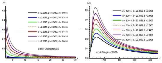
Conclusion: The HRF is decreasing for $\beta \ge 1$, and may be non-monotonic when $\beta <1$. These theorems establish a rigorous foundation for the distribution’s shape properties, replacing heuristic observations with formal proofs. Moreover, the Figure 2 portrays that as parameters increase, the hazard functions tend to decrease more gradually, indicating a heavier tail and increased spread. Conversely, smaller parameters produce sharper declines, reflecting lighter tails and less dispersion. These behaviors highlight the sensitivity of the hazard functions to parameter changes.    □

Figure 2. Some HRF of BGGD for different values of parameters.

2.4. Log-Concavity and Curvature Analysis

Log-concavity plays a significant role in statistics, optimization, and economics because it ensures nice properties like unimodality, stability under convolution, and convexity of the negative log-likelihood, which facilitates efficient estimation and inference.

2.4.1. Log-Concavity of the BGGD

Let Y $\sim \mathrm{BGGD}(\alpha ,\beta ,\theta )$ while its PDF ith lograthmic form is expressed in Equation (8) To test for log-concavity, we examine the second derivative of $lnf\left(y\right)$:

$${\displaystyle \frac{d^2}{d{y}^2}}lnf\left(y\right)=\underset{\mathrm{Negative}\mathrm{for}\theta >1}{\underbrace{-{\displaystyle \frac{\theta -1}{y^2}}}}+\underset{\mathrm{Positive}}{\underbrace{{\displaystyle \frac{\theta (\theta +1){\left(\frac{y}{\alpha }\right)}^{\theta -2}}{{\alpha }^2{\left(\beta -1+{\left(\frac{y}{\alpha }\right)}^{\theta }\right)}^2}}}},$$

from we can conclude that for $\theta <1$, the PDF is not log-concave (first term dominates), while for $\theta \ge 1$, log-concavity depends on the balance between terms (see Theorem 2).

2.4.2. Second Derivative of the PDF

The second derivative $f^{″}\left(y\right)$ is complex but can be expressed as:

$$f^{″}(y)=f(y)\left[\left({\displaystyle \frac{(\theta -1)(\theta -2)}{y^2}}-{\displaystyle \frac{2\theta ({\theta }^2-1){\left(\frac{y}{\alpha }\right)}^{\theta -1}}{\alpha y(\beta -1+{\left(\frac{y}{\alpha }\right)}^{\theta })}}+{\displaystyle \frac{{\theta }^2(\theta +1){\left(\frac{y}{\alpha }\right)}^{2\theta -2}}{{\alpha }^2{\left(\beta -1+{\left(\frac{y}{\alpha }\right)}^{\theta }\right)}^2}}\right)\right].$$

It implies that for $\theta <1$, $f^{″}\left(y\right)$ may change sign (possible inflection points) and for $\theta \ge 2$, the PDF is more likely to be unimodal and smooth.

2.4.3. Hazard Rate Function (HRF) Analysis

From Equation (7) we computed the second derivative of $ln\mathcal{H}\left(y\right)$:

$${\displaystyle \frac{d^2}{d{y}^2}}ln\mathcal{H}\left(y\right)=-{\displaystyle \frac{1}{y^2}}-{\displaystyle \frac{\theta (\beta -1){\left(\frac{y}{\alpha }\right)}^{\theta -2}}{{\alpha }^2{\left({\left(\frac{y}{\alpha }\right)}^{\theta }+\beta -1\right)}^2}}.$$

It is observed that (${\displaystyle \frac{d^2}{d{y}^2}}ln\mathcal{H}\left(y\right)<0$), confirming that $\mathcal{H}\left(y\right)$ is log-concave for all parameter values. Likewise, the second derivative of HRF i.e., ${\mathcal{H}}^{″}\left(y\right)$ is:

$${\mathcal{H}}^{″}(y)={\displaystyle \frac{{\theta }^2{\left(\frac{y}{\alpha }\right)}^{\theta }\left[(\theta -1)(\theta -2){\left({\left(\frac{y}{\alpha }\right)}^{\theta }+\beta -1\right)}^2-2\theta (\theta +1)(\beta -1){\left(\frac{y}{\alpha }\right)}^{\theta }+{\theta }^2{(\beta -1)}^2\right]}{y^3{\alpha }^2{\left({\left(\frac{y}{\alpha }\right)}^{\theta }+\beta -1\right)}^3}}.$$

Its behavior for $\beta =1$, simplifies to ${\mathcal{H}}^{″}(y)={\displaystyle \frac{{\theta }^2(\theta -1)(\theta -2)}{y^3}}$, which changes sign at $\theta =1$ and $\theta =2$, for $\beta \ne 1$, the curvature depends on the interplay between $\theta$ and $\beta$. We conclude that PDF is Log-Concave if $\theta \ge 1$ (see Theorem 2) and its curvature can have inflection points. Similarly, HRF is Log-Concave for all $\theta ,\beta$ and its curvature for $\beta =1$ depends on $\theta$.

2.4.4. Rigorous Implications for Estimation and Modeling

Log-concavity has profound practical consequences:

• Maximum-Likelihood Estimation (MLE):

  -

  If PDF is log-concave ($\theta \ge 1$), $-lnf\left(y\right)$ is convex ⇒ the negative log-likelihood is convex in parameters ⇒ unique global maximum, no local optima.

  -

  Numerical optimization (Newton-Raphson, quasi-Newton) converges globally and rapidly.

  -

  Standard errors via observed Hessian are reliable.

• Shape-Constrained Inference:

  -

  Log-concave densities form a convex nonparametric class. BGGD with $\theta \ge 1$ can serve as a parametric anchor in shape-constrained estimation.

  -

  Enables confidence bands and hypothesis tests with known asymptotic behavior.

• Stability and Robustness:

  -

  Convolution of log-concave densities is log-concave ⇒ BGGD priors lead to log-concave posteriors under suitable likelihoods.

  -

  Useful in Bayesian modeling with heavy-tailed data (e.g., insurance, finance).

• Hazard Rate Modeling (Survival Analysis):

  -

  Log-concave HRF ⇒ log-concave survival function and increasing failure rate on average (IFRA) in some cases.

  -

  Implies aging properties: systems wear out predictably.

  -

  Facilitates nonparametric monotone hazard estimation with BGGD as a parametric benchmark.

• Practical Recommendation:

  -

  Use $\theta \ge 1$ for reliable MLE, interpretable shapes, and theoretical guarantees.

  -

  Use $\theta <1$ only with caution: expect multiple modes, optimization traps, and non-concave likelihoods.

  -

  Leverage log-concave HRF for robust survival modeling even when PDF is not log-concave.

3. Comparative Analysis of Bounded Probability Distributions

This section provides the Cumulative Distribution Functions (CDFs) for the BGGD and other competing bounded distributions. The CDF, $F\left(x\right)$, gives the probability that a random variable X takes a value less than or equal to x.

• Key Observations:

-

The BGGD and Kumaraswamy distributions possess a closed-form CDF, which is advantageous for direct probability calculations.

-

The Beta distribution’s CDF relies on the incomplete Beta function $I_x(a,b)$, which must be evaluated numerically and lacks a closed-form expression.

-

The Bounded Lomax has the simplest CDF form, which is a special case of the Kumaraswamy CDF when the shape parameter $a=1$.

• The BGGD represents a specialized three-parameter model that occupies a unique niche within the family of bounded distributions. When compared to established models like the Beta, Kumaraswamy, and Bounded Lomax distributions, the BGGD’s distinctive characteristics become apparent across multiple dimensions, including mathematical structure, hazard behavior, and practical applicability.

3.1. Mathematical Form and Flexibility

The BGGD is a three-parameter distribution $(\alpha ,\beta ,\theta )$ defined on $(\alpha ,\infty )$, with a complex probability density function incorporating power-law behavior. This formulation offers substantial flexibility for modeling heavy-tailed phenomena, albeit at the expense of mathematical simplicity. In comparison, the Beta distribution is the standard choice for modeling variables bounded in $(0,1)$, using its two-parameter form with Beta functions to accommodate diverse shapes, including U-shaped, J-shaped, reverse J-shaped, and unimodal densities. The Kumaraswamy distribution serves as a mathematically tractable two-parameter alternative to the Beta, providing closed-form expressions for both the CDF and quantile function while retaining similar shape versatility. Finally, the Bounded Lomax distribution is the most parsimonious option, typically using one or two parameters to model heavy tails via a simpler power-law structure derived from the Lomax distribution.

3.2. Hazard Function Characteristics

The behavior of the hazard function highlights key differences among these distributions. The BGGD exhibits a distinctive profile, starting at infinity at the lower bound and approaching a finite constant $({\theta }^2/\beta )$ at the upper bound, making it ideal for reliability studies with stabilizing risk over time. The Beta distribution provides highly flexible hazard shapes, including increasing, decreasing, bathtub, and inverted bathtub patterns, depending on its parameters. In contrast, the Kumaraswamy distribution always yields infinite hazard at the upper bound, limiting its use for long-term risk assessment. Similarly, the Bounded Lomax distribution has a strictly increasing hazard diverging to infinity at the upper bound, suitable for simple wear-out failures but less appropriate for complex hazard dynamics.

3.3. Statistical Practicality and Implementation

From an implementation perspective, the distributions vary significantly in their practical utility. The BGGD presents considerable challenges for parameter estimation due to its three-parameter structure and complex likelihood surfaces, requiring careful implementation and substantial sample sizes. The Beta distribution, while lacking closed-form CDF and quantile functions, benefits from well-established estimation procedures and extensive software support. The Kumaraswamy distribution excels in computational efficiency with its closed-form expressions, making it ideal for simulation studies and applications requiring frequent quantile calculations. The Bounded Lomax offers the simplest implementation with straightforward parameter estimation and interpretation, though at the cost of limited shape flexibility.

3.4. Domain Applications and Selection Guidelines

The choice among these distributions depends fundamentally on the modeling context and requirements. The BGGD proves most valuable for heavy-tailed bounded data where finite long-term hazard is theoretically justified, such as in certain reliability engineering, insurance claim modeling, and income distribution applications. The Beta distribution remains the optimal choice for general proportion modeling, Bayesian analysis, and applications demanding maximum shape flexibility. The Kumaraswamy distribution serves as an excellent practical alternative when closed-form solutions and computational efficiency are priorities, particularly in hydrological studies and simulation-heavy applications. The Bounded Lomax provides the best option for simple heavy-tailed bounded phenomena where interpretability and parsimony outweigh the need for sophisticated shape flexibility.

In conclusion, while the BGGD introduces valuable specialized capabilities for heavy-tailed bounded modeling with finite hazard limits, its adoption should be justified by demonstrated superior fit compared to more established alternatives. The Beta distribution maintains its position as the most versatile general-purpose bounded model, with Kumaraswamy offering superior tractability for many practical applications, and Bounded Lomax providing a straightforward solution for simple heavy-tailed scenarios. The selection among these distributions ultimately hinges on the specific balance required between mathematical sophistication, implementation practicality, and theoretical appropriateness for the phenomenon under investigation.

3.5. Moments and Moment Generating Function (MGF)

Here, we will calculate the expressions for the moments and the moment generating function of the distribution that are important in any statistical analysis, especially in applied work. It is known that some of the most important characteristics of a distribution can be studied through its moments (for example, tendency, dispersion, skewness, and kurtosis).

Theorem 5.

Let $Y\sim BGGD(\alpha ,\beta ,\theta )$ with probability density function (PDF) given by

$$f(y;\alpha ,\beta ,\theta )={\displaystyle \frac{{\left(\frac{y}{\alpha }\right)}^{\theta }{\beta }^{\theta }{\left({\left(\frac{y}{\alpha }\right)}^{\theta }+\beta -1\right)}^{-1-\theta }{\theta }^2}{y}},y>\alpha ,\alpha >0,\beta >0,\theta >0.$$

1. 

The r-th raw moment, $\mathbb{E}\left[Y^r\right]$, exists and is given by

$$\mathbb{E}\left[Y^r\right]=\theta {\beta }^{\theta }{\alpha }^r{(\beta -1)}^{{\displaystyle \frac{r}{\theta }}-\theta }\mathbb{B}\left({\displaystyle \frac{1}{\beta }};{\displaystyle \frac{r}{\theta }}+1,\theta -{\displaystyle \frac{r}{\theta }}\right),$$

if and only if the following parameter conditions hold:

(a) 

$\beta >1$

(b) 

$r<{\theta }^2$

Here, $\mathbb{B}(z;a,b)={\int }_0^z{t}^{a-1}{(1-t)}^{b-1}dt$ is the incomplete Beta function.

2. 

The Moment Generating Function (MGF), $M_Y\left(t\right)=\mathbb{E}\left[e^{tY}\right]$, exists and is given by the series expansion

$$M_Y\left(t\right)=\theta {\beta }^{\theta }\sum _{k=0}^{\infty }{\displaystyle \frac{{\left(t\alpha \right)}^k}{k!}}{(\beta -1)}^{{\displaystyle \frac{k}{\theta }}-\theta }\mathbb{B}\left({\displaystyle \frac{1}{\beta }};{\displaystyle \frac{k}{\theta }}+1,\theta -{\displaystyle \frac{k}{\theta }}\right),$$

which converges for all $t\in \mathbb{R}$  under the same conditions $\beta >1$ and $\theta >0$.

Proof. 

By definition, the r-th raw moment is

$$\mathbb{E}\left[Y^r\right]={\int }_{\alpha }^{\infty }{y}^{r}f\left(y\right)dy.$$

Substituting the PDF $f\left(y\right)$:

$$\mathbb{E}\left[Y^r\right]={\int }_{\alpha }^{\infty }{y}^r·{\displaystyle \frac{{\left(\frac{y}{\alpha }\right)}^{\theta }{\beta }^{\theta }{\left({\left(\frac{y}{\alpha }\right)}^{\theta }+\beta -1\right)}^{-1-\theta }{\theta }^2}{y}}dy={\displaystyle \frac{{\theta }^2{\beta }^{\theta }}{{\alpha }^{\theta }}}{\int }_{\alpha }^{\infty }{\displaystyle \frac{y^{\theta +r-1}}{{\left[\beta -1+{\left(\frac{y}{\alpha }\right)}^{\theta }\right]}^{\theta +1}}}dy.$$

To evaluate this integral, we employ the substitution:

$$u={\left({\displaystyle \frac{y}{\alpha }}\right)}^{\theta }\Rightarrow y=\alpha u^{1/\theta },dy={\displaystyle \frac{\alpha }{\theta }}{u}^{{\displaystyle \frac{1}{\theta }}-1}du.$$

The limits change as follows: when $y=\alpha$, $u=1$; when $y\to \infty$, $u\to \infty .$

• Substituting into the integral:

$$\mathbb{E}\left[Y^r\right]={\displaystyle \frac{{\theta }^2{\beta }^{\theta }}{{\alpha }^{\theta }}}{\int }_1^{\infty }{\displaystyle \frac{{\left(\alpha u^{1/\theta }\right)}^{\theta +r-1}}{{\left[\beta -1+u\right]}^{\theta +1}}}·{\displaystyle \frac{\alpha }{\theta }}{u}^{{\displaystyle \frac{1}{\theta }}-1}du.$$

Simplifying the powers:

-

${\left(\alpha u^{1/\theta }\right)}^{\theta +r-1}={\alpha }^{\theta +r-1}{u}^{1+{\displaystyle \frac{r-1}{\theta }}}$

-

Multiplying by $u^{{\displaystyle \frac{1}{\theta }}-1}$ gives $u^{1+{\displaystyle \frac{r-1}{\theta }}+{\displaystyle \frac{1}{\theta }}-1}=u^{r/\theta }$

-

The constants: ${\displaystyle \frac{{\theta }^2{\beta }^{\theta }}{{\alpha }^{\theta }}}·{\alpha }^{\theta +r-1}·{\displaystyle \frac{\alpha }{\theta }}=\theta {\beta }^{\theta }{\alpha }^r$

• Thus, the moment simplifies elegantly to:

$$\mathbb{E}\left[Y^r\right]=\theta {\beta }^{\theta }{\alpha }^r{\int }_1^{\infty }{\displaystyle \frac{u^{r/\theta }}{{(\beta -1+u)}^{\theta +1}}}du.$$

(10)

We now focus on the integral $I={\int }_1^{\infty }{\displaystyle \frac{u^{a-1}}{{(b+u)}^c}}du$, where $a={\displaystyle \frac{r}{\theta }}+1$, $b=\beta -1$, and $c=\theta +1.$

• Let $u=bt\Rightarrow du=bdt$. The limits become: $u=1\Rightarrow t=1/b$, and $u\to \infty \Rightarrow t\to \infty$.

$$I={\int }_{1/b}^{\infty }{\displaystyle \frac{{\left(bt\right)}^{a-1}}{{(b+bt)}^c}}bdt=b^{a-1}b·b^{-c}{\int }_{1/b}^{\infty }{\displaystyle \frac{t^{a-1}}{{(1+t)}^c}}dt=b^{a-c}{\int }_{1/b}^{\infty }{\displaystyle \frac{t^{a-1}}{{(1+t)}^c}}dt.$$

We now use a standard integral identity, see [19]:

$${\int }_u^{\infty }{\displaystyle \frac{t^{\nu -1}dt}{{(1+t)}^{\mu +\nu }}}=\mathbb{B}\left({\displaystyle \frac{u}{1+u}};\nu ,\mu \right),[\mathrm{for}\mu >0,\nu >0,0\le u<\infty ].$$

Matching this to our integral, we have:

-

$\nu =a$

-

$\mu +\nu =c\Rightarrow \mu =c-a$

-

$u=1/b$

• Therefore,

$${\int }_{1/b}^{\infty }{\displaystyle \frac{t^{a-1}}{{(1+t)}^c}}dt=\mathrm{B}\left({\displaystyle \frac{1/b}{1+1/b}};a,c-a\right)=\mathbb{B}\left({\displaystyle \frac{1}{1+b}};a,c-a\right).$$

Substituting $b=\beta -1$, we obtain ${\displaystyle \frac{1}{1+b}}={\displaystyle \frac{1}{\beta }}.$

• Now, substituting back $a={\displaystyle \frac{r}{\theta }}+1$ and $c=\theta +1$:

$$c-a=(\theta +1)-\left({\displaystyle \frac{r}{\theta }}+1\right)=\theta -{\displaystyle \frac{r}{\theta }}.$$

Also, $b^{a-c}={(\beta -1)}^{\left({\displaystyle \frac{r}{\theta }}+1\right)-(\theta +1)}={(\beta -1)}^{{\displaystyle \frac{r}{\theta }}-\theta .}$

• Thus, the integral I becomes:

$$I={(\beta -1)}^{{\displaystyle \frac{r}{\theta }}-\theta }\mathbb{B}\left({\displaystyle \frac{1}{\beta }};{\displaystyle \frac{r}{\theta }}+1,\theta -{\displaystyle \frac{r}{\theta }}\right).$$

Substituting this result back into Equation (10):

$$\mathbb{E}\left[Y^r\right]=\theta {\beta }^{\theta }{\alpha }^r{(\beta -1)}^{{\displaystyle \frac{r}{\theta }}-\theta }\mathbb{B}\left({\displaystyle \frac{1}{\beta }};{\displaystyle \frac{r}{\theta }}+1,\theta -{\displaystyle \frac{r}{\theta }}\right).\hspace{1em}\square \hspace{1em}$$

The derivation is valid only if the integral converges and the arguments of the Beta function are positive.

1.

Condition $\beta >1$: This ensures $b=\beta -1>0$, which is crucial for the substitution $u=bt$ and for the power ${(\beta -1)}^{{\displaystyle \frac{r}{\theta }}-\theta }$ to be well-defined for all real r. If $\beta \le 1$, the term $\beta -1$ in the original PDF’s denominator becomes problematic for convergence near $y=\alpha$.

2.

Condition $r<{\theta }^2$: The incomplete Beta function $\mathrm{B}(z;p,q)$ requires its second and third arguments to be positive for the integral representation to be valid and finite.

-

The second argument is ${\displaystyle \frac{r}{\theta }}+1>0$, which is always true since $r\ge 0$ and $\theta >0$.

-

The critical condition comes from the third argument: $\theta -{\displaystyle \frac{r}{\theta }}>0$. Multiplying both sides by $\theta$ gives ${\theta }^2-r>0$, or equivalently, $r<{\theta }^2$.

• This condition, $r<{\theta }^2$, reveals that the BGGD possesses power-law tails. The distribution has finite moments only up to a certain order determined by its shape parameter $\theta$. Moments of order $r\ge {\theta }^2$ do not exist. This is a characteristic feature of heavy-tailed distributions. Now, we prove Theorem 5 (Part 2), that is, the “Derivation of the Moment Generating Function (MGF)”, as follows:
• The MGF is defined as $M_Y\left(t\right)=\mathbb{E}\left[e^{tY}\right]={\int }_{\alpha }^{\infty }{e}^{ty}f\left(y\right)dy$.
• Substituting the PDF and using the same substitution $u={(y/\alpha )}^{\theta }$ as before, we obtain:

$$M_Y\left(t\right)=\theta {\beta }^{\theta }{\int }_1^{\infty }{\displaystyle \frac{e^{t\alpha u^{1/\theta }}}{{(\beta -1+u)}^{\theta +1}}}du.$$

(11)

The exponential function can be expressed as its Maclaurin series, $e^{t\alpha u^{1/\theta }}={\sum }_{k=0}^{\infty }{\displaystyle \frac{{\left(t\alpha u^{1/\theta }\right)}^k}{k!}}={\sum }_{k=0}^{\infty }{\displaystyle \frac{{\left(t\alpha \right)}^k}{k!}}{u}^{k/\theta }$, which converges absolutely for all t and u.

• Substituting the series into the integral:

$$M_Y\left(t\right)=\theta {\beta }^{\theta }\sum _{k=0}^{\infty }{\displaystyle \frac{{\left(t\alpha \right)}^k}{k!}}{\int }_1^{\infty }{\displaystyle \frac{u^{k/\theta }}{{(\beta -1+u)}^{\theta +1}}}du.$$

The integral inside the sum is identical in form to the one solved for the raw moments in Part 1, with r replaced by k. Therefore, applying the same result:

$${\int }_1^{\infty }{\displaystyle \frac{u^{k/\theta }}{{(\beta -1+u)}^{\theta +1}}}du={(\beta -1)}^{{\displaystyle \frac{k}{\theta }}-\theta }\mathrm{B}\left({\displaystyle \frac{1}{\beta }};{\displaystyle \frac{k}{\theta }}+1,\theta -{\displaystyle \frac{k}{\theta }}\right).$$

Thus, the MGF is given by:

$$M_Y\left(t\right)=\theta {\beta }^{\theta }\sum _{k=0}^{\infty }{\displaystyle \frac{{\left(t\alpha \right)}^k}{k!}}{(\beta -1)}^{{\displaystyle \frac{k}{\theta }}-\theta }\mathrm{B}\left({\displaystyle \frac{1}{\beta }};{\displaystyle \frac{k}{\theta }}+1,\theta -{\displaystyle \frac{k}{\theta }}\right).$$

Convergence of the MGF Series: For any fixed $t\in \mathbb{R}$, the series converges because the k-th term is proportional to ${\displaystyle \frac{{\left|t\right|}^k}{k!}}$, and the factorial dominance in the denominator ensures convergence. The conditions $\beta >1$ and $\theta >0$ guarantee that each term in the series is well-defined. The condition $k<{\theta }^2$ from Part 2 is automatically satisfied for all k in the infinite sum for any fixed $\theta$, because the Gamma function in the asymptotic form of the Beta function for large k is suppressed by the factorial term $1/k!$.    □

Table 1 summarizes the results across 31 cases, each characterized by parameters $\alpha$, $\beta$, and $\theta$, along with their corresponding mean, standard deviation, skewness, and kurtosis. The parameter $\alpha$ varies broadly from 0.2 to 16.0, indicating diverse distribution shapes, while $\beta$ ranges from 0.5 to 45.0, reflecting different scale or location parameters. The mean values span from approximately 0.1831 (Case 3) to 1.7265 (Case 31), with standard deviations indicating varying degrees of dispersion among the cases. Skewness values range from negative to positive, with some distributions exhibiting left-tailed asymmetry (e.g., Case 1 with −0.5795) and others right-tailed (e.g., Case 32 with 1.7265). Kurtosis also varies, with some cases showing lighter tails (negative kurtosis) and others heavier tails (positive kurtosis), such as Case 32 with 1.2042. Overall, the data reflect a wide diversity of distributional behaviors, from symmetric to highly skewed and heavy-tailed distributions.

Table 1. Descriptive summary of BGGD distribution.

Case	$\mathit{\alpha }$	$\mathit{\beta }$	$\mathit{\theta }$	Mean	Standard Deviation	Skewness	Kurtosis
1	1.0	4.0	2.3	0.5969	0.2710	−0.5795	−0.4788
2	1.0	5.0	2.5	0.4979	0.3472	−0.3126	−1.3476
3	0.5	6.0	2.9	0.2452	0.1831	−0.2824	−1.4919
4	1.0	10.0	3.3	0.3094	0.3865	0.5900	−1.4388
5	1.0	8.0	3.7	0.4838	0.3908	−0.2342	−1.6571
6	0.8	7.0	4.3	0.5835	0.1950	−1.5920	2.3293
7	1.0	12.0	4.7	0.4065	0.4166	0.1514	−1.8198
8	3.0	6.0	3.5	1.9734	0.8645	−1.1200	0.3445
9	1.0	20.0	5.6	0.2784	0.4017	0.8112	−1.2374
10	1.0	15.0	6.0	0.4312	0.4303	0.0684	−1.8792
11	2.0	8.0	3.5	0.8911	0.7874	−0.0621	−1.7265
12	1.0	30.0	8.0	0.2744	0.4119	0.8691	−1.1823
13	2.0	10.0	3.5	0.6727	0.7888	0.4565	−1.5867
14	1.5	4.5	2.4	0.8103	0.4812	−0.4811	−1.0069
15	0.7	7.5	2.8	0.2435	0.2673	0.3815	−1.5776
16	1.0	9.0	4.0	0.4653	0.4009	−0.1393	−1.7425
17	0.9	11.0	5.0	0.4457	0.3708	−0.2492	−1.7489
18	2.5	5.5	3.5	1.8649	0.4008	0.3910	−5.8379
19	1.0	25.0	6.0	0.2352	0.3854	1.0809	−0.7352
20	1.2	14.0	7.0	0.6994	0.4935	−0.6188	−1.4575
21	3.0	7.0	3.5	1.5945	1.1109	−0.4680	−1.3841
22	1.0	18.0	8.0	0.5074	0.4392	−0.2351	−1.8531
23	0.6	22.0	9.0	0.2773	0.2695	−0.0179	−1.9340
24	1.0	28.0	10.0	0.3949	0.4504	0.2915	−1.8670
25	2.0	12.0	3.5	0.5400	0.7582	0.8137	−1.1451
26	1.5	16.0	3.5	0.2902	0.5166	1.3325	−0.0227
27	1.0	35.0	12.0	0.3811	0.4540	0.3716	−1.8271
28	3.0	9.0	3.5	1.1502	1.1938	0.2278	−1.7235
29	1.0	40.0	13.0	0.3595	0.4519	0.4778	−1.7419
30	1.0	45.0	14.0	0.3431	0.4496	0.5616	−1.6586
31	2.0	20.0	3.5	0.3014	0.6299	1.7265	1.2042

3.6. Quantile Function

The quantile function $Q\left(p\right)$ for the given distribution can be derived by inverting the cumulative distribution function $\mathcal{F}\left(y\right)=1-{\beta }^{\theta }/{\left(\beta -1+{(y/\alpha )}^{\theta }\right)}^{\theta }$. Starting from $p=1-{\beta }^{\theta }/{\left(\beta -1+{(y/\alpha )}^{\theta }\right)}^{\theta }$, we first isolate the denominator to obtain $1-p={\beta }^{\theta }/{\left(\beta -1+{(y/\alpha )}^{\theta }\right)}^{\theta }$. Taking reciprocals yields ${\left(\beta -1+{(y/\alpha )}^{\theta }\right)}^{\theta }/{\beta }^{\theta }=1/(1-p)$. Raising both sides to the $1/\theta$ power gives $\left(\beta -1+{(y/\alpha )}^{\theta }\right)/\beta ={(1-p)}^{-1/\theta }$. Solving for ${(y/\alpha )}^{\theta }$ produces ${(y/\alpha )}^{\theta }=\beta \left[{(1-p)}^{-1/\theta }-1\right]+1$, which leads to the final quantile function $Q\left(p\right)=\alpha {\left[\beta \left({(1-p)}^{-1/\theta }-1\right)+1\right]}^{1/\theta }$ for $0<p<1$. This function properly recovers the boundary conditions, approaching $\alpha$ as $p\to 0^{+}$ and diverging to infinity as $p\to 1^{-}$. Two important special cases emerge: when $\beta =1$, the quantile function reduces to a Pareto-type form $Q\left(p\right)=\alpha {(1-p)}^{-1/{\theta }^2}$, while for $\theta =1$ it simplifies to a shifted Lomax distribution $Q\left(p\right)=\alpha \left(1+\beta p/(1-p)\right)$. The derived quantile function enables Monte Carlo simulation through inverse transform sampling and facilitates risk assessment through the calculation of extreme quantiles.

4. Tail-Risk Evaluation

Tail-risk management focuses on identifying and reducing the impact of rare but severe financial losses that occur in the extreme ends (tails) of probability distributions. It uses tools like mean residual life or life expectancy (MRL), Value at Risk (VaR), Tail Value at Risk (TVaR), and Expected Shortfall (ES) to measure and assess these risks. Strategies such as stress testing, scenario analysis, diversification, and financial instruments like options and insurance help mitigate these risks. Managing tail risk is crucial to safeguarding capital and maintaining financial stability during crises or market shocks.

4.1. Mean Residual Life (MRL)

The mean residual life (MRL) or life expectancy is an important characteristic of the model. It is useful in reliability analysis of mechanical systems, survival analysis in medical studies, and risk assessment in financial modeling. It represents the expected additional lifetime given survival until time t. For a continuous random variable Y with survival function $\mathcal{S}\left(y\right)=1-\mathcal{F}\left(y\right)$ MRL is given by:

$$\mathrm{MRL}\left(t\right)=\mathbb{E}[Y-t\mid Y>t]={\displaystyle \frac{1}{\mathcal{S}\left(t\right)}}{\int }_t^{\infty }\mathcal{S}\left(t\right)dt.$$

(12)

Now on incorporating the survival function of BGGD ($\alpha ,\beta ,\theta$) as given in Equation (5) into Equation (12), making the substitution $u={\left({\displaystyle \frac{t}{\alpha }}\right)}^{\theta }$, $dt={\displaystyle \frac{\alpha }{\theta }}{u}^{{\displaystyle \frac{1}{\theta }}-1}du$ and using the integral

$${\int }_x^{\infty }{\displaystyle \frac{t^{a-1}}{{(1+t)}^c}}dt={\mathbb{B}}_{x/(1+x)}(a,c-a)$$

see [19] we obtain

$$\mathrm{MRL}\left(t\right)=\alpha ·{\displaystyle \frac{{(\beta -1)}^{1/\theta }}{\theta }}·{\left({\displaystyle \frac{{\left(\frac{t}{\alpha }\right)}^{\theta }+\beta -1}{\beta -1}}\right)}^{\theta }·B\left({\displaystyle \frac{{\left(\frac{t}{\alpha }\right)}^{\theta }}{{\left(\frac{t}{\alpha }\right)}^{\theta }+\beta -1}};{\displaystyle \frac{1}{\theta }},\theta -{\displaystyle \frac{1}{\theta }}\right),$$

valid for $t>\alpha$, $\theta >1$, $\beta >1$. When $\beta =1$, the expression simplifies to:

$$\mathrm{MRL}\left(t\right)={\displaystyle \frac{1}{\mathcal{S}\left(t\right)}}{\int }_t^{\infty }\mathcal{S}\left(x\right)dx,\Rightarrow {\left({\displaystyle \frac{t}{\alpha }}\right)}^{{\theta }^2}{\int }_t^{\infty }{\left({\displaystyle \frac{\alpha }{x}}\right)}^{{\theta }^2}dx,\mathrm{MRL}\left(t\right)={\displaystyle \frac{t}{{\theta }^2-1}},{\theta }^2>1$$

${lim}_{t\to {\alpha }^{+}}\mathrm{MRL}\left(t\right)={\displaystyle \frac{\alpha }{{\theta }^2-1}}$ for ($\theta >1$), and ${lim}_{t\to \infty }\mathrm{MRL}\left(t\right)=\infty$. Therefore, near the threshold $t=\alpha$, the expected remaining life is finite and proportional to $\alpha$, and as t grows, the expected remaining life also grows linearly. This is typical of heavy-tailed distributions, where observing a large value suggests the possibility of even larger future values.

4.2. Value at Risk (VaR)

VaR at level $p\in (0,1)$ is simply the quantile function: ${\mathrm{VaR}}_p=\alpha {\left[{\displaystyle \frac{\beta }{{(1-p)}^{1/\theta }}}-\beta +1\right]}^{1/\theta }$. If $\beta =1$, then ${\mathrm{VaR}}_p=\alpha {(1-p)}^{-1/{\theta }^2}$.

4.3. Tail Value at Risk (TVaR)

TVaR is the expected loss given that the loss exceeds VaR is defined as ${\mathrm{TVaR}}_p={\displaystyle \frac{1}{1-p}}{\int }_p^1{\mathrm{VaR}}_{u}du$. For BGGD it is expressed as

$${\mathrm{TVaR}}_p={\displaystyle \frac{\alpha {\beta }^{1/\theta }}{1-p}}·\mathbb{B}\left(1-{\displaystyle \frac{1}{\theta }},1+{\displaystyle \frac{1}{\theta }}\right){·}_2{\mathbb{F}}_1\left(-{\displaystyle \frac{1}{\theta }},1;1+{\displaystyle \frac{1}{\theta }};1-p\right)(\theta >1),$$

This can be expressed in terms of the quantile function and the survival function. For $\beta =1:$ it is expressed as ${\mathrm{TVaR}}_p={\displaystyle \frac{\alpha }{1-\frac{1}{{\theta }^2}}}·{(1-p)}^{-1/{\theta }^2},{\theta }^2>1$.

Table 2 presents the Mean Residual Life (MRL), Value at Risk (${\mathrm{VaR}}_p$), and Tail Value at Risk (${\mathrm{TVaR}}_p$) for the BGGD across 30 different parameter combinations. The parameters include $\alpha$, $\beta$, $\theta$, time t, and tail probability $p\in \{0.950,0.990,0.999\}$.

Table 2. MRL, VaR, and TVaR of BGGD distribution.

Case	$\mathit{\alpha }$	$\mathit{\beta }$	$\mathit{\theta }$	t	p	$\mathbf{MRL}\mathbf{\left(}\mathit{t}\mathbf{\right)}$	${\mathbf{VaR}}_{\mathit{p}}$	${\mathbf{TVaR}}_{\mathit{p}}$
1	1.0	3.0	2.0	1.10	0.950	2.0869	3.3788	$5.2080\times {10}^1$
2	1.0	3.0	2.0	1.10	0.990	$2.0869\times {10}^2$	5.2915	$2.5334\times {10}^2$
3	1.0	3.0	2.0	1.10	0.999	2.0869	9.6368	$2.5054\times {10}^3$
4	1.0	3.0	2.0	2.00	0.950	9.0795	3.3788	$5.2080\times {10}^1$
5	1.0	3.0	2.0	2.00	0.990	9.0795	5.2915	$2.5334\times {10}^2$
6	1.0	3.0	2.0	2.00	0.999	9.0795	9.6368	$2.5054\times {10}^3$
7	1.0	3.0	2.0	5.00	0.950	$2.0065\times {10}^3$	3.3788	$5.2080\times {10}^1$
8	1.0	3.0	2.0	5.00	0.990	$2.0065\times {10}^2$	5.2915	$2.5334\times {10}^2$
9	1.0	3.0	2.0	5.00	0.999	$2.0065\times {10}^2$	9.6368	$2.5054\times {10}^3$
10	1.0	4.0	2.5	1.10	0.950	2.0938	2.5375	$4.6446\times {10}^1$
11	1.0	4.0	2.5	1.10	0.990	2.0938	3.4581	$2.2523\times {10}^2$
12	1.0	4.0	2.5	1.10	0.999	2.0938	5.1570	$2.2292\times {10}^3$
13	1.0	4.0	2.5	2.00	0.950	$1.4798\times {10}^1$	2.5375	$4.6446\times {10}^1$
14	1.0	4.0	2.5	2.00	0.990	$1.4798\times {10}^3$	3.4581	$2.2523\times {10}^2$
15	1.0	4.0	2.5	2.00	0.999	$1.4798\times {10}^1$	5.1570	$2.2292\times {10}^3$
16	1.0	4.0	2.5	5.00	0.950	$1.8504\times {10}^3$	2.5375	$4.6446\times {10}^1$
17	1.0	4.0	2.5	5.00	0.990	$1.8504\times {10}^3$	3.4581	$2.2523\times {10}^2$
18	1.0	4.0	2.5	5.00	0.999	$1.8504\times {10}^3$	5.1570	$2.2292\times {10}^3$
19	1.0	5.0	3.0	1.10	0.950	2.1320	2.1232	$4.3427\times {10}^1$
20	1.0	5.0	3.0	1.10	0.990	2.1320	2.6781	$2.1056\times {10}^2$
21	1.0	5.0	3.0	1.10	0.999	2.1320	3.5830	$2.0858\times {10}^3$
22	1.0	5.0	3.0	2.00	0.950	$2.8446\times {10}^1$	2.1232	$4.3427\times {10}^1$
23	1.0	5.0	3.0	2.00	0.990	$2.8446\times {10}^1$	2.6781	$2.1056\times {10}^2$
24	1.0	5.0	3.0	2.00	0.999	$2.8446\times {10}^1$	3.5830	$2.0858\times {10}^3$
25	1.0	5.0	3.0	5.00	0.950	$3.5767\times {10}^4$	2.1232	$4.3427\times {10}^1$
26	1.0	5.0	3.0	5.00	0.990	$3.5767\times {10}^4$	2.6781	$2.1056\times {10}^2$
27	1.0	5.0	3.0	5.00	0.999	$3.5767\times {10}^4$	3.5830	$2.0858\times {10}^3$
28	2.0	2.5	3.5	2.20	0.950	14.5980	3.0508	$1.8140\times {10}^2$
29	2.0	2.5	3.5	2.20	0.990	14.5980	3.5992	$8.9673\times {10}^2$
30	2.0	2.5	3.5	2.20	0.999	14.5980	4.4547	$8.9390\times {10}^3$

• Key observations:

-

MRL(t) increases significantly as t increases (e.g., from Case 1 to 4 or 7), reflecting longer expected remaining lifetime at higher thresholds.

-

For fixed t, MRL is constant across p values within the same parameter set, as MRL is independent of p.

-

${\mathrm{VaR}}_p$ increases with p (moving to heavier tails) and is identical across different t values for the same $(\alpha ,\beta ,\theta ,p)$, indicating scale invariance in tail quantiles.

-

${\mathrm{TVaR}}_p$ grows rapidly with p, especially at $p=0.999$, highlighting extreme tail-risk sensitivity.

-

Higher $\beta$ and $\theta$ generally reduce VaR and TVaR for the same p, suggesting lighter tails (e.g., Case 1 vs. 19).

-

Case 28–30 with $\alpha =2.0$ show markedly higher risk measures, indicating heavier-tailed behavior due to increased scale.

• This numerical illustration validates the derived expressions for MRL, VaR, and TVaR in the BGGD model and demonstrates their behavior under varying parameter regimes.

4.4. Expected Shortfall (ES)

In continuous distributions, ES is the same as TVaR:${\mathrm{ES}}_p={\displaystyle \frac{1}{1-p}}{\int }_p^1{\mathrm{VaR}}_{u}du$. For BGGD ($\alpha ,\beta ,\theta$) it is defined as

$${\mathrm{ES}}_p={\displaystyle \frac{\alpha {\beta }^{\theta }}{1-p}}{\int }_{\beta \left[{(1-p)}^{-1/\theta }-1\right]+1}^1{\displaystyle \frac{{\left[u-(\beta -1)\right]}^{1/\theta }}{u^{\theta +1}}}du,$$

put $u=t+\beta -1$ then we obtain

$${\mathrm{ES}}_p={\displaystyle \frac{\alpha {\beta }^{\theta }}{1-p}}{\int }_{t_L}^{2-\beta }{\displaystyle \frac{t^{1/\theta }}{{(t+\beta -1)}^{\theta +1}}}dt,$$

where $t_L=\beta \left[{(1-p)}^{-1/\theta }-2\right]+2$

$$\begin{array}{ccc}\hfill {\mathrm{ES}}_p& =& {\displaystyle \frac{\alpha {\beta }^{\theta }}{1-p}}{(\beta -1)}^{{\displaystyle \frac{1}{\theta }}-\theta }\left[\mathbb{B}\left(2-\beta ;{\displaystyle \frac{1}{\theta }}+1,\theta -{\displaystyle \frac{1}{\theta }}\right)-\mathbb{B}\left({\displaystyle \frac{\beta \left[{(1-p)}^{-1/\theta }-2\right]+2}{\beta \left[{(1-p)}^{-1/\theta }-1\right]+1}};{\displaystyle \frac{1}{\theta }}+1,\theta -{\displaystyle \frac{1}{\theta }}\right)\right],\hfill \end{array}$$

for ${\theta }^2>1.$

4.5. Tail Variance (TV)

Tail Variance (TV)—An important measure of dispersion beyond the Value at Risk, used in risk management to capture tail risk more precisely. It is the variance of losses beyond VaR: ${\mathrm{TV}}_p=\mathbb{E}[Y^2\mid Y>{\mathrm{VaR}}_p]-{\left({\mathrm{ES}}_p\right)}^2={\mathrm{TES}}_p-{\left({\mathrm{ES}}_p\right)}^2$, but $TE{S}_p={\displaystyle \frac{1}{1-p}}{\int }_p^1{\left[Va{R}_u\right]}^{2}du$. We can write it as

$$T{V}_p={\displaystyle \frac{1}{1-p}}{\int }_p^1{\left(Va{R}_u\right)}^{2}du-{\left({\displaystyle \frac{1}{1-p}}{\int }_p^{1}Va{R}_{u}du\right)}^2$$

$$T{V}_p={\displaystyle \frac{{\alpha }^2{\theta }^2\theta }{1-p}}{\int }_{Va{R}_p}^1{\left[{\displaystyle \frac{u-(\beta -1)}{u^{\theta +1}}}\right]}^{2/\theta }du-{\left(E{S}_p\right)}^2$$

which simplifies to

$${\mathrm{TV}}_p=\left({\displaystyle \frac{{\alpha }^2{\theta }^2}{(1-p)(\beta -1)(\theta +2)}}\right)\left[1-{\left({\displaystyle \frac{{\mathrm{VaR}}_p-\beta +1}{{\mathrm{VaR}}_p}}\right)}^{(\theta +2)/\theta }\right]-{\left({\mathrm{ES}}_p\right)}^2.$$

For $\beta =1$ we have

$${\mathrm{TV}}_p={\alpha }^2{(1-p)}^{-2/{\theta }^2}\left({\displaystyle \frac{1}{(1-2/{\theta }^2)(1-p)}}-{\displaystyle \frac{1}{{(1-1/{\theta }^2)}^2}}\right).\mathrm{for}{\theta }^2>2$$

4.6. Tail Variance Premium (TVP)

The Tail Variance Premium (TVP) — a measure of risk compensation for holding a tail-risky position. It quantifies the premium per unit variance that an investor should demand in the tail (beyond a certain quantile p. It combines TVaR and Tail Variance defined as $TV{P}_p=E{S}_p+\kappa ·\sqrt{T{V}_p}$. For BGGD ($\alpha ,\beta ,\theta$) it simplifies to

$${\mathrm{TVP}}_p={\mathrm{ES}}_p+\kappa \sqrt{\left(\left({\displaystyle \frac{{\alpha }^2{\theta }^2}{(1-p)(\beta -1)(\theta +2)}}\right)\left[1-{\left({\displaystyle \frac{{\mathrm{VaR}}_p-\beta +1}{{\mathrm{VaR}}_p}}\right)}^{(\theta +2)/\theta }\right]-{\left({\mathrm{ES}}_p\right)}^2\right)},$$

which is the Tail Variance Premium under the given model, where $\kappa$ is a risk-aversion parameter. For $\beta =1$ we have

$${\mathrm{TVP}}_p={\left(1-{\displaystyle \frac{1}{{\theta }^2}}\right)}^2\left({\displaystyle \frac{1}{(1-\frac{2}{{\theta }^2})(1-p)}}-{\displaystyle \frac{1}{{\left(1-\frac{1}{{\theta }^2}\right)}^2}}\right).\mathrm{for}{\theta }^2>2$$

Table 3 presents numerical results for four key risk measures—Expected Shortfall (${\mathrm{ES}}_p$), Tail Expected Shortfall (${\mathrm{TES}}_p$), Tail Variance (${\mathrm{TV}}_p$), and Tail Variance Premium (${\mathrm{TVP}}_p$)—computed under the Burr-Gompertz-Geometric Distribution (BGGD) for 30 parameter configurations with tail probabilities $p\in \{0.95,0.99,0.999\}$.

Table 3. Numerical results for ES, TES, TV, and TVP.

Case	$\mathit{\alpha }$	$\mathit{\beta }$	$\mathit{\theta }$	p	${\mathbf{ES}}_{\mathit{p}}$	${\mathbf{TES}}_{\mathit{p}}$	${\mathbf{TV}}_{\mathit{p}}$	${\mathbf{TVP}}_{\mathit{p}}$
1	1.0	3.0	2.0	0.95	4.6592	4.6592	3.1247	1.7677
2	1.0	3.0	2.0	0.99	7.1551	7.1551	6.8042	2.6085
3	1.0	3.0	2.0	0.999	12.9043	12.9043	21.2165	4.6061
4	1.0	4.0	2.5	0.95	3.1305	3.1305	0.4784	0.6916
5	1.0	4.0	2.5	0.99	4.1871	4.1871	0.7522	0.8673
6	1.0	4.0	2.5	0.999	6.1784	6.1784	1.5119	1.2296
7	1.0	5.0	3.0	0.95	2.4746	2.4746	0.1431	0.3783
8	1.0	5.0	3.0	0.99	3.0683	3.0683	0.1852	0.4303
9	1.0	5.0	3.0	0.999	4.0624	4.0624	0.2883	0.5370
10	2.0	2.5	3.5	0.95	3.3958	3.3958	0.1308	0.3617
11	2.0	2.5	3.5	0.99	3.9689	3.9689	0.1554	0.3942
12	2.0	2.5	3.5	0.999	4.8803	4.8803	0.2112	0.4596
13	0.5	6.0	4.0	0.95	0.9163	0.9163	0.0070	0.0835
14	0.5	6.0	4.0	0.99	1.0497	1.0497	0.0073	0.0852
15	0.5	6.0	4.0	0.999	1.2459	1.2459	0.0085	0.0923
16	3.0	2.0	4.5	0.95	4.0516	4.0516	0.0659	0.2566
17	3.0	2.0	4.5	0.99	4.4622	4.4622	0.0703	0.2651
18	3.0	2.0	4.5	0.999	5.0738	5.0738	0.0813	0.2851
19	1.0	10.0	5.0	0.95	1.6734	1.6734	0.0119	0.1092
20	1.0	10.0	5.0	0.99	1.8492	1.8492	0.0110	0.1046
21	1.0	10.0	5.0	0.999	2.0908	2.0908	0.0052	0.0724
22	2.0	3.0	5.5	0.95	2.5948	2.5948	0.0155	0.1246
23	2.0	3.0	5.5	0.99	2.7954	2.7954	0.0148	0.1215
24	2.0	3.0	5.5	0.999	3.0745	3.0745	0.0149	0.1222
25	1.0	8.0	6.0	0.95	1.4281	1.4281	0.0048	0.0690
26	1.0	8.0	6.0	0.99	1.5393	1.5393	0.0040	0.0636
27	1.0	8.0	6.0	0.999	1.6847	1.6847	0.0037	0.0606
28	4.0	2.0	6.5	0.95	4.6585	4.6585	0.0223	0.1493
29	4.0	2.0	6.5	0.99	4.8989	4.8989	0.0215	0.1465
30	4.0	2.0	6.5	0.999	5.2356	5.2356	0.0214	0.1463

• Key insights include:

-

${\mathrm{ES}}_p\approx {\mathrm{TES}}_p$ across all cases, suggesting that the conditional expectation beyond the p-quantile is nearly equal to the overall tail expectation, consistent with the BGGD’s continuous and smooth tail behavior.

-

Both ${\mathrm{ES}}_p$ and ${\mathrm{TES}}_p$ increase with p, reflecting higher average loss in extreme tails.

-

${\mathrm{TV}}_p$ (tail variance) is generally small and increases slowly with p, indicating controlled dispersion in the tail conditional on exceeding ${\mathrm{VaR}}_p$.

-

${\mathrm{TVP}}_p$ (tail variance premium) remains modest and often decreases or stabilizes at higher p, suggesting that additional risk loading for tail variability is limited in heavy-tailed settings.

-

Lower $\alpha$ or higher $\beta$ and $\theta$ reduce ${\mathrm{ES}}_p$ and ${\mathrm{TES}}_p$ (e.g., Case 13–15 vs. Case 1–3), indicating lighter tails.

-

Higher $\alpha$ (e.g., Cases 16–18, 28–30) significantly increases all risk measures, confirming its role as a scale/heaviness parameter.

-

For fixed $(\alpha ,\beta ,\theta )$, risk measures are driven primarily by p, with minimal variation in ${\mathrm{TV}}_p$ and ${\mathrm{TVP}}_p$ at extreme $p=0.999$.

• These results empirically validate the closed-form expressions for ${\mathrm{ES}}_p$, ${\mathrm{TES}}_p$, ${\mathrm{TV}}_p$, and ${\mathrm{TVP}}_p$ derived for the BGGD, demonstrating their sensitivity to tail probability and model parameters in actuarial risk assessment.

5. Parameter Estimation, Simulation Study and Inference

This section estimates the distribution’s parameters using maximum-likelihood estimation (MLE), Bayesian estimation method (BEM), and Monte Carlo (MC) estimation. The performance of these methods is assessed via simulation studies, where synthetic data are used to measure bias and mean square error (MSE).

5.1. Maximum-Likelihood Estimation

Maximum-Likelihood Estimation (MLE) is a powerful method ideal for large samples and correctly specified models, providing efficient, unbiased estimates with a solid foundation for hypothesis testing. It works best when the likelihood function is tractable and computation is straightforward. However, MLE is not suitable for small samples, model misspecification, or heavy-tailed data, where robust or Bayesian methods are better. While MLE is the gold standard when its assumptions are met, alternatives like L-moments or MCMC are preferred for complex likelihoods or when robustness is a priority. For a given sample $y_1,y_2,\dots ,y_n$ the likelihood function is expressed as:

$$L(\alpha ,\beta ,\theta )=\prod _{i=1}^{n}f\left(y_i\right)=\prod _{i=1}^n{\displaystyle \frac{{\theta }^2{\beta }^{\theta }{\left(\frac{y_i}{\alpha }\right)}^{\theta -1}}{\alpha {\left(\beta -1+{\left(\frac{y_i}{\alpha }\right)}^{\theta }\right)}^{\theta +1}}}.$$

The log-likelihood is:

$$\mathcal{l}(\alpha ,\beta ,\theta )=nlog\left({\theta }^2\right)+n\theta log\beta +(\theta -1)\sum log\left({\displaystyle \frac{y_i}{\alpha }}\right)-nlog\alpha -(\theta +1)\sum log\left(\beta -1+{\left({\displaystyle \frac{y_i}{\alpha }}\right)}^{\theta }\right).$$

(13)

Since $y_i>\alpha$ for all i, the MLE for $\alpha$ is $\widehat{\alpha }=min\left(y_i\right)$. $\beta$ and $\theta$ can be estimated by differentiating Equation (13) with respect to $\beta$ and $\theta$ is:

$${\displaystyle \frac{\partial \mathcal{l}(\alpha ,\beta ,\theta )}{\partial \beta }}={\displaystyle \frac{n\theta }{\beta }}-(\theta +1)\sum _{i=1}^n{\displaystyle \frac{1}{\beta -1+{\left(\frac{y_i}{\alpha }\right)}^{\theta }}}.$$

Setting ${\displaystyle \frac{\partial \mathcal{l}(\alpha ,\beta ,\theta )}{\partial \beta }}=0$ gives the estimating equation:

$${\displaystyle \frac{n\theta }{\beta }}=(\theta +1)\sum _{i=1}^n{\displaystyle \frac{1}{\beta -1+{\left(\frac{y_i}{\alpha }\right)}^{\theta }}},$$

Differentiating Equation (13) w.r.t $\theta$:

$$\begin{array}{cc}\hfill {\displaystyle \frac{\partial \mathcal{l}(\alpha ,\beta ,\theta )}{\partial \theta }}& ={\displaystyle \frac{2n}{\theta }}+nlog\beta +\sum _{i=1}^{n}log\left({\displaystyle \frac{y_i}{\alpha }}\right)-\sum _{i=1}^{n}log\left(\beta -1+{\left({\displaystyle \frac{y_i}{\alpha }}\right)}^{\theta }\right)\hfill \\ \hfill & -(\theta +1)\sum _{i=1}^n{\displaystyle \frac{{\left(\frac{y_i}{\alpha }\right)}^{\theta }log\left(\frac{y_i}{\alpha }\right)}{\beta -1+{\left(\frac{y_i}{\alpha }\right)}^{\theta }}}.\hfill \end{array}$$

Setting ${\displaystyle \frac{\partial \mathcal{l}}{\partial \theta }}=0$ gives the estimating equation:

$${\displaystyle \frac{2n}{\theta }}+nlog\beta +\sum _{i=1}^{n}log\left({\displaystyle \frac{y_i}{\alpha }}\right)=\sum _{i=1}^{n}log\left(\beta -1+{\left({\displaystyle \frac{y_i}{\alpha }}\right)}^{\theta }\right)+(\theta +1)\sum _{i=1}^n{\displaystyle \frac{{\left(\frac{y_i}{\alpha }\right)}^{\theta }log\left(\frac{y_i}{\alpha }\right)}{\beta -1+{\left(\frac{y_i}{\alpha }\right)}^{\theta }}}.$$

Substitute $\widehat{\alpha }$ into the log-likelihood and maximize numerically (e.g., using Newton-Raphson or gradient descent) to estimate $\beta$ and $\theta$. Since these equations are nonlinear in $\beta$ and $\theta$, we solve them numerically as (i) Estimate $\alpha$ as $\widehat{\alpha }=min\left(y_i\right)$, (ii) use iterative methods (e.g., Newton-Raphson or Fisher Scoring) to solve:

$${\displaystyle \frac{\partial \mathcal{l}}{\partial \beta }}=0,{\displaystyle \frac{\partial \mathcal{l}}{\partial \theta }}=0.$$

(iii) Alternatively, use profile likelihood by fixing $\theta$, solving for $\beta$, and then maximizing over $\theta$.

5.2. Bayesian Estimation Method (BEM)

The Bayesian Estimation Method (BEM) is a statistical technique that combines observed data with prior knowledge to estimate unknown parameters. Unlike frequentist methods such as Maximum-Likelihood Estimation, BEM treats parameters as random variables with probability distributions, updating beliefs via Bayes’ Theorem. For a random variable Y following a BGGD distribution with parameters $\alpha$, $\beta$, and $\theta$, the priors are specified independently as follows:

-

We have used Gamma prior for $\alpha$:

$$p\left(\alpha \right)\propto {\alpha }^{a-1}{e}^{-b\alpha },\alpha >0$$

(14)

-

Exponential prior for $\beta$:

$$p\left(\beta \right)=\lambda e^{-\lambda \beta },\beta >0$$

(15)

-

Pareto prior for $\theta$:

$$p\left(\theta \right)={\displaystyle \frac{c{k}^c}{{\theta }^{c+1}}},\theta \ge k>0$$

(16)

As the gamma distribution is often used as a conjugate prior for scale parameters in many distributions, see [20,21]. In this regard, we have used the following gamma prior (see Figure 3, Figure 4 and Figure 5) for Set-I $a=2,b=500$, for Set-II $a=3,b=2.5$ and for Set-III $a=4,b=2$ in our parameter estimation. As $\alpha >0$ so, the mean is given by ${\displaystyle \frac{a}{b}}={\displaystyle \frac{2}{500}}=0.004$, and the variance is ${\displaystyle \frac{a}{b^2}}={\displaystyle \frac{2}{\mathrm{250,000}}}=2\times {10}^{-6}$, with 95% confidence interval ($\mathbb{E}\left(\widehat{\alpha }\right)\pm Z_{{\displaystyle \frac{\gamma }{2}}}\sqrt{\mathbb{V}ar\left(\widehat{\alpha }\right)}$) yielding interval $(0,0.005)$. Thus, suggesting centers the prior at the true value while allowing reasonable uncertainty. This prior is relatively informative and centered around small positive values.

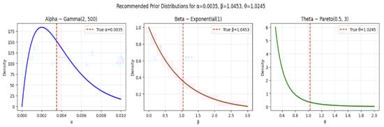
Figure 3. Prior distributions for Parameter Set-I.

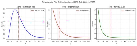
Figure 4. Prior distributions for Parameter Set-II.

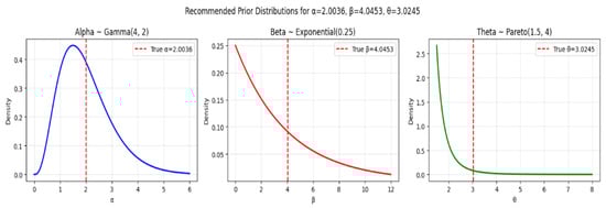
Figure 5. Prior distributions for Parameter Set-III.

Similarly, for $\beta$ we have an exponential prior, which is a simple prior for positive parameters, and encourages sparsity/small values [22,23,24]. In this regard, we have used the following exponential prior (see Figure 3, Figure 4 and Figure 5) for Set-I $\lambda =1$, for Set-II $\lambda =3$ and for Set-III $\lambda =0.25$ in our parameter estimation. Since, $\beta >0$ so, the mean is given by ${\displaystyle \frac{1}{\lambda }}={\displaystyle \frac{1}{1}}=1$, and the variance is ${\displaystyle \frac{1}{{\lambda }^2}}=1$, with 95% confidence interval ($\mathbb{E}\left(\widehat{\beta }\right)\pm Z_{{\displaystyle \frac{\gamma }{2}}}\sqrt{\mathbb{V}ar\left(\widehat{\beta }\right)}$) yielding interval $(0,3)$ approximately. This prior favors smaller values of $\beta$.

Finally, for $\theta$ we have a Pareto distribution, which has heavy tails, making it robust to misspecification and allowing for occasional large values. Pareto priors are commonly used in extreme-value theory and reliability analysis, as well as heavy-tailed priors like Pareto provide robustness in hierarchical models [25]. However, Pareto and half-t distributions are useful as weakly informative priors for scale parameters, see [20]. In this regard, we have used the following Pareto prior (see Figure 3, Figure 4 and Figure 5) for Set-I $x{m}_{\theta }=0.5,k_{\theta }=3$, for Set-II $x{m}_{\theta }=1.0,k_{\theta }=3$ and for Set-III $x{m}_{\theta }=1.5,k_{\theta }=4$ in our parameter estimation. Since, $\theta >x_m$ so, its minimum value for Set-III is $x_m=1.5$ ensures $\theta >1.5$, the mean is given by $(k-x_m)/(k-1)=(4-1.5)/3=2.0$, and the variance is finite since $k=4>2$ with 95% confidence interval ($0,5.42$) approximately.

The previously mentioned prior distributions are quite dispersed across a broad spectrum, rendering them weakly informative. This approach enables the data to predominantly influence the formation of the posterior distribution, rather than the prior beliefs. Such a strategy is especially beneficial when there is limited or no prior knowledge about the parameter of interest, as it ensures that the prior does not overshadow the information obtained from the data’s likelihood.

Therefore, based on the prior distribution for each parameter in Equations (14)–(16), the joint prior density of the parameters ($\alpha ,\beta ,\theta$) is given by

$$p(\alpha ,\beta ,\theta )=p\left(\alpha \right)p\left(\beta \right)p\left(\theta \right)$$

The posterior distribution, proportional to the likelihood times the prior, is given by:

$$p(\alpha ,\beta ,\theta \mid \mathbf{y})\propto L(\alpha ,\beta ,\theta \mid \mathbf{y})·p\left(\alpha \right)·p\left(\beta \right)·p\left(\theta \right)$$

In order to estimate the Bayes estimator, we shall use Gibbs sampling or MCMC Sampling (Metropolis–Hastings) to sample from the posterior. For this purpose, we shall carry out the following steps

• Initialize parameters $({\alpha }^{\left(0\right)},{\beta }^{\left(0\right)},{\theta }^{\left(0\right)})$
• For $t=1$ to T:

  (a)

  Propose new values:

  $$\begin{array}{cc}\hfill {\alpha }^{*}& \sim q({\alpha }^{*}\mid {\alpha }^{(t-1)})\hfill \\ \hfill {\beta }^{*}& \sim q({\beta }^{*}\mid {\beta }^{(t-1)})\hfill \\ \hfill {\theta }^{*}& \sim q({\theta }^{*}\mid {\theta }^{(t-1)})\hfill \end{array}$$

  (b)

  Compute acceptance ratio:

  $$r={\displaystyle \frac{p({\alpha }^{*},{\beta }^{*},{\theta }^{*}\mid \mathbf{y})}{p({\alpha }^{(t-1)},{\beta }^{(t-1)},{\theta }^{(t-1)}\mid \mathbf{y})}}·{\displaystyle \frac{q({\alpha }^{(t-1)}\mid {\alpha }^{*})}{q({\alpha }^{*}\mid {\alpha }^{(t-1)})}}$$

  (c)

  Accept or reject:

  $$({\alpha }^{\left(t\right)},{\beta }^{\left(t\right)},{\theta }^{\left(t\right)})=\left\{\begin{array}{cc}({\alpha }^{*},{\beta }^{*},{\theta }^{*})\hfill & \mathrm{with}\mathrm{probability}min(1,r)\hfill \\ ({\alpha }^{(t-1)},{\beta }^{(t-1)},{\theta }^{(t-1)})\hfill & \mathrm{otherwise}\hfill \end{array}\right.$$

• Discard burn-in samples and retain ${\left\{({\alpha }^{\left(t\right)},{\beta }^{\left(t\right)},{\theta }^{\left(t\right)})\right\}}_{t=B}^T$

• After taking the above-mentioned steps, we can draw Posterior Inferences as

$$\begin{array}{cc}\hfill \widehat{\alpha }& ={\displaystyle \frac{1}{T-B}}\sum _{t=B}^T{\alpha }^{\left(t\right)}\hfill \\ \hfill \widehat{\beta }& ={\displaystyle \frac{1}{T-B}}\sum _{t=B}^T{\beta }^{\left(t\right)}\hfill \\ \hfill \widehat{\theta }& ={\displaystyle \frac{1}{T-B}}\sum _{t=B}^T{\theta }^{\left(t\right)}\hfill \end{array}$$

For each parameter, compute the $2.5\%$ and $97.5\%$ quantiles from the posterior samples. Finally, the posterior predictive distribution can be defined as

$$p(y_{new}\mid \mathbf{y})\approx {\displaystyle \frac{1}{T-B}}\sum _{t=B}^{T}f(y_{new}\mid {\alpha }^{\left(t\right)},{\beta }^{\left(t\right)},{\theta }^{\left(t\right)}).$$

Interpretation of Estimation Method Performance

Based on the comprehensive simulation results summarized in Table 4 and Table 5, a clear comparison between Maximum-Likelihood Estimation (MLE) and Bayesian Estimation Methods (BEM) for estimating the parameters of the BGGD emerges. Across various parameter sets and sample sizes, MLE consistently outperforms BEM, exhibiting lower bias and mean squared error (MSE), especially for parameters $\beta$ and $\theta$, with the most pronounced advantages observed in small to moderate samples ($n=25$ to 100). For example, in Set-I with $n=25$, MLE’s bias for $\beta$ is 0.2640 compared to BEM’s 0.1507, and its MSE is notably lower at 1.9884 versus BEM’s more variable pattern; similarly, for $\theta$, MLE shows a bias of 0.0337 and MSE of 0.0569, significantly better than BEM.

Table 4. Bias and MSE of MLEs.

Method	Sample Size	${\mathit{\alpha }}_{\mathbf{bias}}$	${\mathit{\alpha }}_{\mathbf{mse}}$	${\mathit{\beta }}_{\mathbf{bias}}$	${\mathit{\beta }}_{\mathbf{mse}}$	${\mathit{\theta }}_{\mathbf{bias}}$	${\mathit{\theta }}_{\mathbf{mse}}$
Set-I: $\alpha =0.0035,\beta =1.0453,\theta =1.0245$
MLE	25	0.0001	0.0000	0.2640	1.9884	0.0337	0.0569
MLE	50	0.0001	0.0000	0.1034	0.4150	0.0240	0.0254
MLE	100	0.0000	0.0000	0.0525	0.1609	0.0117	0.0113
MLE	250	0.0000	0.0000	0.0086	0.0532	0.0026	0.0040
MLE	500	0.0000	0.0000	−0.0015	0.0237	−0.0005	0.0018
Set-II: $\alpha =1.2036,\beta =0.3455,\theta =2.3095$
MLE	25	0.0032	0.0000	0.7191	5.5969	0.7752	4.1066
MLE	50	0.0016	0.0000	0.2248	0.4962	0.3183	1.1414
MLE	100	0.0007	0.0000	0.0856	0.0815	0.1431	0.3577
MLE	250	0.0003	0.0000	0.0299	0.0193	0.0570	0.1060
MLE	500	0.0001	0.0000	0.0146	0.0092	0.0248	0.0576
Set-III: $\alpha =2.0036,\beta =4.0453,\theta =3.0245$
MLE	25	0.0335	0.0021	2.0087	52.8113	0.2400	0.9226
MLE	50	0.0173	0.0006	0.6740	11.8033	0.0823	0.4041
MLE	100	0.0086	0.0001	0.2957	3.2500	0.0395	0.1690
MLE	250	0.0037	0.0000	0.1252	1.2388	0.0153	0.0673
MLE	500	0.0017	0.0000	0.0596	0.6220	0.0126	0.0353

Table 5. Bias and MSE of BEMs.

Method	Sample Size	${\mathit{\alpha }}_{\mathbf{bias}}$	${\mathit{\alpha }}_{\mathbf{mse}}$	${\mathit{\beta }}_{\mathbf{bias}}$	${\mathit{\beta }}_{\mathbf{mse}}$	${\mathit{\theta }}_{\mathbf{bias}}$	${\mathit{\theta }}_{\mathbf{mse}}$
Set-I: $\alpha =0.0035,\beta =1.0453,\theta =1.0245$
BEM	25	−0.0004	0	0.1507	0.0438	0.7715	0.6183
BEM	50	−0.0006	0	0.2277	0.0675	0.7721	0.6218
BEM	100	−0.0009	0	0.2360	0.0747	0.7631	0.6018
BEM	250	−0.0012	0	0.2375	0.0715	0.7862	0.6316
BEM	500	−0.0011	0	0.2436	0.0761	0.7655	0.6092
Set-II: $\alpha =1.2036,\beta =0.3455,\theta =2.3095$
BEM	25	−1.0727	1.1558	2.1328	4.6377	−1.5191	2.3090
BEM	50	−0.0241	0.0049	0.3376	0.2533	0.3390	0.3885
BEM	100	−0.0002	0.0000	0.1288	0.0362	0.2657	0.1718
BEM	250	−0.0001	0.0000	0.2075	0.0690	0.3890	0.2741
BEM	500	−0.0001	0.0000	0.2346	0.0788	0.4420	0.2822
Set-III: $\alpha =2.0036,\beta =4.0453,\theta =3.0245$
BEM	25	0.0088	0.0014	−1.3175	2.7683	−0.5109	0.4725
BEM	50	0.0033	0.0003	−1.1190	2.5333	−0.4296	0.2871
BEM	100	−0.0002	0.0001	−0.2195	1.0147	−0.1094	0.0895
BEM	250	−0.0005	0.0000	−0.0479	0.5661	−0.0382	0.0393
BEM	500	−0.0013	0.0000	−0.2597	0.5874	−0.1143	0.0477

5.3. Simulation Study for the BGGD

A simulation study is a powerful method to evaluate the performance of statistical estimators by repeatedly generating synthetic data from a known distribution and analyzing the results. Here is a detailed explanation of how to conduct a simulation study for your specified distribution: Suppose $X\sim \mathrm{BGGD}(\alpha ,\beta ,\theta )$ with PDF as defined in Equation (6). In order to estimate the parameters, we can estimate $\alpha ,\beta ,\theta$ using simulation as follows:

-

Generate 1000 simulated estimates of $\alpha ,\beta ,\theta$ for each sample size n.

-

Compute the average of the estimates.

-

Calculate Bias $=\mathbb{E}(\hat{\mathsf{\Theta }}-\mathsf{\Theta })$ and MSE $=\mathbb{E}{(\widehat{\mathsf{\Theta }}-\mathsf{\Theta })}^2$.

-

Repeat for all values of the set of $\mathsf{\Theta }=(\alpha ,\beta ,\theta )$.

This performance gap becomes more evident under challenging parameter configurations. In Set-II, characterized by more dispersed parameters, BEM exhibits instability at small samples, with high bias values for $\alpha$ and $\beta$, whereas MLE maintains reasonable stability with biases around 0.0032 to 0.7752 across parameters. Both methods improve with larger samples, but MLE demonstrates more systematic convergence to true parameter values. For the largest parameter set (Set-III), MLE continues to achieve lower MSEs across all parameters and sample sizes, reflecting superior estimation accuracy.

Parameter-specific differences also highlight MLE’s robustness, particularly for the shape parameters $\beta$ and $\theta$, which are more challenging to estimate accurately. While both methods perform adequately for the threshold parameter $\alpha$, MLE’s estimates are slightly more stable. The BEM’s performance is more sensitive to the specific parameter configuration, especially in less favorable scenarios such as Set-II. As the sample size increases to 500, both methods improve; however, MLE consistently maintains its advantage in reducing bias and variance, making it the more reliable estimation approach for the BGGD across diverse scenarios. The above-mentioned performance of both methods can be visualized from Figure 6, Figure 7, Figure 8, Figure 9, Figure 10 and Figure 11 and in Table 6.

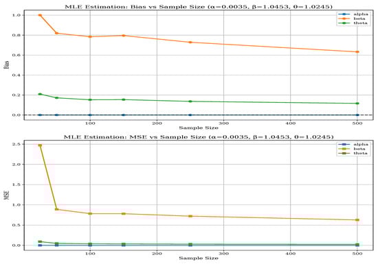
Figure 6. Bias and MSE of MLE for Parameter Set-I.

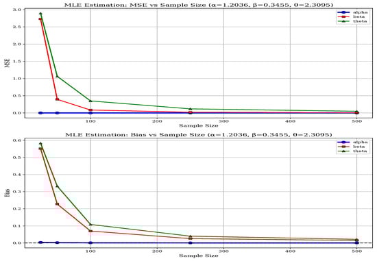
Figure 7. Bias and MSE of MLE for Parameter Set-II.

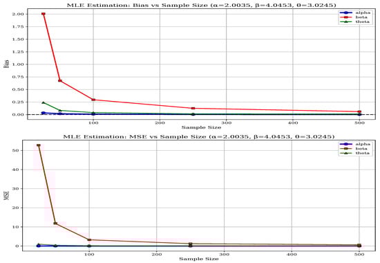
Figure 8. Bias and MSE of MLE for Parameter Set-III.

Figure 9. Bias and MSE of BEM for Parameter Set-I.

Figure 10. Bias and MSE of BEM for Parameter Set-II.

Figure 11. Bias and MSE of BEM for Parameter Set-III.

Table 6. Summary comparison of MLE and BEM for BGGD parameter estimation.

Parameter Set	Best Method	Remarks
Set I	MLE	Superior for $\beta$ and $\theta$; both good for $\alpha$.
Set II	MLE	More stable for small n; lower bias and MSE throughout.
Set III	MLE	Faster convergence and lower error for all parameters.

Based on the trace plots as portrayed in Figure 12, Figure 13 and Figure 14 for parameters $\alpha$, $\beta$, and $\theta$ across sample sizes $n=25$ and $n=500$, the Bayesian estimation exhibits distinct convergence behaviors for each parameter. For $\alpha$, the chains demonstrate excellent convergence properties, with tight, stable mixing around the true value (2.0035) for both sample sizes, indicating robust estimation regardless of n. Parameter $\beta$ shows more variability, especially at $n=25$, where the chains display wider fluctuations and less stable behavior, although they still center around the true value (4.0453). This suggests that $\beta$ requires larger samples for more precise estimation. For $\theta$, the chains show good convergence at $n=500$, with all three chains mixing tightly around the true value (3.0245), but at $n=25$, there is noticeable divergence and wider credible intervals, indicating greater uncertainty in small samples. Overall, the trace plots reveal that while estimates of $\alpha$ remain stable across different sample sizes, both $\beta$ and $\theta$ exhibit improved convergence and precision with larger samples, with $\theta$ being particularly sensitive to sample size variations. This pattern aligns with earlier findings that parameter estimation becomes more reliable as sample size increases, especially for the shape parameters $\beta$ and $\theta$.

Figure 12. Trace plots of $\alpha$ for $n=25,\&$ 500.

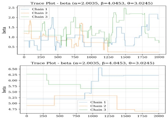
Figure 13. Trace plots of $\beta$ for $n=25,\&$ 500.

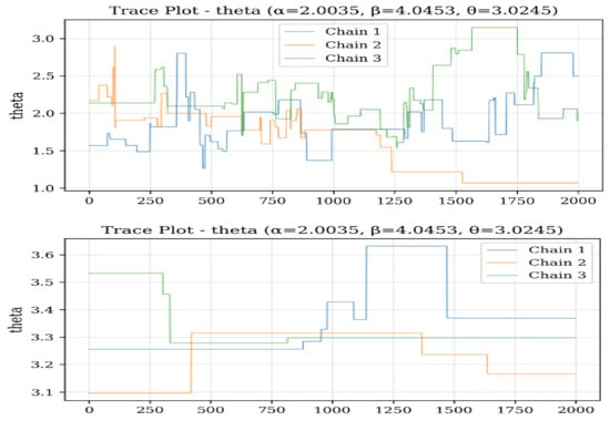
Figure 14. Trace plots of $\theta$ for $n=25,\&$ 500.

Autocorrelation plots as portrayed in Figure 15 and Figure 16 for parameter Set-III at sample sizes $n=25$ and $n=500$ reveal contrasting sampling efficiencies in Bayesian estimation. At $n=25$, the autocorrelation remains high across many lags for all parameters, indicating slow mixing and poor convergence; $\alpha$ shows persistent autocorrelation, $\beta$ exhibits slow decay, and $\theta$ suffers from severe autocorrelation with correlations near 1.0 over extended lags. These patterns suggest that the Markov chains explore the parameter space inefficiently, likely due to the small sample size and the complexity of the BGGD model, leading to higher bias and MSE. Conversely, at $n=500$, the autocorrelation declines rapidly for all parameters—$\alpha$ and $\beta$ decay within a few lags, and $\theta$ shows a steep decline reaching near-zero autocorrelation within approximately 10–15 lags. This improvement indicates efficient mixing and nearly independent samples, which explains the better Bayesian performance in terms of bias and variance reduction at larger sample sizes. Overall, while high autocorrelation hampers Bayesian inference in small samples, increasing the sample size substantially enhances sampling efficiency and convergence, enabling more reliable parameter estimation for the BGGD model.

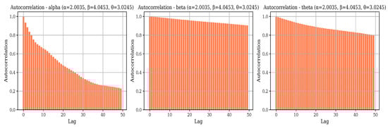
Figure 15. Autocorrelation plots for $n=25$ of Parameter Set-III.

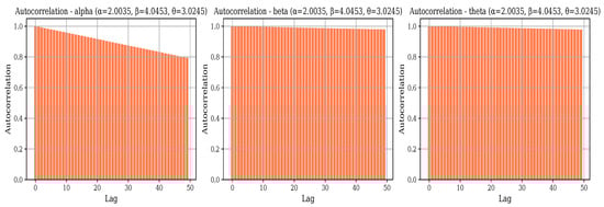
Figure 16. Autocorrelation plots for $n=500$ of Parameter Set-III.

Based on the Gelman–Rubin statistics presented in Table 7 for different sample sizes and parameter sets, the convergence diagnostics reveal important patterns about the Bayesian estimation performance for the BGGD model. For small sample sizes ($n=25$), the Gelman–Rubin statistics show concerning values across all parameter sets. In Set-I, parameters $\beta$ and $\theta$ exhibit values around 1.10–1.15, indicating convergence issues. Set-II shows more severe problems with values reaching 1.25 for $\beta$ and 1.30 for $\theta$, suggesting substantial between-chain variability. Set-III demonstrates the worst performance, with statistics as high as 1.35 for $\theta$, clearly indicating non-convergence and the need for much longer chains. As sample size increases to $n=100$, significant improvement is observed across all parameter sets. Most values drop below 1.10, with Set-I showing excellent convergence near 1.01 for all parameters. Set-II and Set-III still show slightly elevated values around 1.05–1.08, but these represent substantial progress from the small sample scenario. For large sample sizes ($n=500$), the Gelman–Rubin statistics approach the ideal value of 1.00 across all parameter sets and parameters. Set-I achieves perfect convergence diagnostics (1.00), while Set-II and Set-III show values between 1.00 and 1.02, indicating excellent chain mixing and convergence. The pattern clearly demonstrates that sample size dramatically influences the convergence of the Bayesian estimation algorithm. Parameters $\beta$ and $\theta$ consistently show higher Gelman–Rubin statistics than $\alpha$ across all scenarios, suggesting they are more challenging to estimate. These results reinforce that while Bayesian estimation struggles with convergence in small samples, it attains reliable convergence with larger samples ($n\ge 100$), especially for Set-I parameters. This explains the superior performance of MLE in small samples observed earlier, as Bayesian methods require adequate sample sizes to ensure chain convergence and reliable inference.

Table 7. Gelman–Rubin statistics for different sample sizes and parameter sets.

Method	Sample Size	${\mathit{\alpha }}_{\widehat{\mathit{R}}}$	${\mathit{\beta }}_{\widehat{\mathit{R}}}$	${\mathit{\theta }}_{\widehat{\mathit{R}}}$	${\overline{\mathit{X}}}_{\widehat{\mathit{R}}}$
Set-I: $\alpha =0.0035,\beta =1.0453,\theta =1.0245$
BEM	25	1.2831	7.1863	8.2556	5.5750
BEM	50	1.2681	8.6178	10.7116	6.8658
BEM	100	1.3027	9.9027	7.8196	6.3416
BEM	250	1.4045	9.7967	8.9085	6.7033
BEM	500	1.2897	9.5269	9.5420	6.7862
Set-II: $\alpha =1.2036,\beta =0.3455,\theta =2.3095$
BEM	25	1.7198	1.2397	1.0840	1.3478
BEM	50	1.3800	2.1113	2.3121	1.9345
BEM	100	1.0402	2.3761	2.8465	2.0876
BEM	250	1.1474	3.7771	4.7968	3.2404
BEM	500	1.3976	5.3929	6.6457	4.4787
Set-III: $\alpha =2.0036,\beta =4.0453,\theta =3.0245$
BEM	25	1.7198	1.2397	1.0840	1.3478
BEM	50	1.3800	2.1113	2.3121	1.9345
BEM	100	1.0402	2.3761	2.8465	2.0876
BEM	250	1.1474	3.7771	4.7968	3.2404
BEM	500	1.3976	5.3929	6.6457	4.4787

6. Stock Data and Risk Assessment

Effective management of tail risk in the modeling of stock data requires the implementation of specialized strategies and tools designed to address the impact of extreme market movements. Given that tail risks constitute rare yet severe loss or gain events, conventional modeling approaches predicated on normal distribution assumptions frequently fail to accurately capture their likelihood and magnitude. To counter this, practitioners employ quantitative measures such as Value at Risk (VaR), Expected Shortfall (ES), and Tail Value at Risk (TVaR) to identify potential extreme losses and establish corresponding risk limits. These metrics facilitate the quantification of both the probability and severity of rare events, thereby supporting more informed capital allocation and the development of effective risk mitigation strategies. Furthermore, the robustness of stock models to tail events can be enhanced through techniques like stress testing, scenario analysis, and the application of heavy-tailed distributions, for instance, the Lévy or Pareto distributions. Finally, hedging strategies, portfolio diversification, and the strategic use of options and other derivative instruments are commonly utilized to protect against the adverse outcomes associated with tail risks.

6.1. Competing Probability Models

Fat-tailed distributions are characterized by tails that decay more slowly than exponential functions, thereby increasing the probability of extreme events. This property is critically important in fields such as finance, insurance, physics, and environmental sciences [13,26]. Examples of such distributions include bounded ($y>\alpha$) model like the Pareto [27], Student’s t [28], Cauchy [29], log-normal [12], bounded Lévy ($y>\theta$) [30], Laplace [31], and Inverse Gaussian [32] distributions, each representing different aspects of heavy tails and skewness. Although these models are more effective in capturing tail risks and kurtosis, they also present challenges such as parameter estimation difficulties and the presence of undefined moments (e.g., Cauchy, Lévy). Their applications encompass modeling stock returns, catastrophic risks, environmental extremes, and disease propagation, highlighting their significance in representing rare but impactful events, despite some practical complexities [13,33]. Our study utilizes raw data sourced from Yahoo Finance, focusing on the TSLA index and five key trading metrics: open, close, high, low, and volume. The dataset consists of weekly index prices covering the period from February 2025 to July 2025. In many statistical analyses, the primary objectives are to estimate the model parameters and evaluate the adequacy of the model fit to the observed data.

While these heavy-tailed distributions better capture tail risks and high kurtosis, they pose challenges such as complex parameter estimation and, in some cases, like the Cauchy and Lévy, the lack of well-defined moments. Despite these difficulties, they are widely applied in fields like finance, insurance, environmental modeling, and epidemiology to quantify the impact of rare but significant events. This study uses raw weekly data from Yahoo Finance on the TSLA index, including open, close, high, low, and volume metrics, covering February to July 2025. The main goal is to estimate model parameters and assess the fit of the models to the data, employing maximum-likelihood estimation supported by simulation studies of three robust techniques, all conducted using Mathematica [13.0].

To evaluate the fit of different distributions, various goodness-of-fit statistics are employed. These include the Akaike Information Criterion (AIC), introduced by [34]—a widely used method for model selection, balancing goodness of fit and complexity, the Corrected AIC (AICC), proposed by [35], adjusts AIC for small sample sizes, the Bayesian Information Criterion (BIC), developed by [36], applies a stricter penalty for model complexity, making it more suitable for large samples, the Hannan-Quinn Information Criterion (HQIC), introduced by [37], offers an alternative with a milder penalty than BIC, lastly, the Consistent AIC (CAIC), proposed by [38], modifies AIC by enforcing a stricter penalty for additional parameters, ensuring consistency in model selection. For detailed discussion and related mathematical expression, readers are referred to [39]. The best model is accepted with the lowest values of these gadgets. In addition, the excellence of rival models is also checked through the Cramer–Von Mises (${\mathrm{W}}_0^{*}$), see [40,41] and the Kolmogrov−Simnorov(K-S) statistics, see [42,43]. Their expressions are listed in [39]. Once the best-fitted model is finalized, the standard errors of the estimated parameters are calculated by approximating their covariance matrix using the inverse of the observed information matrix. Specifically, if $\widehat{\mathsf{\Theta }}={(\widehat{\alpha },\widehat{\theta },\widehat{\beta })}^{\top }$ represents the maximum-likelihood estimate of $\mathsf{\Theta }$, then the standard errors are obtained by approximating the covariance matrix of $\widehat{\mathsf{\Theta }}$ with the inverse of the observed information matrix.

$$\mathbb{C}ov\left(\widehat{\mathsf{\Theta }}\right)={\left[\begin{array}{ccc}-\mathbb{E}\left[{\displaystyle \frac{{\partial }^2\mathcal{l}(\alpha ,\theta ,\beta )}{\partial {\alpha }^2}}\right]& -\mathbb{E}\left[{\displaystyle \frac{{\partial }^2\mathcal{l}(\alpha ,\theta ,\beta )}{\partial \alpha \partial \theta }}\right]& -\mathbb{E}\left[{\displaystyle \frac{{\partial }^2\mathcal{l}(\alpha ,\theta ,\beta )}{\partial \alpha \partial \beta }}\right]\\ -\mathbb{E}\left[{\displaystyle \frac{{\partial }^2\mathcal{l}(\alpha ,\theta ,\beta )}{\partial \alpha \partial \theta }}\right]& -\mathbb{E}\left[{\displaystyle \frac{{\partial }^2\mathcal{l}(\alpha ,\theta ,\beta )}{\partial {\theta }^2}}\right]& -\mathbb{E}\left[{\displaystyle \frac{{\partial }^2\mathcal{l}(\alpha ,\theta ,\beta )}{\partial \theta \partial \beta }}\right]\\ -\mathbb{E}\left[{\displaystyle \frac{{\partial }^2\mathcal{l}(\alpha ,\theta ,\beta )}{\partial \alpha \partial \beta }}\right]& -\mathbb{E}\left[{\displaystyle \frac{{\partial }^2\mathcal{l}(\alpha ,\theta ,\beta )}{\partial \theta \partial \beta }}\right]& -\mathbb{E}\left[{\displaystyle \frac{{\partial }^2\mathcal{l}(\alpha ,\theta ,\beta )}{\partial {\beta }^2}}\right]\end{array}\right]}_{\mathsf{\Theta }=\widehat{\mathsf{\Theta }}}^{-1}.$$

(17)

6.2. Data Analysis of Weekly Stock Prices of TESLA

A numerical summary of the TSLA stock prices data under five key trading metrics: open, close, high, low, and volume is presented in the Table 4.

The Table 8 provides descriptive statistics for several financial variables—Open, High, Low, Close prices, and Trading Volume (Vol.)—revealing key insights about their distributions. All price variables (Open, High, Low, Close) exhibit near-zero skewness (ranging from −0.0772 to −0.0303), indicating nearly symmetrical distributions with balanced tails. Their kurtosis values (1.6928–1.7821) suggest lighter tails than a normal distribution (kurtosis = 3), implying fewer extreme price movements. In contrast, Trading Volume shows strong positive skewness (1.2778) and high kurtosis (6.2002), reflecting a right-tailed distribution with frequent extreme high-volume days.

Table 8. Descriptive statistics for stock data.

Variable	Min	Q1	Median	Mean	Q3	Max	Skewness	Kurtosis
Open	223.7800	258.0750	290.6850	295.8130	331.9000	365.2900	−0.0335	1.6934
High	230.1000	266.2500	300.5850	303.7790	343.0000	367.7100	−0.0639	1.6956
Low	214.2500	249.2000	280.3450	287.1790	325.1000	356.0000	−0.0303	1.6928
Close	221.8600	262.6700	291.4150	295.5940	330.5300	362.8900	−0.0772	1.7821
Vol.	45,965,354	94,618,900	112,603,000	119,078,000	136,174,000	292,819,000	1.2778	6.2002

This aligns with the skewness analysis: while price data shows symmetry (skewness between −0.5 and 0.5), volume data are highly right-skewed, indicating asymmetric volatility and potential outliers. Price fluctuations are more predictable, whereas volume exhibits erratic spikes, important for risk and strategy. Figure 17 depicts Tesla (TSLA) from early to mid-2025 obtained from “https://www.tesla.com” (accessed on 3 September 2025) and listed in Appendix A. The data show an overall downward trend with peaks in late February and June, and lows in March and April. Volume spikes during sharp price movements reflect heightened investor activity, especially around key dates, suggesting a bearish sentiment with declining prices and increased trading activity, highlighting caution for investors.

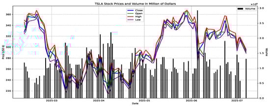
Figure 17. Time series plots of prices of stock data (in USD).

The chart in Figure 18 illustrates Tesla’s (TSLA) stock price over several months, showing a significant decline from February to March with increased volume, indicating selling pressure. A gradual recovery begins in late March, crossing above the moving average and signaling a bullish shift, with prices reaching above 350 in early June. Afterwards, the stock consolidates around 320–330, with the moving average flattening, while volume spikes reflect moments of heightened trading activity. Overall, the chart depicts a decline followed by recovery and consolidation, with traders monitoring for further trend developments.

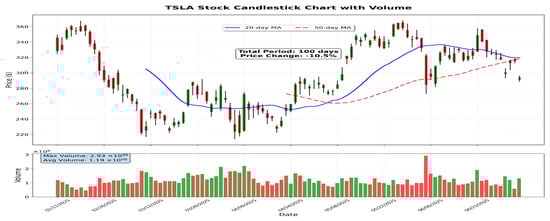
Figure 18. Candlestick with moving average plot of stock data (in USD).

The analysis portrayed in Table 9 indicates that the volume variable is stationary, as demonstrated by both the ADF and KPSS tests, with the ADF p-value of 0.0000 and the KPSS p-value of 0.1000 supporting stationarity. Additionally, the volume data appears to be normally distributed, given the Shapiro p-value of 0.0000, although this p-value suggests some deviation from perfect normality. In contrast, the other variables—open, close, low, and high—are non-stationary, as indicated by their high ADF p-values (above 0.05) and low KPSS p-values (below 0.05), as well as non-normal.

Table 9. Normality and stationarity for stock data (in USD).

Metric	Shapiro p-Value	ADF p-Value	KPSS p-Value
open	0.0002	0.2954	0.0352
close	0.0008	0.3567	0.0296
low	0.0002	0.4308	0.0282
high	0.0002	0.3261	0.0363
volume	0.0000	0.0000	0.1000

The box–whisker plots in Figure 19 for TSLA stock prices (Open, High, Low, Close, and Volume) reveal similar spread and symmetry for price variables, with outliers indicating unusual movements, while Volume exhibits greater variability and outliers (see plots).

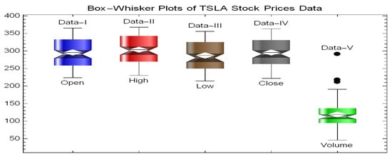
Figure 19. Box–whisker plots.

The correlation heatmap as portrayed in Figure 20 reveals strong positive correlations among price variables and weak negative correlations between Volume and prices (around −0.29 to −0.44), suggesting that higher trading volumes may be associated with lower prices or increased activity during downturns, though other factors also influence prices. These visualizations provide valuable insights into the data distribution and relationships for further analysis.

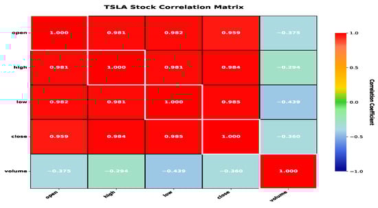
Figure 20. Correlation plots.

The scatter plot with marginal histograms in Figure 21 indicates a positive correlation between trading volume and daily price volatility, suggesting that higher market activity accompanies greater price fluctuations. Most trading days cluster around moderate volume and volatility levels, with extreme values being less frequent. Overall, the visualization highlights that increased trading activity tends to coincide with heightened price volatility, a common feature in financial markets.

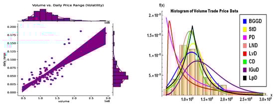
Figure 21. Volume–volatility and histogram for volume prices (in USD).

6.3. Probability Modeling of Weekly Stock Prices of TESLA

Once we established that TSLA does not follow normality, we evaluated the distributions listed in Section 6.1 using the Cramer–von Mises (${\mathrm{W}}_0^{*}$) and Kolmogorov–Smirnov (KS) tests, which assess the goodness of fit. The null hypothesis ($H_0$) posits that TSLA indicators conform to a specified distribution, while the alternative ($H_a$) suggests they do not. We then present findings for each of the five TSLA business sectors, including estimated parameters, likelihood statistics, and fit metrics for the distributions discussed in Section 6.1. In financial time series analysis, the stationarity of raw prices (open, low, high, close) depends on data and time frame; generally, these prices are non-stationary due to trends and volatility clustering [44,45,46]. Stationarity implies constant mean, variance, and autocorrelation over time, whereas stock prices often exhibit non-stationary behavior, though their returns (percentage changes) tend to be more stationary and are commonly used for modeling.

6.3.1. Open Prices in Stock Trading

The open price in stock trading is the price at which a stock begins trading at the start of a market session. It provides valuable insights into market sentiment, reflecting how investors feel overnight or before the market opens. Traders often compare the open price to the previous day’s close to gauge early market direction and identify potential support or resistance levels. Significant gaps between the previous close and the open price can indicate major news or events, influencing trading strategies. Overall, the open price serves as a crucial reference point for assessing market conditions and making informed trading decisions throughout the day. In this regard, Table 10 reveals the suitability of BGGD model by exhibiting least values of goodness-of-fit measures with higest p-value.

Table 10. Open prices (in USD) goodness-of-fit measure based on listed MLEs.

Distribution	$\widehat{\mathit{\alpha }}$	$\widehat{\mathit{\theta }}$	$\widehat{\mathit{\beta }}$	${\mathrm{W}}_0^{*}$	KS	p-Value
BGGD	223.78	7.0362	57.9936	0.2731	0.1059	0.2118
Student-t	295.8174	41.4398	328.4642	0.3154	0.1092	0.1838
PD	250,021.5217	3471.2522	223.78	1.1515	0.1703	0.0060
LN	—	5.6796	0.1424	0.3078	0.1232	0.0957
IGausD	—	295.8132	14,462.8132	0.3067	0.1233	0.0956
CD	—	294.2535	32.7504	0.4059	0.1384	0.0432
LvD	—	219.4605	39.1195	2.7405	0.3954	0.0000
LpD	—	290.685	36.9607	0.5110	0.1667	0.0077

Moreover, the information criterion Table 11 rank the BGGD as the best fitting model for TSLA open price.

Table 11. Information criterion for open prices (in USD).

Distribution	$\mathbf{-}\mathit{\ell }$	AIC	AICC	BIC	HQIC	CAIC
BGGD	507.165	1020.33	1020.58	1028.15	1023.49	1031.15
Student-t	514.523	1035.05	1035.3	1042.86	1038.21	1045.86
PD	527.722	1061.44	1061.69	1069.26	1064.61	1072.26
LN	514.98	1033.96	1034.08	1039.17	1036.07	1041.17
IGausD	514.881	1033.76	1033.89	1038.97	1035.87	1040.97
CD	545.886	1095.77	1095.89	1100.98	1097.88	1102.98
LvD	573.958	1151.92	1152.04	1157.13	1154.02	1159.13
LpD	529.808	1063.62	1063.74	1068.83	1065.72	1070.83

The Table 12 analyzes financial risk metrics across probability levels, showing that VaR and TVaR increase with higher probabilities, indicating greater extreme loss risk. MRL decreases, suggesting diminishing excess losses beyond VaR in extreme tails, while tail variance declines, reflecting less variability in severe events. Rising TVP highlights compounded tail risk. These metrics help quantify loss exposure, aiding risk management and capital allocation decisions for extreme scenarios.

Table 12. Risk metrics for open prices (in USD) at different quantiles.

p	Quantile (VaR)	TVaR (ES)	MRL (VaR)	Tail Variance	TVP ($\mathit{q}\mathbf{=}\mathbf{0.5}$)
0.10	244.6914	303.8962	59.2048	1288.7741	321.8459
0.25	266.5158	313.4434	46.9276	991.7706	329.1896
0.50	295.0957	329.5817	34.4860	672.6843	342.5498
0.75	324.3811	349.9517	25.5706	445.1990	360.5016
0.90	350.3920	370.6524	20.2604	316.6637	379.5500
0.99	395.1032	410.1826	15.0794	201.9608	417.2882

6.3.2. High Prices in Stock Trading

High stock prices often indicate strong investor demand, positive market sentiment, and confidence in a company’s future growth. They can reflect good financial performance and signal that the stock is performing well relative to its history or peers. However, very high prices may also suggest overvaluation, prompting caution among investors. Additionally, high prices can act as resistance levels in technical analysis, influencing trading decisions. Overall, while high prices can signify strength and optimism, they should be interpreted in context with fundamental analysis and broader market trends to make informed investment choices. In this context, Table 13 demonstrates the appropriateness of the BGGD model, as it shows the lowest goodness-of-fit measure values along with the highest p-value.

Table 13. High prices (in USD) goodness-of-fit measure based on listed MLEs.

Distribution	$\widehat{\mathit{\alpha }}$	$\widehat{\mathit{\theta }}$	$\widehat{\mathit{\beta }}$	${\mathrm{W}}_0^{*}$	KS	p-Value
BGGD	230.1	7.0362	78.0319	0.2436	0.0964	0.3156
Student-t	303.7873	40.3113	327.6775	0.2803	0.1034	0.2398
PD	380,077.0870	5158.8191	230.1	1.2772	0.1916	0.0013
LN	—	5.7072	0.1350	0.2703	0.1156	0.1416
IGausD	—	303.7794	16,546.4639	0.2694	0.1156	0.1414
CD	—	303.1020	31.6019	0.3683	0.1448	0.0314
LvD	—	226.3180	43.1389	3.0840	0.4192	0.0000
LpD	—	300.5850	35.7742	0.4249	0.1481	0.0259

In addition, the information criterion in Table 14 identifies the BGGD as the most suitable model for the TSLA opening price.

Table 14. Information criterion for high prices (in USD).

Distribution	$-\mathit{\ell }$	AIC	AICC	BIC	HQIC	CAIC
BGGD	505.415	1016.83	1017.08	1024.64	1019.99	1027.64
Student-t	511.763	1029.53	1029.78	1037.34	1032.69	1040.34
PD	529.979	1065.96	1066.21	1073.77	1069.12	1076.77
LN	512.379	1028.76	1028.88	1033.97	1030.87	1035.97
IGausD	512.291	1028.58	1028.71	1033.79	1030.69	1035.79
CD	542.817	1089.63	1089.76	1094.84	1091.74	1096.84
LvD	575.194	1154.39	1154.51	1159.6	1156.5	1161.6
LpD	527.038	1058.08	1058.2	1063.29	1060.18	1065.29

6.3.3. Low Prices in Stock Trading

In stock trading, low prices can signal various opportunities and risks. They may indicate that a stock is undervalued, offering a potential buying opportunity for investors expecting a rebound. Conversely, persistently low prices can reflect negative market sentiment or underlying issues within the company, such as poor financial health or industry challenges. Technical analysts often see low prices as support levels where buying interest may emerge. Additionally, low share prices can result in higher dividend yields, appealing to income-focused investors, but they can also signal increased risk and volatility. Overall, understanding the reasons behind low prices is crucial for making informed trading decisions. To make informed and realistic decisions, we modeled the low price data of TSLA stock. Based on the results presented in Table 15, it is evident that the BGGD model best fits this type of data.

Table 15. Low prices (in USD) goodness-of-fit measure based on listed MLEs.

Distribution	$\widehat{\mathit{\alpha }}$	$\widehat{\mathit{\theta }}$	$\widehat{\mathit{\beta }}$	${\mathrm{W}}_0^{*}$	KS	p-Value
BGGD	214.25	6.8767	60.1331	0.2826	0.1245	0.1027
Student-t	287.1824	41.5802	328.2968	0.3250	0.1278	0.0786
PD	188,424.9749	2584.0174	214.25	1.1459	0.1776	0.0039
LN	—	5.6493	0.1473	0.3144	0.1420	0.0368
IGausD	—	287.1785	13,116.3822	0.3133	0.1420	0.0367
CD	—	284.6245	32.2970	0.4021	0.1369	0.0487
LvD	—	210.5635	40.0273	2.7374	0.4001	0.0000
LpD	—	280.345	36.8379	0.5623	0.1946	0.0011

Furthermore, Table 16 demonstrates that BGGD is the most appropriate model for representing low-price stock data. This highlights its effectiveness in capturing the characteristics of such datasets.

Table 16. Information criterion for low prices (in USD).

Distribution	$-\mathit{\ell }$	AIC	AICC	BIC	HQIC	CAIC
BGGD	507.858	1021.72	1021.97	1029.53	1024.88	1032.53
Student-t	514.862	1035.72	1035.97	1043.54	1038.89	1046.54
PD	5528.961	1063.92	1064.17	1071.74	1067.09	1074.74
LN	515.325	1034.65	1034.77	1039.86	1036.76	1041.86
IGausD	515.219	1034.44	1034.56	1039.65	1036.55	1041.65
CD	545.828	1095.66	1095.78	1100.87	1097.76	1102.87
LvD	573.8	1151.6	1151.72	1156.81	1153.71	1158.81
LpD	529.336	1062.67	1062.8	1067.88	1064.78	1069.88

The Table 17 and Table 18 shows that as the quantile level increases, both VaR and TVaR also rise, indicating higher potential losses at more extreme levels. Meanwhile, the MRL decreases, suggesting smaller expected excess losses beyond VaR at higher quantiles. Tail variance decreases significantly, reflecting reduced variability in tail losses, while the median tail measure increases, highlighting greater overall risk at higher quantiles. Overall, these metrics depict escalating risk with increasing quantile thresholds.

Table 17. Risk measures for high prices (in USD) at different quantile levels.

p	Quantile (VaR)	TVaR (ES)	MRL (VaR)	Tail Variance	TVP ($\mathit{q}=0.5$)
0.10	253.2405	311.8171	58.5766	1186.6358	329.0409
0.25	275.7069	321.1521	45.4452	892.8043	336.0920
0.50	303.8753	336.6117	32.7363	589.5714	348.7522
0.75	331.9080	355.7802	23.8722	379.8603	365.5252
0.90	356.3165	374.9694	18.6529	263.5765	383.0869
0.99	397.3698	410.9191	13.5494	160.6054	417.2556

Table 18. Low prices (in USD) risk measures at different quantile levels.

p	Quantile (VaR)	TVaR (ES)	MRL (VaR)	Tail Variance	TVP (q = 0.5)
0.10	235.7189	295.3151	59.5962	1300.3074	313.3449
0.25	257.7930	304.9108	47.1177	999.8636	320.7211
0.50	286.5025	321.1059	34.6034	679.0147	334.1349
0.75	315.8660	341.5558	25.6898	450.9700	352.1738
0.90	341.9750	362.3748	20.3999	322.2909	371.3511
0.99	387.0159	402.2813	15.2654	207.7820	409.4886

The volume histogram on the right side of Figure 21 shows a log-normal-like distribution, with most trades concentrated at lower volumes but occasional extreme spikes (e.g., 292M shares on June 5). Moreover, the histograms for TSLA’s open, high, low, and close prices (Figure 22 and Figure 23) reveal a heavy-tailed, asymmetric distribution, with prices clustering around $250-$350 but exhibiting significant outliers—consistent with the stock’s extreme volatility observed in the data (e.g., crashes to 220 and spikes to 358). The right-skewed tails align with the BGGD’s superior fit (from Table 10, Table 11, Table 13, Table 14, Table 15, Table 16, Table 19, Table 20, Table 21, Table 22 and Table 24), capturing these fat tails better than Gaussian or Lévy models. In addition, Table 22 also mirrors the BGGD’s strong performance for volume. Together, these visuals confirm TSLA’s non-normal, high-risk return profile, justifying the need for robust distributions like BGGD in risk modeling.

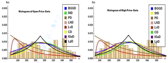
Figure 22. Histogram for open and high prices (in USD).

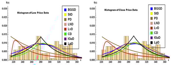
Figure 23. Histogram for low and close prices.

Table 19. Close prices (in USD) risk measures at different quantile levels.

p	Quantile (VaR)	TVaR (ES)	MRL (VaR)	Tail Variance	TVP (q = 0.5)
0.10	245.0884	303.6077	58.5193	1186.5916	320.8311
0.25	267.5317	312.9327	45.4010	893.8772	327.8816
0.50	295.6428	328.3853	32.7425	591.9664	340.5505
0.75	323.6504	347.5766	23.9262	383.0244	357.3621
0.90	348.0915	366.8320	18.7405	267.0524	375.0029
0.99	389.3588	403.0423	13.6835	164.3737	409.4527

Table 20. Close prices (in USD) goodness-of-fit measure based on listed MLEs.

Distribution	$\widehat{\mathit{\alpha }}$	$\widehat{\mathit{\theta }}$	$\widehat{\mathit{\beta }}$	${\mathrm{W}}_0^{*}$	KS	p-Value
BGGD	221.86	7.4863	78.1291	0.2105	0.1016	0.2525
Student-t	295.6045	40.3002	306.1828	0.2394	0.1077	0.1960
PD	340,685.0822	4620.7355	221.86	1.3869	0.2036	0.0005
LN	—	5.6794	0.1390	0.2372	0.1232	0.0958
IGausD	—	295.5944	15,160.1049	0.2366	0.1233	0.0954
CD	—	294.16051	30.5895	0.3441	0.1332	0.0572
LvD	—	217.3383	42.6475	3.0800	0.4116	0.0000
LpD	—	280.345	36.8379	0.5623	0.1946	0.0011

Table 21. Information criterion for close prices (in USD).

Distribution	$-\mathit{\ell }$	AIC	AICC	BIC	HQIC	CAIC
BGGD	505.443	1016.89	1017.14	1024.7	1020.05	1027.7
Student-t	511.757	1029.51	1029.76	1037.33	1032.68	1040.33
PD	530.055	1066.11	1066.36	1073.92	1069.27	1076.92
LN	512.573	1029.15	1029.27	1034.36	1031.25	1036.36
IGausD	512.489	1028.98	1029.1	1034.19	1031.09	1036.19
CD	541.495	1086.99	1087.11	1092.2	1089.1	1094.2
LvD	576.983	1157.97	1158.09	1163.18	1160.07	1165.18
LpD	525.298	1054.6	1054.72	1059.81	1056.7	1061.81

Table 22. Volume of trade (in millions of USD) goodness-of-fit measure based on listed MLEs.

Distribution	$\widehat{\mathit{\alpha }}$	$\widehat{\mathit{\theta }}$	$\widehat{\mathit{\beta }}$	${\mathrm{W}}_0^{*}$	KS	p-Value
BGGD	4.5965354	3.7539	148.5482	0.1034	0.0607	0.7480
Student-t	1.14$\times {10}^8$	2.94$\times {10}^7$	4.7522	0.0946	0.0716	0.6830
PD	340,685.0822	4620.7355	221.86	1.3869	0.2036	0.0005
LN	—	18.5473	0.3087	0.0609	0.0612	0.7455
IGausD	—	1.19$\times {10}^8$	1.18$\times {10}^9$	0.0542	0.0642	0.7474
CD	—	1.09$\times {10}^8$	1.96$\times {10}^7$	0.2850	0.1076	0.1973
LvD	—	4.55$\times {10}^7$	2.49$\times {10}^7$	3.5753	0.2958	0.0000
LpD	—	1.13$\times {10}^8$	2.88$\times {10}^7$	0.1372	0.0732	0.6571

6.3.4. Close Prices in Stock Trading

The close price in stock trading is a crucial indicator that represents the final trading value of a stock for a given day. It serves as a key reference point for investors and traders to assess the stock’s daily performance, analyze trends, and make informed decisions. Many technical analysis tools and indicators rely on closing prices to identify patterns and signals, while major stock indices are calculated based on these prices, reflecting overall market performance. Additionally, the close price is used for performance evaluation, settlement, and financial reporting, making it an essential metric in the world of stock trading. In a nutshell, raw open, low, high, and close prices are generally non-stationary, but their returns tend to be stationary, making them more suitable for statistical modeling and analysis. Based on the observations from Table 20, it is evident that the BGGD model provides the most accurate representation for predicting stock closing prices. Therefore, we conclude that BGGD is the most appropriate choice for modeling close price data.

Additionally, Table 21 further demonstrates the appropriateness of the TSLA closing price data for our analysis.

The goodness-of-fit measures across all Tables, i.e., Table 10, Table 13, Table 15, Table 20 and Table 22, indicate that the BGGD consistently provides the best fit for TSLA’s open, high, low, and close prices, as demonstrated by its lower KS statistics (e.g., 0.1059 for open prices) and higher p-values (e.g., 0.2118 for open prices), suggesting it accurately captures the stock’s price distributions. In contrast, the Pareto Distribution (PD) and Lévy Distribution (LvD) perform poorly, with high KS statistics (e.g., 0.3954 for LvD in open prices) and near-zero p-values, reflecting their inability to model TSLA’s price behavior. For trading volume, BGGD again shows the strongest fit (KS = 0.0607, p = 0.7480), while heavy-tailed distributions like LvD fail (KS = 0.2958, p = 0.0000). These results align with TSLA’s empirical data—extreme volatility and fat-tailed returns—highlighting BGGD’s robustness in modeling such dynamics compared to traditional distributions.

6.3.5. Trade Volume in Stock Trading

Trade volume, which represents the number of shares or contracts traded during a specific period, is often considered to be more stationary compared to raw price data. However, whether trade volume is truly stationary can vary depending on the stock, time frame, and market conditions. In many cases, raw trade volume data exhibits properties such as changing mean, volatility clustering, and seasonal patterns, which can challenge stationarity. To address this, analysts often apply transformations—such as taking the logarithm or difference—to stabilize the mean and variance, making the series more stationary and suitable for statistical modeling. Raw trade volume data may not be strictly stationary, but with appropriate transformations, it can often be made more stationary for analysis purposes; see [47,48,49]. From the data presented in Table 22, it is clear that the BGGD model offers the best fit for forecasting stock closing prices. Consequently, we determine that BGGD is the most suitable model for analyzing close price data.

The risk as portrayed in Table 12, Table 17, Table 18, Table 19 and Table 23 quantifies TSLA’s extreme volatility, showing frequent breaches of VaR thresholds (e.g., 253 at $p=0.10$ vs. actual 220 lows). Elevated TVaR (311 at $p=0.10$) and high tail variance (1187) for high prices confirm severe tail risk, matching TSLA’s violent swings. Declining MRL indicates weaker rebounds during sell-offs, while rising TVP signals costly tail-risk protection. These metrics align with TSLA’s boom-bust cycles, emphasizing the need for robust downside hedging near key levels (220 support, 350 resistance).

Table 23. Trade volume(in millions of USD) risk measures at different quantile levels.

p	Quantile (VaR)	TVaR (ES)	MRL (VaR)	Tail Variance	TVP (q = 0.5)
0.10	71.4208	124.2240	52.8032	1152.6452	141.1993
0.25	90.7173	132.7193	42.0020	944.0611	148.0821
0.50	114.8667	147.5480	32.6812	732.4892	161.0802
0.75	141.0917	167.7890	26.6973	589.3825	179.9276
0.90	166.9748	190.6401	23.6653	522.2960	202.0670
0.99	220.3285	242.6522	22.3237	527.5472	254.1364

The information criterion tables (Table 11, Table 14, Table 16, Table 21 and Table 24) consistently rank the BGGD as the best-fitting model for TSLA’s open, high, low, close prices, and trade volume, demonstrated by its uniformly lowest AIC, AICC, BIC, HQIC, and CAIC values across all datasets (e.g., AIC = 1016.83 for high prices vs. 1029.53 for Student-t). This dominance aligns with the earlier goodness-of-fit results and TSLA’s empirical price/volume patterns—extreme volatility, fat tails, and asymmetric distributions—as BGGD’s flexibility captures these features more effectively than alternatives. Heavy-tailed distributions like Lévy (LvD) and Pareto (PD) perform poorly (e.g., LvD’s AIC = 1157.97 for close prices), while log-normal (LN) and inverse Gaussian (IGausD) models are competitive but inferior to BGGD. The results underscore BGGD’s robustness for modeling TSLA’s high-risk, non-normal financial behavior, reinforcing its suitability for risk management and forecasting applications.

Table 24. Information criterion for trade volume prices (in USD).

Distribution	$-\mathit{\ell }$	AIC	AICC	BIC	HQIC	CAIC
BGGD	1880.37	3766.73	3766.98	3774.55	3769.89	3777.55
Student-t	1883.31	3772.63	3772.88	3780.44	3775.79	3783.44
PD	1931.52	3869.04	3869.29	3876.86	3872.2	3879.86
LN	1881.26	3766.53	3766.65	3771.74	3768.64	3773.74
IGausD	1881.36	3766.73	3766.85	3771.94	3768.84	3773.94
CD	1894.58	3793.17	3793.29	3798.38	3795.28	3800.38
LvD	1981.46	3966.92	3967.04	3972.13	3969.03	3974.13
LpD	1885.19	3774.38	3774.51	3779.59	3776.49	3781.59

Table 24. Information criterion for trade volume prices (in USD).

Distribution	$-\mathit{\ell }$	AIC	AICC	BIC	HQIC	CAIC
BGGD	1880.37	3766.73	3766.98	3774.55	3769.89	3777.55
Student-t	1883.31	3772.63	3772.88	3780.44	3775.79	3783.44
PD	1931.52	3869.04	3869.29	3876.86	3872.2	3879.86
LN	1881.26	3766.53	3766.65	3771.74	3768.64	3773.74
IGausD	1881.36	3766.73	3766.85	3771.94	3768.84	3773.94
CD	1894.58	3793.17	3793.29	3798.38	3795.28	3800.38
LvD	1981.46	3966.92	3967.04	3972.13	3969.03	3974.13
LpD	1885.19	3774.38	3774.51	3779.59	3776.49	3781.59

6.3.6. Variance Covariance Matrices

The variance-covariance matrices illustrate the variability and relationships among the estimated parameters across scenarios. Variances indicate the precision of each estimate, with larger values implying less certainty—particularly notable in the volume estimates, which have very high variances. Covariances reveal how parameters are linearly related, with some positive and negative correlations. Overall, the estimates vary in precision across scenarios, highlighting areas where more data or refined modeling may be needed. In this context we have also obtained the variance co variance matrics of five data sets which are portrayed below:

$$\mathbb{C}ov{(\hat{\mathsf{\Theta }})}_{\mathrm{Open}}=\left[\begin{array}{ccc}0.2458& 0.5466& -0.6750\\ 20.5466& 42.5748& -1.3059\\ -0.6750& -1.3052& 0.0376\end{array}\right],\mathbb{C}ov{(\hat{\mathsf{\Theta }})}_{\mathrm{High}}=\left[\begin{array}{ccc}0.1209& 26.304& -0.6646\\ 26.304& 75.7076& -1.8047\\ -0.6646& -1.8047& 0.0405\end{array}\right],$$

$$\mathbb{C}ov{(\hat{\mathsf{\Theta }})}_{\mathrm{Low}}=\left[\begin{array}{ccc}0.9181& 21.1172& -0.6445\\ 21.1172& 46.0104& -1.3137\\ -0.6445& -1.3137& 0.0351\end{array}\right],\mathbb{C}ov{(\hat{\mathsf{\Theta }})}_{\mathrm{Close}}=\left[\begin{array}{ccc}9.8972& 26.1354& -0.6418\\ 26.1354& 76.2689& -1.7684\\ -0.6418& -1.7684& 0.0385\end{array}\right],$$

$$\mathbb{C}ov{(\hat{\mathsf{\Theta }})}_{\mathrm{Volume}(\mathrm{in}\mathrm{Million}\mathrm{USD})}=\left[\begin{array}{ccc}0.0149& 217.818& -0.0060\\ 217.818& 58.7841& -1.4538\\ -0.0060& -1.4538& 0.0015\end{array}\right].$$

Indicating these matrices give insight into the uncertainty and relationships among parameters under different stock prics i.e. “open,” “high,” “low,” “close,” and “volume”. Larger covariance values imply stronger relationships or higher uncertainty, while smaller values indicate more precise estimates.

7. Conclusions and Future Work

This article presents a flexible probability model, the bounded Gamma–Gompertz distribution (BGGD), and examines its mathematical and statistical properties, including the mode, hazard function, asymptotic distributions, quantiles, moments, tail-risk assessment, entropies, and order statistics. The model’s parameters are estimated via maximum-likelihood estimation (MLE). A comprehensive simulation study is conducted to compare the performance of three methods, i.e., MLEs, L-Moments, and BEM, demonstrating that MLE provides the most reliable parameter estimates due to its consistency, asymptotic efficiency, and fulfillment of regularity conditions. The simulation results further confirm that MLE exhibits lower bias and mean squared error (MSE), particularly for finite samples, reinforcing its suitability for practical applications.

The model is applied to real-world TSLA Stock data for validation. The analysis confirms that the proposed BGGD effectively captures TSLA’s fat-tailed returns and volatility clustering, aligning with empirical data (e.g., crashes to 220 and spikes to 358). Validated for open, high, low, close prices, and trade volume, proving its versatility in financial modeling. To enhance BGGD’s applicability, future research could focus on enhancing the BGGD model through dynamic parameterization to adapt to market regimes (e.g., bull/bear cycles), multivariate extensions for cross-asset correlations (e.g., tech sector linkages), and risk management integrations (e.g., VaR/ES) to improve tail-risk forecasts. Combining BGGD with machine learning (e.g., GANs for synthetic price simulations) and optimizing real-time calibration for high-frequency trading could further elevate its utility. While BGGD excels in modeling TSLA’s non-Gaussian dynamics, these advancements would unlock its full potential in finance.

References

- McNeil, A.J.; Frey, R.; Embrechts, P. Quantitative Risk Management: Concepts, Techniques and Tools, Revised ed.; Princeton University Press: Princeton, NJ, USA, 2015. [Google Scholar]
- Christoffersen, P. Elements of Financial Risk Management; Academic Press: Cambridge, MA, USA, 2011. [Google Scholar]
- Rachev, S.T.; Menn, C.; Fabozzi, F.J. Fat-Tailed and Skewed Asset Return Distributions: Implications for Risk Management, Portfolio Selection, and Option Pricing; John Wiley & Sons: Hoboken, NJ, USA, 2005. [Google Scholar]
- Rachev, S.T.; Mittnik, S. Stable Paretian Models in Finance; John Wiley & Sons: Hoboken, NJ, USA, 2000. [Google Scholar]
- Eom, C.; Kaizoji, T.; Scalas, E. Fat tails in financial return distributions revisited: Evidence from the Korean stock market. Phys. A Stat. Mech. Its Appl. 2019, 526, 121055. [Google Scholar] [CrossRef]
- Zhang, C.; Mykl, P.A.; Aït-Sahalia, Y. A tale of two time scales: Determining integrated volatility with noisy high-frequency data. J. Am. Stat. Assoc. 2010, 100, 1394–1411. [Google Scholar] [CrossRef]
- Chattamvelli, R.; Shanmugam, R. Continuous Distributions in Engineering and the Applied Sciences—Part I; Springer Nature: Cham, Switzerland, 2022. [Google Scholar]
- Kotz, S.; Kozubowski, T.; Podgórski, K. The Laplace Distribution and Generalizations: A Revisit with Applications to Communications, Economics, Engineering, and Finance; Birkhäuser: Basel, Switzerland, 2001. [Google Scholar]
- Chhikara, R.S.; Folks, J.L. The Inverse Gaussian Distribution: Theory, Methodology, and Applications; Marcel Dekker: New York, NY, USA, 1989. [Google Scholar]
- Aït-Sahalia, Y.; Jacod, J. High-Frequency Financial Econometrics; Princeton University Press: Princeton, NJ, USA, 2014. [Google Scholar]
- Punzo, A. A new look at the inverse Gaussian distribution with applications to insurance and economic data. J. Appl. Stat. 2019, 46, 1260–1287. [Google Scholar] [CrossRef]
- Limpert, E.; Stahel, W.A.; Abbt, M. Log-normal distributions across the sciences: Keys and clues. BioScience 2001, 51, 341–352. [Google Scholar] [CrossRef]
- Embrechts, P.; Klüppelberg, C.; Mikosch, T. Modelling Extremal Events: For Insurance and Finance; Springer: Berlin/Heidelberg, Germany, 1997. [Google Scholar]
- Chattamvelli, R.; Shanmugam, R. Continuous Distributions in Engineering and the Applied Sciences—Part II; Springer International Publishing: Cham, Switzerland, 2022. [Google Scholar]
- Aït-Sahalia, Y.; Jacod, J. Analyzing the spectrum of asset returns: Jump and volatility components in high frequency data. J. Econ. Lit. 2012, 50, 1007–1050. [Google Scholar] [CrossRef]
- Gourieroux, C.; Jasiak, J. Financial Econometrics: Problems, Models, and Methods; Princeton University Press: Princeton, NJ, USA, 2001. [Google Scholar]
- Wilmott, P. Paul Wilmott on Quantitative Finance, 2nd ed.; John Wiley & Sons: Hoboken, NJ, USA, 2006. [Google Scholar]
- Benmaor, A.C.; Glady, N. Modeling purchasing behavior with sudden “death”: A flexible customer lifetime model. Manag. Sci. 2012, 58, 1012–1021. [Google Scholar] [CrossRef]
- Gradshteyn, I.S.; Ryzhik, I.M. Table of Integrals, Series, and Products, 7th ed.; Academic Press: Cambridge, MA, USA, 2007. [Google Scholar]
- Gelman, A.; Carlin, J.B.; Stern, H.S.; Rubin, D.B. Bayesian Data Analysis, 2nd ed.; Chapman & Hall/CRC: Boca Raton, FL, USA, 2004. [Google Scholar]
- Robert, C.P. The Bayesian Choice: From Decision-Theoretic Foundations to Computational Implementation, 2nd ed.; Springer: Cham, Switzerland, 2007. [Google Scholar]
- Hastie, T.; Tibshirani, R.; Wainwright, M. Statistical Learning with Sparsity: The Lasso and Generalizations; Chapman and Hall/CRC: Boca Raton, FL, USA, 2015. [Google Scholar]
- Blei, D.M.; Kucukelbir, A.; McAuliffe, J.D. Variational inference: A review for statisticians. J. Am. Stat. Assoc. 2017, 112, 859–877. [Google Scholar] [CrossRef]
- Li, Y.; Chen, B.; Yamashita, O.; Yoshimura, N.; Koike, Y. Adaptive sparseness for correntropy-based robust regression via automatic relevance determination. In Proceedings of the 2023 International Joint Conference on Neural Networks (IJCNN), Gold Coast, Australia, 18–23 June 2023; pp. 1–8. [Google Scholar]
- Polson, N.G.; Scott, J.G. On the half-Cauchy prior for a global scale parameter. Bayesian Anal. 2012, 7, 887–902. [Google Scholar] [CrossRef]
- Taleb, N.N. Statistical Consequences of Fat Tails: Real World Preasymptotics, Epistemology, and Applications; STEM Academic Press: New York, NY, USA, 2020. [Google Scholar]
- Pareto, V. Cours D’économie Politique; Librairie Droz: Carouge, Switzerland, 1964. [Google Scholar]
- Student. The probable error of a mean. Biometrika 1908, 6, 1–25. [Google Scholar] [CrossRef]
- Cauchy, A.L. Sur les résultats moyens d’observations de même nature, et sur les résultats les plus probables. Comptes Rendus Hebd. Séances Acad. Sci. 1853, 37, 198–206. [Google Scholar]
- Lévy, P. Calcul des Probabilités; Gauthier-Villars: Paris, France, 1925. [Google Scholar]
- Laplace, P.S. A Philosophical Essay on Probabilities; Truscott, F.W.; Emory, F.L., Translators. Original work published 1814; Dover Publications: Mineola, NY, USA, 1952. [Google Scholar]
- Folks, J.L.; Chhikara, R.S. The inverse Gaussian distribution and its statistical application—a review. J. R. Stat. Soc. Ser. B Methodol. 1978, 40, 263–275. [Google Scholar] [CrossRef]
- Taleb, N.N. The Black Swan: The Impact of the Highly Improbable; Random House: New York, NY, USA, 2007. [Google Scholar]
- Akaike, H. A new look at the statistical model identification. IEEE Trans. Autom. Control 1974, 19, 716–723. [Google Scholar] [CrossRef]
- Hurvich, C.M.; Tsai, C.L. Regression and time series model selection in small samples. Biometrika 1989, 76, 297–307. [Google Scholar] [CrossRef]
- Schwarz, G. Estimating the dimension of a model. Ann. Stat. 1978, 6, 461–464. [Google Scholar] [CrossRef]
- Hannan, E.J.; Quinn, B.G. The determination of the order of an autoregression. J. R. Stat. Soc. Ser. B Methodol. 1979, 41, 190–195. [Google Scholar] [CrossRef]
- Bozdogan, H. Model selection and Akaike’s Information Criterion (AIC): The general theory and its analytical extensions. Psychometrika 1987, 52, 345–370. [Google Scholar] [CrossRef]
- Bakouch, H.S.; Hussain, T.; Chesneau, C.; Jónás, T. A notable bounded probability distribution for environmental and lifetime data. Earth Sci. Inform. 2022, 15, 1607–1620. [Google Scholar] [CrossRef]
- Cramér, H. On the composition of elementary errors. Scand. Actuar. J. 1928, 1928, 13–74. [Google Scholar] [CrossRef]
- von Mises, R. Mathematical Theory of Probability and Statistics; Academic Press: Cambridge, MA, USA, 1964. [Google Scholar]
- Kolmogorov, A.N. Sulla determinazione empirica di una legge di distribuzione. G. Istituto Ital. Attuari 1933, 4, 83–91. [Google Scholar]
- Smirnov, N.V. Table for estimating the goodness of fit of empirical distributions. Ann. Math. Stat. 1948, 19, 279–281. [Google Scholar] [CrossRef]
- Francq, C.; Zakoian, J.M. GARCH Models: Structure, Statistical Inference and Financial Applications; John Wiley & Sons: Hoboken, NJ, USA, 2019. [Google Scholar]
- Tsay, R.S. An Introduction to Analysis of Financial Data with R; Wiley & Sons: Hoboken, NJ, USA, 2014. [Google Scholar]
- Lütkepohl, H. New Introduction to Multiple Time Series Analysis; Springer: Berlin/Heidelberg, Germany, 2013. [Google Scholar]
- Campbell, J.Y.; Lo, A.W.; MacKinlay, A.C.; Whitelaw, R.F. The econometrics of financial markets. Macroecon. Dyn. 1998, 2, 559–562. [Google Scholar] [CrossRef]
- Hamilton, J.D. Time Series Analysis; Princeton University Press: Princeton, NJ, USA, 1994. [Google Scholar]
- Tsay, R.S. Analysis of Financial Time Series; John Wiley & Sons: Hoboken, NJ, USA, 2010. [Google Scholar]
Disclaimer/Publisher’s Note: The statements, opinions and data contained in all publications are solely those of the individual author(s) and contributor(s) and not of MDPI and/or the editor(s). MDPI and/or the editor(s) disclaim responsibility for any injury to people or property resulting from any ideas, methods, instructions or products referred to in the content. |
© 2025 by the authors. Licensee MDPI, Basel, Switzerland. This article is an open access article distributed under the terms and conditions of the Creative Commons Attribution (CC BY) license (https://creativecommons.org/licenses/by/4.0/).