Numerical Investigation on Wave-Induced Boundary Layer Flow over a Near-Wall Pipeline

Abstract

Pipelines and power cables are critical infrastructures in coastal areas for transporting energy resources from offshore renewable installations to onshore grids. It is important to investigate the hydrodynamic forces on pipelines and cables and their surrounding flow fields, which are highly related to their on-bottom stability. The time-varying hydrodynamic forces coefficients and unsteady surrounding flows of a near-seabed pipeline subjected to a wave-induced oscillatory boundary layer flow are studied through numerical simulations. The Keulegan–Carpenter numbers of the oscillatory flow are up to 400, which are defined based on the maximum undisturbed near-bed orbital velocity, the pipeline diameter and the period of the oscillatory flow. The investigated Reynolds number is set to $1\times {10}^4$, defined based on $U_w$ and $D$. The influences of different seabed roughness ratios $k_s/D$ (where $k_s$ is the Nikuradse equivalent sand roughness) up to 0.1 on the hydrodynamic forces and the flow fields are considered. Both a wall-mounted pipeline with no gap ratio to the bottom wall and a pipeline with different gap ratios to the wall are investigated. The correlations between the hydrodynamic forces and the surrounding flow patterns at different time steps during one wave cylinder are analyzed by using the force partitioning method and are discussed in detail. It is found that there are influences of the increasing $k_s/D$ on the force coefficients at large $\mathrm{K}\mathrm{C},$ while for the small $\mathrm{K}\mathrm{C}$, the inertial effect from the oscillatory flow dominates the force coefficients with small influences from different $k_s/D$. The FPM analysis shows that the elongated shear layers from the top of the cylinder contribute to the peak values of the drag force coefficients.

1. Introduction

Subsea power cables serve as increasingly important infrastructures with the development of offshore renewable energy. These power cables, used to transmit electric power, are inevitably placed close to the seabed. The seabed is characterized by different roughness conditions. According to [1,2,3], the typical outer diameter of the cables is usually smaller than 200 mm, which is much smaller than that of pipelines in the oil and gas industry (usually ranging from 0.05 to 0.1 m [4]). As a result, these cables are fully immersed within the boundary layer flows near the seabed. Therefore, the influences of the boundary layer flow on the hydrodynamics of the cables as well as their on-bottom stability become significant. Furthermore, due to the vast deployment of offshore wind farms in areas with strong winds to harness high wind energy, power cables are subjected to strong wave-induced oscillatory flows, which are often characterized by high Keulegan–Carpenter ($\mathrm{K}\mathrm{C}$) numbers, defined as $\mathrm{K}\mathrm{C}=U_w{T}_w/D$ (where $U_w$ is the near-seabed orbital velocity amplitude of the oscillatory flow and $T_w$ is the wave period and $D$ is the diameter of the power cable) ([5,6,7,8]). Based on [1], strong wave conditions will lead to a large value of $U_w$ and due to the small diameter of the cables, the value of $\mathrm{K}\mathrm{C}$ can reach to orders of O(10³). The orbital motions of the water particles induced by the wave become flattened and lead to oscillatory boundary layer flows in the vicinity of the seabed. Also, due to the large seabed roughness to the cable diameter $D$ ratio $k_s/D$ ($k_s$ is defined as the Nikuradse’s equivalent roughness of the seabed), the larger boundary layer thickness and a higher turbulence intensity can be generated around the near-seabed cables, which significantly influences the hydrodynamic characteristics of the cables. According to [1], the value of $k_s/D$ can be up to O(10) when they are laid on a rocky seabed.

Due to the importance of the hydrodynamic characteristics of the cables to their on-bottom stability, many experimental and numerical studies have been performed to investigate their dependence on various parameters such as $\mathrm{K}\mathrm{C}$, $k_s/D$ and also the gap ratio between the cable and the seabed $G/D$ ($G$ is the distance of the center of the cable to the seabed). Different surrounding flow patterns can be observed under different parameters, which then leads to varying hydrodynamic force coefficients, as investigated in [9,10,11]. Early experiments conducted by [12] on the hydrodynamic force coefficients of a near-bottom-wall cylinder revealed the effects of the oscillatory boundary layer flows at $0<\mathrm{K}\mathrm{C}<60$. Two-dimensional (2D) numerical simulations were carried out by [13] at gap ratios of $G/D=0~3$. Steady streaming flow patterns around a cylinder were observed. Other 2D numerical studies such as [14,15,16] focused on the scour process beneath the pipelines at low $\mathrm{K}\mathrm{C}$ numbers. Sun et al. [17] investigated the oscillatory flow around a near-wall rectangular cylinder at different $\mathrm{K}\mathrm{C}$ in the range of $1<\mathrm{K}\mathrm{C}<20$ and $G/D$s using numerical simulations. The asymmetric pressure distributions on the cylinder due to the vicinity of the bottom wall and their correlation with vortex shedding were explored. With the increasing $\mathrm{K}\mathrm{C}$ and $k_s/D$, there is significant velocity reduction within the boundary layer flow. According to [1,18,19], ignoring the velocity reduction at high $\mathrm{K}\mathrm{C}$ will lead to an overly conservative on-bottom stability design of small-diameter cables. Most of the numerical simulation studies such as [11,13,14,17] focused on low $\mathrm{K}\mathrm{C}$ flows at $\mathrm{K}\mathrm{C}<100$. Despite that, the experimental studies of [1] were based on various oscillatory boundary layer flow conditions and the dependence of hydrodynamic coefficients on flow parameters were revealed, only statistical results of the hydrodynamic forces are reported. There is limited discussion on the influences of the oscillatory boundary layers on the surrounding flow patterns, especially at high KC, and their correlations with the hydrodynamic coefficients. For numerical simulations, the implementation of oscillatory boundary layer conditions is usually challenging. In [19], a sufficiently long domain with a length of 700D is employed to allow for the fully developed boundary layer flows. In [20], a series of preliminary 1D simulations under different flow parameters are required to be performed to obtain time-dependent and vertical varying velocity profiles at different time steps, which are implemented at the inlet. These additional simulations will increase the computational cost to the parametric study for investigating different flow characteristics of the near-wall cylinder.

In the present study, the hydrodynamic characteristics and the surrounding flow patterns of a cylinder near a rough seabed subjected to a wave-induced oscillatory boundary layer flow are investigated through numerical simulations. The influences of high $\mathrm{K}\mathrm{C}$ up to 400 and different $G/D$ and $k_s/D$ are considered. By carrying out numerical simulations under various flow conditions, detailed spatial–temporal information of the flow fields, including the coherent flow structures, can be obtained. The correlations of the surrounding flow patterns with the hydrodynamic forces on the cylinder are explored.

2. Numerical Setup

2.1. Governing Equations

Two-dimensional numerical simulations are performed to investigate the hydrodynamic coefficients of the near-wall cylinder and the surrounding flow fields. The two-dimensional Reynolds-averaged Navier–Stokes equations for the conservation of mass and momentum of the flow are solved given as

$${\displaystyle \frac{\partial u_i}{\partial x_i}}=0$$

(1)

$${\displaystyle \frac{\partial u_i}{\partial t}}+u_j{\displaystyle \frac{\partial u_i}{\partial x_j}}=-{\displaystyle \frac{1}{\rho }}\left({\displaystyle \frac{\partial P}{\partial x_i}}\right)+\nu {\displaystyle \frac{{\partial }^2{u}_i}{\partial {x_j}^2}}-{\displaystyle \frac{\partial \overline{{u_i}^{\prime }{u_j}^{\prime }}}{\partial x_j}}$$

(2)

where $i,j=1, 2$ (for $x,y$) represent the streamwise and cross-stream directions, respectively; $u_1$ and $u_2$ (for $u$ and $v$) refer to the corresponding Reynolds-averaged velocity components. $\overline{{u_i}^{\prime }{u_j}^{\prime }}$ is the Reynold stress component and ${u_i}^{\prime }$ represents the fluctuations of the velocities. $P$ is the Reynolds-averaged pressure and $\rho$ is the fluid density. The Reynolds stress tensor based on the Boussinesq eddy viscosity assumption is given by

$$\overline{{u_i}^{\prime }{u_j}^{\prime }}={\tau }_{ij}={\nu }_t\left({\displaystyle \frac{\partial u_i}{\partial x_j}}+{\displaystyle \frac{\partial u_j}{\partial x_i}}\right)-{\displaystyle \frac{2}{3}}k{\delta }_{ij}$$

(3)

where ${\nu }_t$ denotes the turbulent eddy viscosity required to be resolved by the turbulence model, $k$ is the turbulent kinetic energy and ${\delta }_{ij}$ is the Kronecker function. To resolve the turbulent eddy viscosity, the $k-\omega$ Shear Stress Transport (SST) turbulent model is employed in the present study. Detailed information on the $k-\omega$ SST turbulence model can be found in [21] and has also been used for the boundary layer flows over a near-wall cylinder in [17,19,20]. OpenFOAM, an open-source computational fluid dynamic (CFD) code based on the finite volume method (FVM) is employed to solve the governing equations. The spatial discretization schemes for the gradient, Laplacian and divergence terms and the temporal discretization for the time derivative term in the governing equations are the same as those in [20]. The solver pimpleFoam, based on the pressure implicit with pressure implicit with splitting of operators algorithms, is employed for the time integration of the unsteady flow.

2.2. Computational Overview

The computational domain is a 2D rectangular box, shown in Figure 1, with a size of $L_x\times L_z=40D\times 20D$, where $D$ is the diameter of the cylinder, as a simplified model for the near-wall power cable. The origin of the coordinates is located at the center of the cylinder. The length of the computational domain is the same as those used in [15,22] but much smaller than those used in [23] ($L_x=500D$) and [19] ($L_x=700D$). Both a wall-mounted cylinder with no gap ratio to the wall and a cylinder with gap ratios $G/D$ are considered. For the wall-mounted cylinder case, there is a small embedment of $e/D=0.05$ for the convenience of meshing.

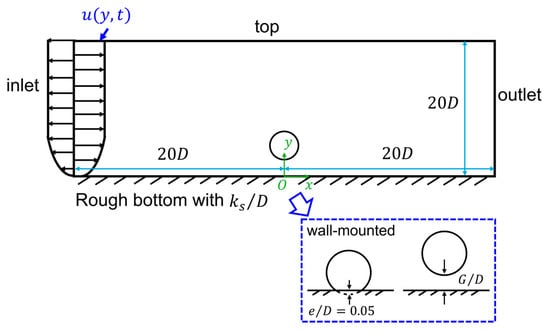
Figure 1. The computational domain. Both the wall-mounted case and a near-wall cylinder with a gap ratio are considered.

• At the inlet, fully developed time-dependent oscillatory boundary layer flow profiles are prescribed. A series of 1D numerical simulations driven by the 1D body force of the waves is performed to obtain the velocity profiles under different variables of the flow (i.e., $U_w$, $T_w$ and $k_s$). The 1D body force is given based on [15] as $F_x=U_w\mathsf{\Omega }\mathrm{c}\mathrm{o}\mathrm{s}\left(2\pi t/T_w\right)$. In addition, at the inlet, the turbulence quantities are set as zero normal gradients, as used in [19].
• At the outlet, the pressure is set as a fixed value of zero. The velocity components and the turbulence quantities are prescribed as zero normal gradient boundary conditions. These boundary conditions are the same as used in [24,25,26].
• A symmetry boundary condition is applied at the top boundary. The vertical velocity $u_y$ is zero and the horizontal velocity $u_x$ and other quantities of the simulations are set as zero normal gradient.
• At the surface of the cylinder, a no-slip condition is used for the velocity components. For the turbulence quantities, a wall function based on Spalding’s law of the wall (Spalding, [27]) is employed for the near-wall region around the cylinder surface.
• On the rough bottom wall, a no-slip condition is used for the velocity components. A zero normal gradient is used for the turbulence kinetic energy $k$. To model the roughness, the value of $\omega$ is prescribed based on Wilcox [28] as $\omega =S_r{u}_{\ast }^{+}/\nu$, where the value of $S_r$ is given as

$$S_r=\left\{\begin{array}{c}{(50/k_s^{+})}^2,k_s^{+}<25 \\ 100/k_s^{+},k_s^{+}>25\end{array}\right.$$

(4)

In this equation, the dimensionless roughness $k_s^{+}$ is given as $k_s^{+}=\left(k_s{u}_{\ast }\right)/\nu$ and $u_{\ast }$ is the friction velocity at the wall. This boundary condition is also used in [19,20,29] to model the roughness.

The force partitioning method (FPM) proposed by [30] aims to decompose the hydrodynamic forces acting on a body immersed inside a fluid into different components. This method can quantify the contribution of the surrounding flows of the immersed structure to the hydrodynamic forces without integrating the pressure on the structure, which provides a good physical insight into the correlations between the hydrodynamic forces and the coherent flow structures, especially vortices. This analysis has been employed by [31,32,33,34,35,36]. For a stationary structure such as the cylinder in the present study, the total hydrodynamic force components $F_i$ ($i=x,y$ represent the streamwise and cross-stream directions) can be decomposed as

$$F_i=-\int \left(\mathbf{u}\times \mathsf{\omega }\right)·\mathsf{\nabla }{\varphi }_{i}dV+\nu \oint (\mathsf{\omega }\times \mathbf{n})·(\mathsf{\nabla }{\varphi }_i+{\mathbf{e}}_{\mathbf{i}})dS$$

(5)

In this equation, ${\varphi }_i$ is an auxiliary potential function satisfying the Laplace equation inside the domain and boundary conditions as

$${\nabla }^2{\varphi }_i=0 \mathrm{inside} \mathrm{the} \mathrm{flow} \mathrm{field}$$

(6)

$$\nabla {\varphi }_i·\mathbf{n}={\mathbf{e}}_{\mathbf{i}}·\mathbf{n} \mathrm{at} \mathrm{the} \mathrm{surface} \mathrm{of} \mathrm{the} \mathrm{cylinder}$$

(7)

$$\nabla {\varphi }_i·\mathbf{n}=0 \mathrm{at} \mathrm{the} \mathrm{outer} \mathrm{boundaries}$$

(8)

According to [34], due to the small viscosity, the primary contribution to the total hydrodynamic forces comes from the term $F_{i,\mathit{u}\times \mathit{\omega }}=\int \left(\mathbf{u}\times \mathsf{\omega }\right)·\mathsf{\nabla }{\varphi }_{i}dV$, associated with the flow velocity and the vorticity. Therefore, only the values of $F_{i,\mathit{u}\times \mathit{\omega }}$ are analyzed in the present study.

The parameters of the present investigated wave-induced oscillatory boundary layer flow conditions for all cases are listed in Table 1. The diameter of the cylinder is set to be $D=0.1 \mathrm{m}$. This value is the same as that used for the numerical simulations reported in [19] and within the range of small-diameter cables for the experiments reported in [1]. The Reynolds number based on the diameter of the cylinder and $U_w$ is $Re=U_{w}D/\nu =10,000$, corresponding to the subcritical regime ([37,38,39,40]). Three $\mathrm{K}\mathrm{C}$ numbers up to $\mathrm{O}\left(100\right),$ including $\mathrm{K}\mathrm{C}=400,200,20,$ are considered. In addition, three seabed roughness values $k_s/D=0.005,0.05$ and 0.1 are considered. It should be mentioned that a relatively large $k_s/D$ is considered in the present study. An example of the velocity profiles at four selected phases obtained by using the 1D simulation results for $\mathrm{K}\mathrm{C}=400$ and $k_s/D=0.05$ is shown in Figure 2, which demonstrates that there are significant variants in the velocity values towards the bottom wall. Furthermore, the velocity profiles close to the bottom wall at the peak value for different $k_s/D$s at $\mathrm{K}\mathrm{C}=400$ are shown in Figure 3. It can be seen that with the increasing $k_s/D$, there is an increasing boundary layer effect, characterized by the increasing the velocity reduction within $y/D<1$.

Table 1. Parameters of the simulations of the near-bottom cylinder subjected to oscillatory boundary layer flows.

Case	$\mathbf{K}\mathbf{C}$	${\mathit{k}}_{\mathit{s}}/\mathit{D}$	$\mathit{G}/\mathit{D}$
1	400	0.005	Wall-mounted
2	400	0.05	Wall-mounted
3	400	0.1	Wall-mounted
4	200	0.005	Wall-mounted
5	200	0.05	Wall-mounted
6	200	0.1	Wall-mounted
7	20	0.005	Wall-mounted
8	20	0.05	Wall-mounted
9	20	0.1	Wall-mounted
10	400	0.005	0.05
11	400	0.005	0.4
12	400	0.005	0.8

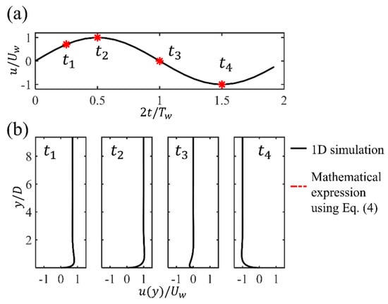
Figure 2. (a) The time series of free-stream velocity for $\mathrm{K}\mathrm{C}=400$ and $k_s/D=0.05$, where four representative phases at $2t_1/T_w=0.25$, $2t_2/T_w=0.5$, $2t_3/T_w=1.0$,$2t_4/T_w=1.5$ are indicated. (b) The corresponding vertical profiles of the horizontal velocity obtained by the 1D simulations at the four phases.

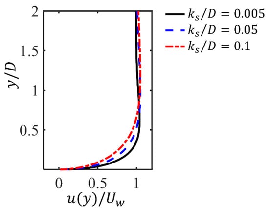
Figure 3. The vertical profiles of the horizontal velocity at the peak value for $\mathrm{K}\mathrm{C}=400$ and different $k_s/D$.

To determine the optimal grid resolution, the mesh convergence study is performed for the wall-mounted case at $\mathrm{K}\mathrm{C}=400$ and $k_s/D=0.005$. Three computational meshes from coarse to dense are generated using the utility. The grid number for the three meshes are Mesh 1: 10,084; Mesh 2: 17,238 and Mesh 3: 28,280. The time-step for all meshes is $∆t=1\times {10}^{-3}$ to keep the maximum Courant number below 0.4. Figure 4 shows the time histories of the drag force coefficient $C_x=F_x/(0.5\rho D{L}_z{U}_w^2)$ and the lift force coefficient $C_y=F_y/(0.5\rho D{L}_z{U}_w^2)$ of the cylinder for different meshes. For the two forces, $F_x$ and $F_y$ are the horizontal and vertical forces acting on the cylinder and $L_z$ is the spanwise length. When the mesh number increases from Mesh 2 to Mesh 3, the temporal evolutions of $C_x$ and $C_y$ for the two meshes are almost the same except for slight differences at the peak values for the two time series. The value of the peak value of $C_x$ ($C_{x,max}$), the time-averaged $C_y$ ($\overline{C_y}$) and the peak value of $C_y$ ($C_{y,max}$) for each mesh are shown in Table 2. It can be seen that the relative difference of $C_{x,max}$ reduces to below 5% between Meshes 2 and 3. The relative differences of $\overline{C_y}$ are all less than 5% between two consecutive meshes. The relative differences of $C_{y,max}$ can be up to 13% between Meshes 2 and 3 due to the sensitivity of the $C_y$ value. In general, Mesh 3 can provide sufficient grid resolutions to predict the hydrodynamic forces and the grid resolution is used for all investigated cases. To further quantify the mesh convergence study, the Grid Convergence Index (GCI) method proposed by [41] is computed. First, the averaged grid size, defined as $h_g=\left({\sum }_i^N∆V_i\right)/N$ ($∆V_i$ is the volume of each cell and $N$ is the total grid number), is used to represent the global characteristics of the three meshes. For the present study, the grid refinement factor $r=h_{coarse}/h_{fine}$ for the three meshes are all larger than 1.3, which can be regarded as desirable according to [41]. Take the peak drag coefficient $C_{x,max}$ in the present study for example, the apparent order $P$ can be determined by iteratively solving the nonlinear equations of

$$P={\displaystyle \frac{1}{ln\left(r_{32}\right)}}\left|ln{\displaystyle \frac{{\epsilon }_{21}}{{\epsilon }_{32}}}+q\left(P\right)\right|$$

(9a)

$$q\left(P\right)=\mathit{ln}{\displaystyle \frac{r_{32}^P-s}{r_{21}^P-s}}$$

(9b)

where ${\epsilon }_{21}=C_{x,max,Mesh2}-C_{x,max,Mesh1}$ and ${\epsilon }_{32}=C_{x,max,Mesh3}-C_{x,max,Mesh2}$.

Also, $r_{21}=h_{g,Mesh2}/h_{g,Mesh1}$, $r_{32}=h_{g,Mesh3}/h_{g,Mesh2}$ and $s=\mathrm{s}\mathrm{i}\mathrm{g}\mathrm{n}({\epsilon }_{21}/{\epsilon }_{32})$. Then, the exact extrapolated value of $C_{x,max}$ with a grid size of $h_g=0$ can be estimated as $C_{x,max,ext}=(r_{32}^P{C}_{x,max,Mesh3}-C_{x,max,Mesh2})/(r_{32}^P-1)=1.33$. The grid convergence index (GCI), used as an indicator of the mesh convergence study, is calculated as ${GCI}^{21}=1.25e_a^{21}/(r_{21}^P-1)=1.9\%$ and ${GCI}^{32}=1.25e_a^{32}/(r_{32}^P-1)=0.09\%$ with the relative error between meshes $e_a^{21}=\left|(C_{x,max,Mesh2}-C_{x,max,Mesh1})/C_{x,max,Mesh2}\right|$ and $e_a^{32}$ in a similar manner. It can be seen that the GCI value on the finest grid for the maximum $C_{x,max}$ was below 1%, suggesting that the numerical uncertainty introduced by the spatial discretization is low for the peak drag value prediction.

The time series of the averaged $y^{+}$ (defined as ${\displaystyle \frac{{∆yu}_{\ast }}{\nu }},$ where $∆y$ is the distance of the first near-wall grid points to the wall surface) on the bottom-wall and cylinder surface for the three meshes are also shown in Figure 4c,d. It can be seen that for the adopted Mesh 3, the $y^{+}$ value on both the cylinder surface and the bottom-wall is less than 1. Since the wall function is employed in the present study, the near-wall boundary layer can be well modeled with $y^{+}\lesssim 1$. The validation of the present numerical model is reported in [20] and is not repeated here. In addition, the presently employed $k-\omega$ Shear Stress Transport (SST) turbulent model was also used and validated in [25].

Figure 4. The time series of (a) $C_x$, (b) $C_y$, the $y^{+}$ values on (c) the cylinder surface and (d) the bottom-wall for different meshes for the wall-mounted case at $\mathrm{K}\mathrm{C}=400$ and $k_s/D=0.005$.

Table 2. Mesh numbers and hydrodynamic force coefficients for different meshes.

Mesh	Mesh No.	${\mathit{C}}_{\mathit{x},\mathit{m}\mathit{a}\mathit{x}}$	$\overline{{\mathit{C}}_{\mathit{y}}}$	${\mathit{C}}_{\mathit{y},\mathit{m}\mathit{a}\mathit{x}}$
1	10,084	0.812	0.3	0.854
2	17,238	1.35	0.29	0.937
3	28,280	1.33	0.28	0.824

Table 2. Mesh numbers and hydrodynamic force coefficients for different meshes.

Mesh	Mesh No.	${\mathit{C}}_{\mathit{x},\mathit{m}\mathit{a}\mathit{x}}$	$\overline{{\mathit{C}}_{\mathit{y}}}$	${\mathit{C}}_{\mathit{y},\mathit{m}\mathit{a}\mathit{x}}$
1	10,084	0.812	0.3	0.854
2	17,238	1.35	0.29	0.937
3	28,280	1.33	0.28	0.824

3. Results and Discussion

3.1. Hydrodynamic Force Coefficients

The time histories of the drag and lift force coefficients for Cases 1 to 9 for the three investigated $\mathrm{K}\mathrm{C}$s and different $k_s/D$s are displayed in Figure 5. A regular oscillatory pattern is observed for the time series of the force coefficients. At the largest $\mathrm{K}\mathrm{C}=400$, an overall symmetry behavior is shown for $C_x$ with respect to the zero value, despite there being strong spikes in the positive direction along with a secondary peak after the spike while the spikes in the negative direction are relatively weaker. A detailed inspection of the time series comparing the horizontal velocity value at the cylinder center with $C_x$ and $C_y$ is shown for $\mathrm{K}\mathrm{C}=400$ and $k_s/D=0.1$ in Figure 6. It can be seen that the spikes happen closely after the flow becomes reversed from in the negative direction to the positive direction. The second peaks after the spike in the $C_x$ and $C_y$ correspond to the peak value of the flow velocity. This asymmetry in the $C_x$ time series may be related to the initial phase of the oscillatory boundary layer. Although the inlet velocity profiles represent a fully developed boundary layer, the initial flow phase may still introduce slight asymmetries. Especially in the early-stage wave cycles, there is transient adjustment of the flow field around the cylinder. These early asymmetries can persist and accumulate, which influences the time series of the drag force. In addition, in the wall-mounted cylinder configurations and the configurations with a small gap ratio, the flows around the lower corner of the cylinder and through the gap between the cylinder and the seabed can be highly sensitive to small variations in incoming flow velocity and pressure gradients. This sensitivity may result in unbalanced shear layer development on either side of the cylinder, particularly during flow reversal. These flow features may lead to asymmetry in the drag coefficient over the wave cycle. These spikes are also observed at $\mathrm{K}\mathrm{C}=200$ and seem to be merged as a single peak value during each cycle at $\mathrm{K}\mathrm{C}=20$. For the lift coefficient $C_y$, there are multiple peaks during one cycle for large $\mathrm{K}\mathrm{C}=200$ and 400, indicating that although the vortex shedding is suppressed for these wall-mounted cases, there is still an unsteady characteristic, which may be due to the movement and flapping of the shear layer over the cylinder. For the small $\mathrm{K}\mathrm{C}=20$, regular and close to sinusoidal behavior is shown for $C_y$. For different $k_s/D$ s, there are slight phase differences in the peaks of $C_x$ and $C_y$ depending on the different vertical phase difference in the oscillatory boundary layers at the large $\mathrm{K}\mathrm{C}=400$ and 200. At $\mathrm{K}\mathrm{C}=400$, the difference in the first peak for different $k_s/D$ is not significant, while there is an apparent decrease in the second peak, as shown in the zoom-in figure around the peak values in Figure 7. Also, with the increasing $\mathrm{K}\mathrm{C}$, the boundary layer effects become significant, leading to an increasing velocity reduction with the increasing $k_s/D$. Therefore, there is a decrease in the force coefficients, especially in the root-mean-square values of $C_x,$ for large $k_s/D$, as shown in Figure 8a. For the root-mean-square values of $C_y$ at $\mathrm{K}\mathrm{C}=400$ and 200, the decrease is obvious, with $k_s/D$ increasing from 0.005 to 0.5 while becoming constant from $k_s/D=0.05$ to 0.1, as shown in Figure 8b. However, for the small $\mathrm{K}\mathrm{C}=20$, the inertial effects of the oscillatory flow are dominant and there is almost no difference in $C_x$ and $C_y$ for different $k_s/D$.

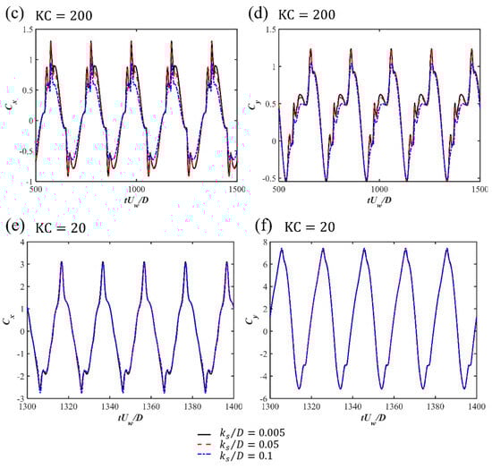
Figure 5. The time histories of the drag force coefficients $C_x$ (a,c,e) and lift force coefficients $C_y$ (b,d,f) for the wall-mounted cases at different $\mathrm{K}\mathrm{C}$.

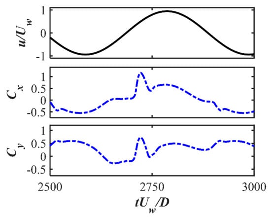
Figure 6. The horizontal velocity of the oscillatory boundary layer at the cylinder center and the time series of $C_x$ and $C_y$ for $\mathrm{K}\mathrm{C}=400$ and $k_s/D=0.1$.

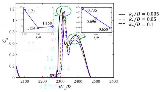
Figure 7. A zoomed-in figure of the time series around the peak drag coefficient in Figure 5a for the wall-mounted case at $\mathrm{K}\mathrm{C}=400$.

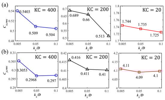
Figure 8. The root-mean-square values of (a) $C_x$ and (b) $C_y$ for the wall-mounted cases with different $\mathrm{K}\mathrm{C}$.

The time histories of the drag and lift force coefficients for Cases 10 to 12 at $\mathrm{K}\mathrm{C}=400$ and $k_s/D=0.05$ for different $G/D$s are shown in Figure 9 to evaluate the influences of the gap ratio. It demonstrates that the amplitude of $C_x$ monotonically increases with the increasing $G/D$. There is significant decrease in the $C_y$ amplitude from the wall-mounted case to the $G/D=0.05$ case, while with the further increasing $G/D$, the net $C_y$ decreases with an increasing oscillation amplitude. The oscillation behavior is due to the vortex shedding during one oscillatory flow cycle for the high $\mathrm{K}\mathrm{C}$ value, which has also been reported in [20].

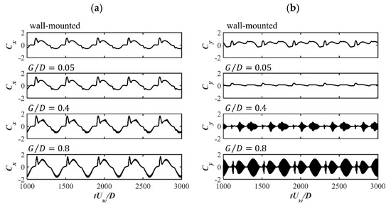
Figure 9. The time histories of (a) $C_x$ and (b) $C_y$ for $\mathrm{K}\mathrm{C}=400$, $k_s/D=0.05$ and different $G/D$s.

3.2. Flow Fields

The spanwise vorticity at different time steps during one oscillation period is shown in Figure 10. At the peak points of the drag force shown in Figure 10a,d, the shear layer separated from the upper surface is stretched to its largest length, which also corresponds to the peak values of the lift force. Depending on the phase of the initial condition, there is an attachment of the upstream bottom-wall boundary layer on the front surface of the cylinder and this may enhance the separated shear layer from the cylinder, as shown in Figure 10a,c. Then, the shear layer from the upper surface is bent and begins to attach the bottom wall. This results in the second positive peak in the drag force series, shown in Figure 10e. Then, the oscillatory flow starts to reverse, and the strength of the shear layer becomes weaker.

Furthermore, to quantify the contribution of the surrounding flow to the hydrodynamic forces, the contours of the force element $F_{x,\mathbf{u}\times \mathsf{\omega }}/U_w^2$ and $F_{y,\mathbf{u}\times \mathsf{\omega }}/U_w^2$ at the time steps in Figure 10a,d,e, corresponding to the peak values of the forces, are shown in Figure 11. This analysis can reveal the correlations between the forces and coherent flow structures without integrating the pressure on the cylinder surface, which is different from the approaches of previous studies such as [23,25]. It should be noted that it is the volume integral of the contours over the entire computational domain that contributes to the total drag and lift force. However, the contours can still identify critical regions in the flow fields making the dominant contributions to the drag and lift forces. It can be seen that both the front edge of the cylinder and the shear layer region contribute to the drag force but the $F_{x,\mathbf{u}\times \mathsf{\omega }}/U_w^2$ values of two regions are opposite. At the time steps of Figure 11a,c, the $F_{x,\mathbf{u}\times \mathsf{\omega }}/U_w^2$ structures are almost antisymmetric with respect to the cylinder and the opposite contributions around the front edges of the cylinder are attenuated for these two time steps. At the drag force peak seen in Figure 11b, both regions reach their highest values. The front edge region seems to be enhanced by the attachment of the bottom-wall boundary layer and the shear layer is also strengthened and elongated. For the $F_{y,\mathbf{u}\times \mathsf{\omega }}/U_w^2$ values, the primary contributions originate from the front edges of the cylinder and the peak region in Figure 11d is related to the enhancement of the cylinder front edge, as shown in Figure 11e. The drag force element $F_{x,\mathbf{u}\times \mathsf{\omega }}/U_w^2$ can be further decomposed into contributions from the horizontal and vertical velocity, respectively: $F_{x,v{\omega }_z}/U_w^2=\int \left(v{\omega }_z\right)·\left(\partial {\varphi }_x/\partial x\right)\mathrm{d}V/U_w^2$ and $F_{x,u{\omega }_z}/U_w^2=\int -\left(u{\omega }_z\right)·\left(\partial {\varphi }_x/\partial y\right)\mathrm{d}V/U_w^2$. The time series of the two drag elements during one cycle are shown in Figure 12, which shows that the contributions from the two velocity components to the total drag forces are almost the same. The contours of $F_{x,v}/U_w^2$ and $F_{x,u{\omega }_z}/U_w^2$ at the two peak time steps shown in Figure 10d,e are displayed in Figure 12a–d, respectively. It can be seen that around the front upper corner of the cylinder, although the strength of ${\omega }_z$ is weak, there is high vertical velocity around this region, which contributes to the positive peak of the drag forces. For the force element $F_{x,u{\omega }_z}/U_w^2$, related to the horizontal velocity, the primary positive contribution is from the shear layer region, with high amplitudes of both ${\omega }_z$ and $u$.

Figure 10. The contours of the spanwise vorticity at different time steps for the wall-mounted cylinder at $\mathrm{K}\mathrm{C}=400$ and $k_s/D=0.1$. Each figure corresponds to the time step denoted by the red star in the time series of $C_x$ and $C_y$ (a–f).

Figure 11. The contours of the force elements of the drag $F_{x,\mathbf{u}\times \mathsf{\omega }}/U_w^2$ (a–c) and lift forces $F_{y,\mathbf{u}\times \mathsf{\omega }}/U_w^2$ (d–f) at different time steps for the wall-mounted cylinder at $\mathrm{K}\mathrm{C}=400$ and $k_s/D=0.1$. Each figure corresponds to the time step denoted by the red star in the time series of $C_x$ and $C_y$.

Figure 12. The contours of the force elements associated with (a,c) the vertical velocity component $F_{x,v{\omega }_z}/U_w^2$ and (b,d) the horizontal velocity component $F_{x,u{\omega }_z}/U_w^2$ at the two time steps of the peak drag force coefficients for the wall-mounted cylinder at $\mathrm{K}\mathrm{C}=400$ and $k_s/D=0.1$. Each figure corresponds to the time step denoted by the red star in the time series of $C_x$.

To visualize the influences of the bottom-wall roughness, the spanwise vorticities at the two peak points, as denoted in Figure 10d,e for the wall-mounted cases at $\mathrm{K}\mathrm{C}=400$, are shown in Figure 13. An increasing velocity reduction can be observed from the weakened velocity gradient at the bottom-wall boundary layer with the increasing roughness. At the first peak point, the enhancement of the shear layer separated from the upper surface of the cylinder by the bottom-wall boundary layer is the strongest, with the lowest $k_s/D=0.005$, which may result in the highest drag force for this case, as shown in Figure 5a. The velocity reduction also leads to the weakened shear layer at the second peak point, as shown in Figure 13b,d,f. With the increasing $k_s/D$, the shear layer from the cylinder tends to be further attached to the bottom wall.

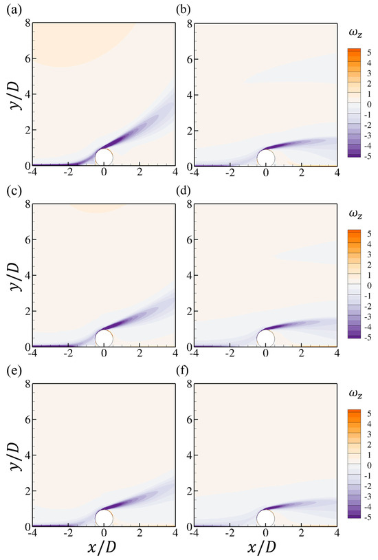
Figure 13. The contours of the spanwise vorticity at two peak values of $C_x,$ shown in Figure 10d,e, for different $k_s/D$: (a,b) $k_s/D=0.005$; (c,d) $k_s/D=0.05$ and (e,f) $k_s/D=0.1$.

To evaluate the influences of $\mathrm{K}\mathrm{C}$, the flow fields at two smaller $\mathrm{K}\mathrm{C}=200$ and $\mathrm{K}\mathrm{C}=20$ are shown for $k_s/D=0.1$ and wall-mounted cases. The contours of the spanwise vorticity at several critical time steps during one cycle of the drag force are shown in Figure 14 and Figure 15. The $\mathrm{K}\mathrm{C}=200$ case is still characterized by an elongated shear layer separated from the top surface of the cylinder, while the strength and length of the shear layer are both lower than that at $\mathrm{K}\mathrm{C}=400$. At the peak value of the drag force in Figure 14c, the shear layer already becomes attached to the bottom wall, which is different from the $\mathrm{K}\mathrm{C}=400$ case. For the $\mathrm{K}\mathrm{C}=20$ case, the flow patterns are significantly different from the large $\mathrm{K}\mathrm{C}$ cases. It is obvious that there is no shear layer stretching and elongation. At the negative peak of the drag force in Figure 15a, the shear layer is rolled up and then pushed back by the reverse flow, which is also accompanied by the attachment of the bottom boundary layer to the cylinder, as shown in Figure 15b. The attached bottom boundary layer also breaks the shear layer in Figure 15c and the separated vortex is washed back with the oscillatory flow, which forms a vortex pair, as shown in Figure 15a,d.

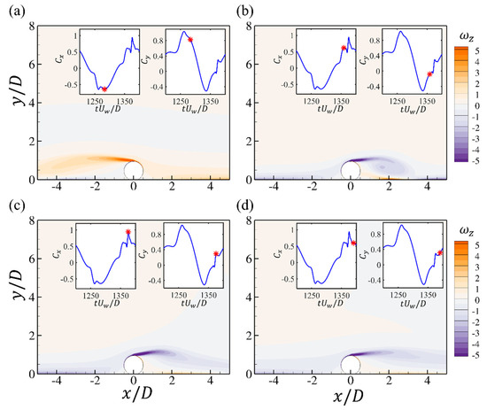
Figure 14. The contours of the spanwise vorticity at different time steps for the wall-mounted cylinder at $\mathrm{K}\mathrm{C}=200$ and $k_s/D=0.1$. Each figure corresponds to the time step denoted by the red star in the time series of $C_x$ and $C_y$ (a–d).

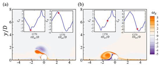
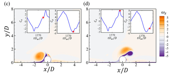
Figure 15. The contours of the spanwise vorticity at different time steps for the wall-mounted cylinder at $\mathrm{K}\mathrm{C}=20$ and $k_s/D=0.1$. Each figure corresponds to the time step denoted by the red star in the time series of $C_x$ and $C_y$(a–d).

To quantify the overall time-varying flow patterns with different $G/D$ and their correlation with the hydrodynamic forces, the spanwise vorticity at three critical time steps during one oscillation period and the corresponding force elements of $F_{x,\mathit{u}\times \mathit{\omega }}/U_w^2$ and $F_{y,\mathit{u}\times \mathit{\omega }}/U_w^2$ for $\mathrm{K}\mathrm{C}=400$ and $k_s/D=0.05$ are shown in Figure 16. For a small gap of $G/D=0.05$, it can be seen from Figure 16 that the vortex shedding is suppressed and there is only slow movement of the long shear layer separated from the cylinder surface. A fast jet flow passes through the small gap between the cylinder and the bottom wall and induces two strong shear layers from the two boundaries. Both of the two shear layers seem to be attached to the cylinder after flowing after the gap. At the two negative and positive peaks of the drag force in Figure 16a,c, the flow patterns are antisymmetric with respect to the cylinder. Based on the contours of $F_{x,\mathit{u}\times \mathit{\omega }}/U_w^2$, the main contribution is from the shear layers from the surface of the cylinder while the tilted shear layer from the bottom wall makes reverse contributions, as shown in Figure 16d,f. At the peak value of the drag in Figure 16b, the stretching of the upper shear layer is similar to the wall-mounted case. For the drag element $F_{x,\mathit{u}\times \mathit{\omega }}/U_w^2$ in Figure 16e, it can be seen that the drag contribution from the upper part of the cylinder is also similar to that of the wall-mounted case shown in Figure 11b. The drag force elements from the lower shear layer of the cylinder and the bottom wall are opposite, which makes an almost zero net contribution to the total drag force. Therefore, the total drag forces for the $G/D=0.05$ case and the wall-mounted case are almost similar. Furthermore, the jet flow through the small gap makes a positive contribution to the lift force but is compensated by the large negative contribution of the lower shear layer of the cylinder, leading to a smaller lift force compared with the wall-mounted case.

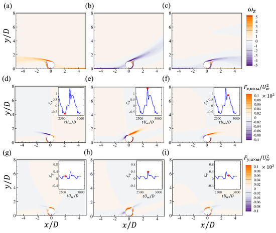
Figure 16. The contours of the spanwise vorticity (a–c); the force elements of the drag $F_{x,\mathit{u}\times \mathit{\omega }}/U_w^2$ (d–f) and lift forces $F_{y,\mathit{u}\times \mathit{\omega }}/U_w^2$ (g–i) at different time steps for the wall-mounted cylinder at $\mathrm{K}\mathrm{C}=400$, $k_s/D=0.05$ and $G/D=0.05$. Each figure corresponds to the time step denoted by the red star in the time series of $C_x$ and $C_y$.

The spanwise vorticity at three critical time steps during one oscillation period for $\mathrm{K}\mathrm{C}=400$, $k_s/D=0.05$ and $G/D=0.4$ is shown in Figure 17. It can be seen that there is vortex shedding around the negative peak of the drag force shown in Figure 17a. In addition, the separation of the shear layer from the lower surface of the cylinder also induces the separation of the bottom-wall boundary layer, which forms a vortex pair in the further downstream region, as denoted in Figure 17a. The contours of the drag force element $F_{x,\mathit{u}\times \mathit{\omega }}/U_w^2$ shows that both the shear layers from the upper and lower surfaces of the cylinder make the dominant contribution to the drag force. For the lift force element $F_{y,\mathit{u}\times \mathit{\omega }}/U_w^2$, it can be seen that the shear layers from the upper and lower surfaces make opposite contributions to the lift force. When the shear layer begins to separate, its contribution to the lift force becomes reversed. There are both positive and negative regions in the contours of $F_{y,\mathit{u}\times \mathit{\omega }}/U_w^2$ when the shear layer is rolled up, as shown in Figure 17g,i. The positive peak value of the drag force corresponds to the expansion and extension of the two shear layers in the streamwise direction, as shown in Figure 17b when the boundary layer flow begins to reach its maximum value. The elongated shear layers from both upper and lower parts of the cylinder significantly contribute to the drag force, as shown by the $F_{x,\mathit{u}\times \mathit{\omega }}/U_w^2$ contours.

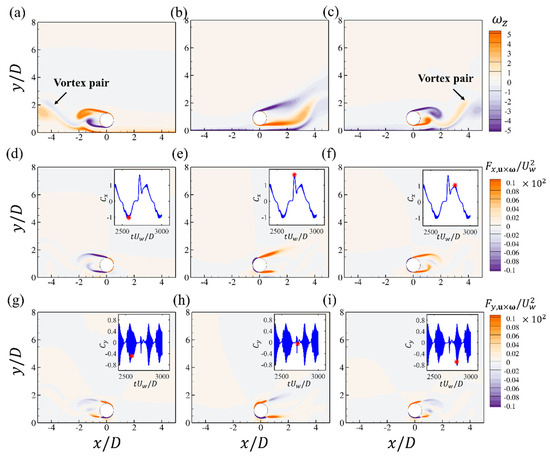
Figure 17. The contours of the spanwise vorticity (a–c); the force elements of the drag $F_{x,\mathbf{u}\times \mathsf{\omega }}/U_w^2$ (d–f) and lift forces $F_{y,\mathbf{u}\times \mathsf{\omega }}/U_w^2$ (g–i) at different time steps for the wall-mounted cylinder at $\mathrm{K}\mathrm{C}=400$, $k_s/D=0.05$ and $G/D=0.4$. Each figure corresponds to the time step denoted by the red star in the time series of $C_x$ and $C_y$.

The spanwise vorticity at three critical time steps during one oscillation period for $\mathrm{K}\mathrm{C}=400$, $k_s/D=0.05$ and $G/D=0.8$ is shown in Figure 18. The vortex shedding around the negative peak and the second positive peak of the drag force is similar to that of the current flow past a cylinder, as shown in Figure 18a,c. Even at the spike of the drag force shown in Figure 18b, the overall wake flow is also similar to that in Figure 18c, except that there seems to be a slight expansion of the two shear layers in the streamwise direction, which may be enhanced by the bottom-wall boundary layer when it is reversed. Due to the expansion of the shear layer, the volume integral of the drag force element $F_{x,\mathit{u}\times \mathit{\omega }}/U_w^2$ is also larger than that in Figure 18c. The distributions of the lift force element $F_{y,\mathit{u}\times \mathit{\omega }}/U_w^2$ around the cylinder are also similar for the $G/D=0.4$ case.

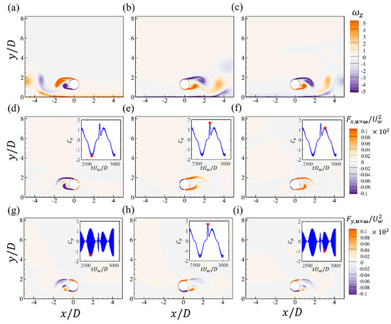
Figure 18. The contours of the spanwise vorticity (a–c); the force elements of the drag $F_{x,\mathbf{u}\times \mathsf{\omega }}/U_w^2$ (d–f) and lift forces $F_{y,\mathbf{u}\times \mathsf{\omega }}/U_w^2$ (g–i) at different time steps for the wall-mounted cylinder at $\mathrm{K}\mathrm{C}=400$, $k_s/D=0.05$ and $G/D=0.8$. Each figure corresponds to the time step denoted by the red star in the time series of $C_x$ and $C_y$.

4. Conclusions

Numerical simulations are performed to investigate the hydrodynamic forces on a wall-mounted cylinder and a near-wall cylinder with a rough seabed. The correlations between the hydrodynamic characteristics and the surrounding flow characteristics around the cylinder are revealed through the force partitioning method (FPM). The RANS simulation is combined with the k–ω SST turbulence model to resolve the turbulent stress and the wall function is used to represent the seabed roughness. The time-varying wave-induced oscillatory boundary layer velocity profile obtained from additional 1D simulations is prescribed at the inlet of the computational domain. The influences of different KC and seabed roughness on the flow characteristics and hydrodynamic characteristics are discussed. The main conclusions from the numerical simulations are outlined as follows:

• There are strong spikes in the drag and lift force time series for the wall-mounted cylinder, which occur closely after the main flow direction is reversed, followed by second peaks corresponding to the peak value of the main flow velocity.
• With the increasing $k_s/D$, the boundary layer effects become significant for the large $\mathrm{K}\mathrm{C}$, leading to an increasing velocity reduction and decreasing peak values of the force coefficients. For the small $\mathrm{K}\mathrm{C}$, the inertial effect from the oscillatory flow dominates the oscillatory behavior of the force coefficients, leading to an insignificant difference in $C_x$ and $C_y$ for different $k_s/D$.
• With the increasing gap ratio, the net lift coefficient starts to decrease and there is vortex shedding for the large KC cases, which results in an additional high-frequency oscillation in the time-series of the lift coefficient.
• The FPM analysis reveals that for the wall-mounted cases, the elongated shear layers from the top of the cylinder contribute to the peak values of the drag force coefficients. The spikes of the coefficients may be related to the enhancement of the shear layer by the reversed bottom boundary layer flows. For the cases with a small gap ratio to the bottom wall, the jet flows through the gap contribute to the lift forces. In addition, the contributions of the shear layers to the lift forces become reversed when they become elongated and separated.

It is worth highlighting that the FPM analysis enables the quantification of hydrodynamic forces on the cylinder using only the surrounding flow velocity data, without the need for pressure measurements on the cylinder surface. This may provide a practical and non-intrusive methodology for evaluating hydrodynamic loads on near-seabed pipelines under oscillatory coastal flow conditions, which can significantly aid in the design and stability assessment of coastal infrastructures. Other environmental factors such as temperature gradients and background ocean currents will also influence near-seabed boundary layer flows and hydrodynamic loads on pipelines and cables. These effects are not considered in the present study but will be investigated in future work.

References

- Teng, Y.; Griffiths, T.; An, H.; Draper, S.; Tang, G.; Mohr, H.; White, D.J.; Fogliani, A.; Cheng, L. Hydrodynamic forces on subsea cables immersed in wave boundary layers. Coast. Eng. 2022, 174, 104101. [Google Scholar] [CrossRef]
- Reda, A.; Low, H.E.; Shahin, M.A. Surface Roughness Analysis of Subsea Cables/Umbilicals. J. Mar. Sci. Eng. 2025, 13, 111. [Google Scholar] [CrossRef]
- Yang, S.H.; Ringsberg, J.W.; Johnson, E. Parametric study of the dynamic motions and mechanical characteristics of power cables for wave energy converters. J. Mar. Sci. Technol. 2018, 23, 10–29. [Google Scholar] [CrossRef]
- Jin, H. Design and construction of a large-diameter crude oil pipeline in Northeastern China: A special issue on permafrost pipeline. Cold Reg. Sci. Technol. 2010, 64, 209–212. [Google Scholar] [CrossRef]
- Stansby, P.K. Forces on a circular cylinder in elliptical orbital flows at low Keulegan-Carpenter numbers. Appl. Ocean Res. 1993, 15, 281–292. [Google Scholar] [CrossRef]
- Griffiths, T.; Teng, Y.; Cheng, L.; An, H.; Draper, S.; Mohr, H.; Fogliani, A.; Mariani, A.; White, D. Hydrodynamic forces on near-bed small diameter cables and pipelines in currents waves and combined flow. In Proceedings of the International Conference on Offshore Mechanics and Arctic Engineering, Glasgow, UK, 9–14 June 2019; American Society of Mechanical Engineers: New York, NY, USA; Volume 58813, p. V05BT04A019. [Google Scholar]
- Yuan, Z.; Huang, Z. Morison coefficients for a circular cylinder oscillating with dual frequency in still water: An analysis using independent-flow form of Morison’s equation. J. Ocean Eng. Mar. Energy 2015, 1, 435–444. [Google Scholar] [CrossRef]
- Petersen, T.U.; Mandviwalla, X.; Christensen, E.D.; Tarp-Johansen, N.J.; Rüdinger, F. Oscillatory loads on circular cylinder with secondary structures. J. Fluids Struct. 2020, 94, 102935. [Google Scholar] [CrossRef]
- Ren, C.; Lu, L.; Cheng, L.; Chen, T. Hydrodynamic damping of an oscillating cylinder at small Keulegan—Carpenter numbers. J. Fluid Mech. 2021, 913, A36. [Google Scholar] [CrossRef]
- Chang, W.Y.; Constantinescu, G. Oscillatory flow around a vertical circular cylinder placed in an open channel: Coherent structures, sediment entrainment potential and drag forces. J. Fluid Mech. 2023, 964, A22. [Google Scholar] [CrossRef]
- Tong, F.; Cheng, L.; Zhao, M.; An, H. Oscillatory flow regimes around four cylinders in a square arrangement under small conditions. J. Fluid Mech. 2015, 769, 298–336. [Google Scholar] [CrossRef]
- Sumer, B.M.; Jensen, B.L.; Fredsøe, J. Effect of a plane boundary on oscillatory flow around a circular cylinder. J. Fluid Mech. 1991, 225, 271–300. [Google Scholar] [CrossRef]
- An, H.; Cheng, L.; Zhao, M. Steady streaming around a circular cylinder near a plane boundary due to oscillatory flow. J. Hydraul. Eng. 2011, 137, 23–33. [Google Scholar] [CrossRef]
- Fuhrman, D.R.; Baykal, C.; Sumer, B.M.; Jacobsen, N.G.; Fredsøe, J. Numerical simulation of wave-induced scour and backfilling processes beneath submarine pipelines. Coast. Eng. 2014, 94, 10–22. [Google Scholar] [CrossRef]
- Larsen, B.E.; Fuhrman, D.R.; Sumer, B.M. Simulation of wave-plus-current scour beneath submarine pipelines. J. Waterw. Port Coast. Ocean Eng. 2016, 142, 04016003. [Google Scholar] [CrossRef]
- Huang, J.; Yin, G.; Ong, M.C.; Myrhaug, D.; Jia, X. Numerical investigation of scour beneath pipelines subjected to an oscillatory flow condition. J. Mar. Sci. Eng. 2021, 9, 1102. [Google Scholar] [CrossRef]
- Sun, S.; Yang, W.; Liu, S.; Li, P.; Ong, M.C. Computational fluid dynamics simulations of a near-wall rectangular cylinder in an oscillatory flow. Ocean Eng. 2024, 304, 117776. [Google Scholar] [CrossRef]
- Cheng, L.; An, H.; Draper, S.; White, D. Effect of wave boundary layer on hydrodynamic forces on small diameter pipelines. Ocean Eng. 2016, 125, 26–30. [Google Scholar] [CrossRef]
- Tang, G.; Cheng, L.; Lu, L.; Teng, Y.; Zhao, M.; An, H. Effect of oscillatory boundary layer on hydrodynamic forces on pipelines. Coast. Eng. 2018, 140, 114–123. [Google Scholar] [CrossRef]
- Yin, G.; Ong, M.C.; Ye, N. Hydrodynamic Forces on a Near-Bottom Pipeline Subject to Wave-Induced Boundary Layer. J. Offshore Mech. Arct. Eng. 2024, 146, 021803. [Google Scholar] [CrossRef]
- Menter, F.R. Two-equation eddy-viscosity turbulence models for engineering applications. AIAA J. 1994, 32, 1598–1605. [Google Scholar] [CrossRef]
- Zhao, M.; Cheng, L.; Teng, B.; Dong, G. Hydrodynamic forces on dual cylinders of different diameters in steady currents. J. Fluids Struct. 2007, 23, 59–83. [Google Scholar] [CrossRef]
- Jiang, H.; Cheng, L. Numerical modeling of turbulent wall-bounded oscillatory flow and its effect on small-diameter pipelines. In Proceedings of the International Conference on Offshore Mechanics and Arctic Engineering, Online, 3–7 August 2020; American Society of Mechanical Engineers: New York, NY, USA; Volume 84409, p. V008T08A034. [Google Scholar] [CrossRef]
- Jang, H.K.; Ozdemir, C.E.; Liang, J.H.; Tyagi, M. Oscillatory flow around a vertical wall-mounted cylinder: Flow pattern details. Phys. Fluids 2021, 33, 025114. [Google Scholar] [CrossRef]
- Jiang, H.; Teng, Y.; Cheng, L.; Draper, S.; An, H. Symmetric oscillatory flow induces asymmetric lift on a bottom-mounted horizontal cylinder. Phys. Fluids 2025, 37, 025171. [Google Scholar] [CrossRef]
- Jiang, H.; Cheng, L.; He, F.; Guo, Z.; Cai, Y.; Cen, Z.; Wang, L. Wall boundary conditions for RANS modelling of unidirectional and oscillatory boundary-layer flows. Ocean Eng. 2024, 312, 119175. [Google Scholar] [CrossRef]
- Spalding, D.B. A single formula for the law of the wall. J. Appl. Mech. 1961, 28, 455–458. [Google Scholar] [CrossRef]
- Wilcox, D.C. Formulation of the kw turbulence model revisited. AIAA J. 2008, 46, 2823–2838. [Google Scholar] [CrossRef]
- Nagel, T. Numerical Study of Multi-Scale Flow-Sediment-Structure Interactions Using a Multiphase Approach. Ph.D. Thesis, Université Grenoble Alpes, Grenoble, France, 2018. [Google Scholar]
- Chang, C.C. Potential flow and forces for incompressible viscous flow. Proceedings of the Royal Society of London. Ser. A Math. Phys. Sci. 1992, 437, 517–525. [Google Scholar]
- Zhang, K.; Hayostek, S.; Amitay, M.; He, W.; Theofilis, V.; Taira, K. On the formation of three-dimensional separated flows over wings under tip effects. J. Fluid Mech. 2020, 895, A9. [Google Scholar] [CrossRef]
- Menon, K.; Mittal, R. Significance of the strain-dominated region around a vortex on induced aerodynamic loads. J. Fluid Mech. 2021, 918, R3. [Google Scholar] [CrossRef]
- Menon, K.; Mittal, R. On the initiation and sustenance of flow-induced vibration of cylinders: Insights from force partitioning. J. Fluid Mech. 2020, 907, A37. [Google Scholar] [CrossRef]
- Yin, G.; Janocha, M.J.; Ong, M.C. Estimation of hydrodynamic forces on cylinders undergoing flow-induced vibrations based on modal analysis. J. Offshore Mech. Arct. Eng. 2022, 144, 060904. [Google Scholar] [CrossRef]
- Aghaei-Jouybari, M.; Seo, J.H.; Yuan, J.; Mittal, R.; Meneveau, C. Contributions to pressure drag in rough-wall turbulent flows: Insights from force partitioning. Phys. Rev. Fluids 2022, 7, 084602. [Google Scholar] [CrossRef]
- VimalKumar, S.; De Tavernier, D.; von Terzi, D.; Belloli, M.; Viré, A. Force-partitioning analysis of vortex-induced vibrations of wind turbine tower sections. Wind Energy Sci. 2024, 9, 1967–1983. [Google Scholar] [CrossRef]
- Kumar, P.; Singh, S.K. Flow past a bluff body subjected to lower subcritical Reynolds number. J. Ocean Eng. Sci. 2020, 5, 173–179. [Google Scholar] [CrossRef]
- Schewe, G.; van Hinsberg, N.P.; Jacobs, M. Investigation of the steady and unsteady forces acting on a pair of circular cylinders in crossflow up to ultra-high Reynolds numbers. Exp. Fluids 2021, 62, 176. [Google Scholar] [CrossRef]
- Kološ, I.; Michalcová, V.; Lausová, L. Numerical analysis of flow around a cylinder in critical and subcritical regime. Sustainability 2021, 13, 2048. [Google Scholar] [CrossRef]
- Cao, Y.; Tamura, T. Large-eddy simulation study of Reynolds number effects on the flow around a wall-mounted hemisphere in a boundary layer. Phys. Fluids 2020, 32, 025109. [Google Scholar] [CrossRef]
- Celik, I.B.; Ghia, U.; Roache, P.J.; Freitas, C.J. Procedure for estimation and reporting of uncertainty due to discretization in CFD applications. J. Fluids Eng.-Trans. ASME 2008, 130, 078001. [Google Scholar] [CrossRef]
Disclaimer/Publisher’s Note: The statements, opinions and data contained in all publications are solely those of the individual author(s) and contributor(s) and not of MDPI and/or the editor(s). MDPI and/or the editor(s) disclaim responsibility for any injury to people or property resulting from any ideas, methods, instructions or products referred to in the content. |
© 2025 by the authors. Licensee MDPI, Basel, Switzerland. This article is an open access article distributed under the terms and conditions of the Creative Commons Attribution (CC BY) license (https://creativecommons.org/licenses/by/4.0/).