Abstract
We show numerical evidence for a bipartite pure state entanglement witness that is readily calculated from the wavefunction coefficients directly, without the need for the numerical computation of eigenvalues. This is accomplished by using an approximate analytic diagonalization of the bipartite state that captures dominant contributions to the negativity of the partially transposed state. We relate this entanglement witness to the Log Negativity, and show that it exactly agrees with it for the class of pure states whose quantum amplitudes form a positive Hermitian matrix. In this case, the Log Negativity is given by the negative logarithm of the purity of the amplitudes considered a density matrix. In other cases, the witness forms a lower bound to the exact, numerically computed Log Negativity. The formula for the approximate Log Negativity achieves equality with the exact Log Negativity for the case of an arbitrary pure state of two qubits, which we show analytically. We compare these results to a witness of entanglement given by the linear entropy. Finally, we explore an attempt to extend these pure state results to mixed states. We show that the Log Negativity for this approximate formula is exact for the class of pure state decompositions, for which the quantum amplitudes of each pure state form a positive Hermitian matrix.
1. Introduction
Entanglement is a key quantum resource for information tasks including timing/sensing [1], communication and networking [2], and computation [3]. It is a fundamental quantum phenomenon, first discussed by Schrödinger [4,5] in response to the criticisms of the incompleteness of quantum mechanics by Einstein, Podolsky, and Rosen [6], manifesting its effects at the atomic scale and possibly even the cosmic scale in theories of formation of spacetime itself [7]. One of the important research areas in modern quantum information science is the difficult issue of the quantification and characterization of entanglement from bipartite to multi-partite quantum systems (see [8,9] and references therein).
For pure states, an important measure of bipartite entanglement is the von Neuman entropy (VNE) of the reduced subsystem of the composite state . This, of course, requires the diagonalization of to obtain its eigenvalues . Another widely used way to compute the measure of pure state bipartite entanglement is the linear entropy , whose popularity stems from not having to compute the eigenvalues of .
While the above measures of entanglement are applicable to pure states, entanglement measures for mixed states are harder to come by [8]. Measures of mixed state entanglement exist only for particular systems, such as Wotter’s concurrence [10] for a pair of qubits and for a qubit–qutrit system. A widely used “measure” of entanglement for both pure and mixed states, both discrete and continuous variable, is the Log Negativity () [11,12,13] given by where the negativity is given by the sum of the absolute values of the negative eigenvalues of the partial transpose of . This entanglement monotone is based on the fact that a separable state remains positive under partial transpose. It is not a true entanglement measure since it does not detect bound entanglement (i.e., states that are entangled, yet have positive partial transposes).
In this work, we present numerical evidence for a pure state entanglement witness that exactly agrees with the when the quantum amplitudes of (a column vector) form a Hermitian matrix, , , with normalization . That is,
where is the purity of . Here, we denote our approximate expression for the Log Negativity as (a for approximate), and distinguish it from the exact expression for the Log Negativity (e for exact) obtained by numerical computation of the eigenvalues of the partial transpose of the pure state density matrix ).
Note that we use the term entanglement witness to mean a positive semi-definite approximation that acts as a lower bound (not necessarily the greatest lower bound) to the standard, computable, exact Log Negativity . To be a proper entanglement witness, the quantifier should not increase under local operations and classical communication (LOCC). We find that for the case of two qubits, for arbitrary complex C (which we derive analytically) and does not increase under local operations, and hence is a proper entanglement witness. For more than two qubits, it is only when C is Hermitian that again and does not increase under local operations. When C is an arbitrary complex matrix, does increase under local operations; however, it never exceeds the exact value . Thus, acts as a lower bound to the exact Log Negativity, and can be said to “witness” the presence of entanglement in the bipartite system. We compare our witness with that of linear entropy .
While we are not able to provide a bona fide analytic derivation of , we do provide a plausibility argument modeled on the analytic diagonalization of correlated pure states of the form by Agarwal [13]. This form encompasses both discrete and continuous variable states (where the latter is truncated in each subspace to a maximum Fock number state with such that for some arbitrary chosen ). Agarwal’s derivation can be interpreted as a generalization of the analytic diagonalization of the Schmidt decomposition of the pure state , which yields in terms of the magnitudes of the complex quantum amplitudes .
In brief, the goal and motivation of this article is to generalize and explore for higher bipartite states the curious exact form of an entanglement witness for two qubits in terms of its quantum amplitudes (vs. eigenvalues of a partially transposed density matrix), and to explore how well it might reveal (“witness”) entanglement present in such higher-dimensional bipartite states. The analytic plausibility argument we provide surprisingly reveals that a simple generalization of the exact two qubit Log Negativity formula non-trivially captures some of the entanglement for higher-dimensional bipartite states, which unexpectedly is exact and a proper entanglement witness when the coefficient matrix is Hermitian, .
We subsequently attempt to extend our witness from pure states to mixed states, with limited success, though with interesting, non-trivial special cases, in the sense that we are able to provided numerical evidence that
when the mixed state is written as a pure state decomposition (PSD) with the quantum amplitude matrix of each pure state component uniformly generated (over the Haar measure) as a positive Hermitian matrix, . In Equation (2), we have defined the average of our approximate Log Negativity on a PSD as
where the notation is used to denote our witness formula for pure states, defined in Equation (11b). The rightmost term in Equation (2) is computed with our generalized mixed-state formula ansatz given in Equation (17c). Lastly, we find that the second inequality is saturated, in Equation (2), if the uniformly randomly generated matrices above are real, i.e., . (A discussion of the uniform generation of Hermitian matrices over the Haar measure is given in Appendix B).
This paper is outlined as follows. In Section 2, we discuss Agarwal’s derivation [13] of the analytic diagonalization of correlated pure states of the form and present an analytic formula for in terms of the the Schmidt coefficients of the pure state. In Section 3, we present our ansatz for an entanglement witness and numerical evidence for it on the pure state based solely on its quantum amplitudes without the need for numerical diagonalization of . We present numerical evidence that when , considered a complex matrix, is positive and Hermitian and that on separable pure states. While not a formal proof, we present a plausibility argument leading to our formula for an approximate Log Negativity inspired by the previous Agarwal’s derivation [13] in Section 2, based on an ansatz for the dominant analytic contributions to the negativity. For C, an arbitrary complex matrix (subject to normalization), we present numerical evidence that acts as a lower bound to (better than ) and hence acts as an entanglement witness. For the case of two arbitrary qubits, we analytically show that our approximate formula for the Log Negativity agrees with the exact formula. In Section 4, we attempt to provide a generalization of to mixed states that reduces to the original formula for pure states, and again does not require the numerical diagonalization of matrices derived from . This generalization is zero on separable states only when either or both are real. While this witness does detect a wide class of separable states, it does not detect them all (a notoriously difficult problem in its own right [8,9]). By examining Werner states of arbitrary dimension (mixing a generalized Bell state with a maximally mixed state of appropriate dimension), we are led to an ansatz for a mixed-state witness, for which we can numerically show that Equation (2) holds over pure state decompositions (PSDs) for which the quantum amplitudes of the pure state components, when considered matrices, are positive and Hermitian. In Section 5, we discuss other approaches to bipartite pure-state entanglement quantities without matrix diagonalization, and possible relationship to our proposed approximate Log Negativity. In Section 6, we summarize our results and present our conclusions. This work also include several appendices provided to explore and further clarify certain topics raised in the main text. In Appendix A we explore various forms of our approximate Negativity and Log Negativity formulas for pure bipartite states. In Appendix B we provide a discussion of the methods used for the uniform generation of Hermitian matrices over the Haar measure utilized in the numerical explorations in this work. In Appendix C we provide a list and description of the various Log Negativity formulas, for both pure and mixed states used in this work. Finally, in Appendix D we provide a numerical analysis of the computational scaling for computation of our approximate Log Negativty formula for pure bipartite states, versus the exact Log Negativity involving the computation of the eigenvalues of the partially transposed bipartite density matrix, as well as the computation of the linear entropy involving matrix multiplication.
The intent and focus of this work is on demonstrating that the information contained solely within the pure (mixed) state quantum amplitudes (matrix elements) directly provides inherent entanglement information that is normally associated with the eigenvalues of matrices derived from the quantum state (e.g., partial transpose, and reduced density matrices). While the numerical computation of eigenvalues does not present a practical impediment to the calculation of entanglement measures, it is the surprising relationship (and unexpected equality for certain classes of physically relevant pure and mixed states) of the proposed entanglement witness to the exact (numerically computed) Log Negativity , that was the impetus for this current investigation (see Appendix C for a list and usage of the various Log Negativity functions used in this work).
2. The Log Negativity for Arbitrary Pure States
Any bipartite pure state with complex amplitudes and computational dual orthonormal basis states admits a Schmidt decomposition (SD) (written as for notational simplicity) obtained by a singular value decomposition (SVD) [3] of the amplitudes , with U and V unitary, and and . We are interested in computing the Log Negativity (LN) given by , where the negativity is the sum of the absolute values of the negative eigenvalues of the partial transpose (on subsystem b) of the pure state density matrix . Here, M is the largest Fock state employed in each subsystem, set large enough so that is negligible for . This allows us to model both discrete and continuous variable states numerically.
2.1. LN for Diagonal Wavefunctions or SD
As shown in Agarwal ([13], p. 57), we can diagonalize analytically as follows. First, let us consider a more general and pure state with diagonal complex amplitudes . We then have
where we define . Now, the last term in Equation (4c) can be written as
Note that the set of eigenstates forms a complete orthonormal set which diagonalizes and therefore allows us to read off the negative eigenvalue for in Equation (5a). We then conclude that
where in the last line, we use .
Note that for the case of an SD, we have so that we have for an arbitrary bipartite pure state
in terms of its Schmidt coefficients . However, as mentioned above, to obtain the Schmidt coefficients, one has to perform a SVD (or diagonalizaiton) on the pure state.
2.2. LN for NmmN States
Another class of relevant states for our discussion is generalizations of the N00N states, which we denote as states, of the form . Then it is straightforward to show that the PT of this state is given by
where we define the orthonormal set of eigenstates in Equation (8c). Note that the first two terms in Equation (8a) are diagonal and orthogonal to . From Equation (8b), we read off that for all and so .
From the above, we note that if we have a pure state of the form , for arbitrary complex , i.e., a superposition of states, then each component state contributes a negativity of for each so that the total negativity is just
3. Ansatz for an Entanglement Witness
From the previous section, we identify two types of states in the PT and their contributions to the negativity: (without loss of generality and for notational simplicity, we treat as real for now, and re-insert the absolute values at the very end of the discussion)
where Equation (10a) comes from states eigenstates from Equation (5b) leading to the negativity in Equation (6b) (where ), and Equation (10b) comes from eigenstates from Equation (8c) leading to the negativity in Equation (10b).
The main premise of our proposed entanglement witness (EW) is that these two types of terms constitute the majority contributions to the negativity for the general pure state . Below we argue that the LN can be lower bounded by the following expression built solely from the wavefunction amplitudes ,
At first glance Equation (11a) looks a bit odd since if one were to take (again, subscript a for approximate) one would expect to sum over the permanent as opposed to the determinant (We note that the closest related antisymmetric structure we have found is the norm-squared of the wedge product used in Meyer and Wallach’s multiparticle global entanglement monotone Q [14] involving the pure states and .) However, using enforces on separable (product) pure states (i.e., the Det is identically zero if ). As mentioned previously, the set of eigenstates giving rise to forms an orthonormal subset, while the set of eigenstates giving rise to does not. Thus, is being “overcounted” in and we find that produces much better results. Additionally, the use of the latter minus sign assures that if then we obtain , the d-dimensional maximally entangled Bell state, for which .
3.1. : Results
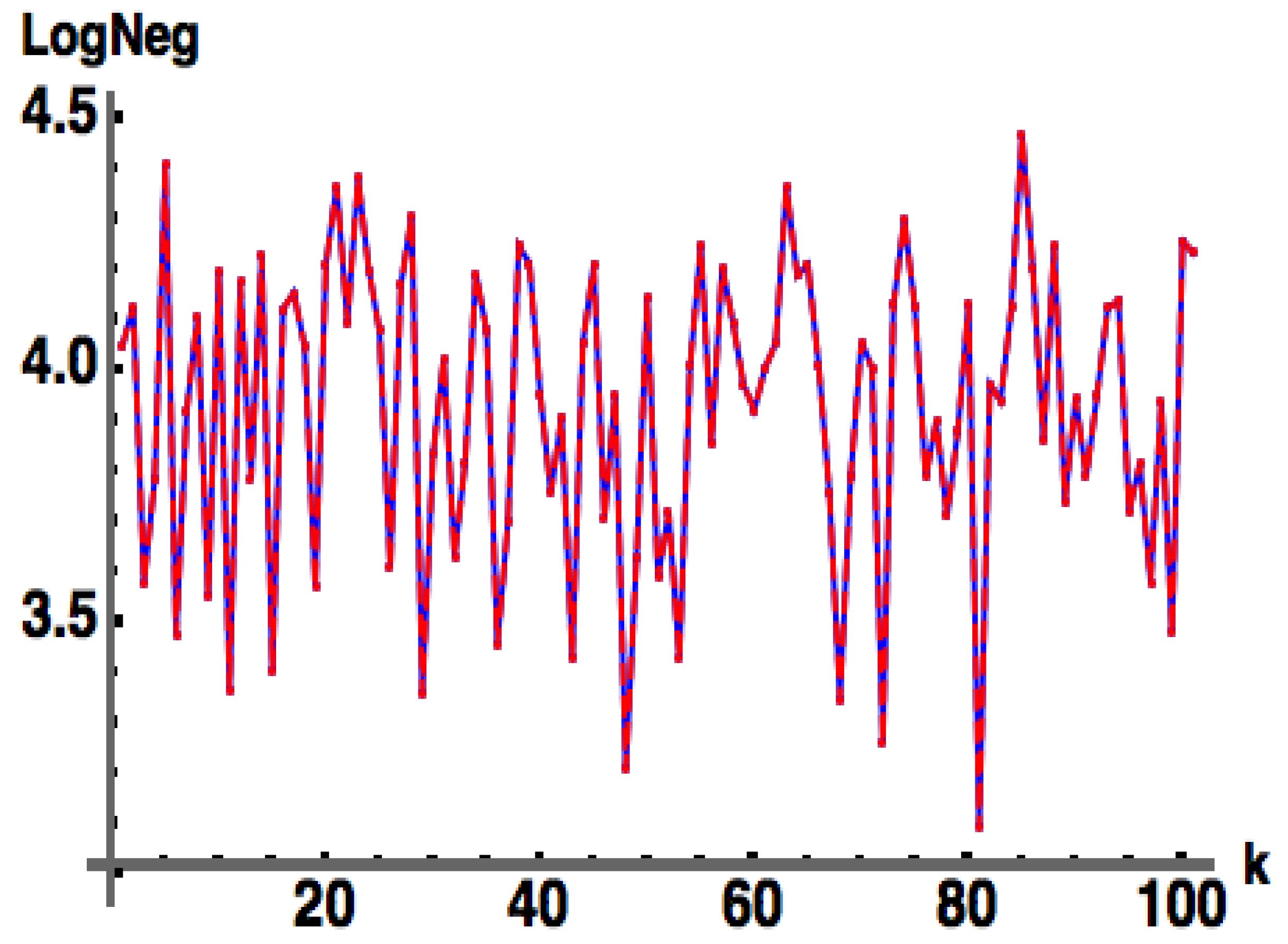
Surprisingly, we have found that Equation (11a,b) produces exactly (obtained from numerically computed eigenvalues) of pure states, for which is a positive Hermitian matrix with both deterministic and random entries as shown in Figure 1. Further, for the case when is a positive Hermitian matrix , we can derive (see Equation (A7a) and Equation (A7b)) the non-trivial result
where the second equalities in the above cannot be derived analytically, but rather are demonstrated numerically from plots such as Figure 1. Here, , which is then flattened (stripped by rows) into an column vector representing . is chosen as a random positive diagonal matrix such that , and U is a uniformly generated (via the Haar measure) random unitary matrix. (Note: is chosen as the absolute value squared of a random row of another randomly chosen unitary .)

Figure 1.
: (blue) exact numerical, (red) approximate from Equation (11b), for pure state with with generated as a positive Hermitian matrix flattened (stripped by rows) into an column vector, with . Here, is a random positive diagonal matrix such that , and U is a uniformly generated (via the Haar measure; see Appendix B) random unitary matrix. (Note: is chosen as the absolute value squared of a random row of another randomly chosen unitary ). In this figure, , with (k) 100 samples as shown. All figures in this work were run with – trials, with only 100 samples illustrated, in order to highlight details (the results were the same regardless of the number of samples chosen).
In Figure 2, we relax the positivity condition on C and change to be chosen simply as a random row of separately generated randomly unitary (vs. the absolute value squared of a random row of for the previous case of ) so that has random complex entries.
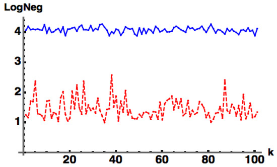
Figure 2.
: (blue) exact numerical, (red) approximate from Equation (11b). This is the same as Figure 1, except now is chosen simply as a random row of separately generated randomly unitary (vs. the absolute value squared of a random row of ) so that it has random complex entries. Here, we take with 100 samples. For any number of samples we always find that , i.e., acts as proper lower bound to .
For any number of samples, we always find that , i.e., acts as a proper lower bound to . This behavior in Figure 2 is the same if we simply take as a matrix of random complex entries. This represents one of the main results of this work. In the following subsection we provide a plausibility argument for Equation (11b) indicating the logic of our “derivation”.
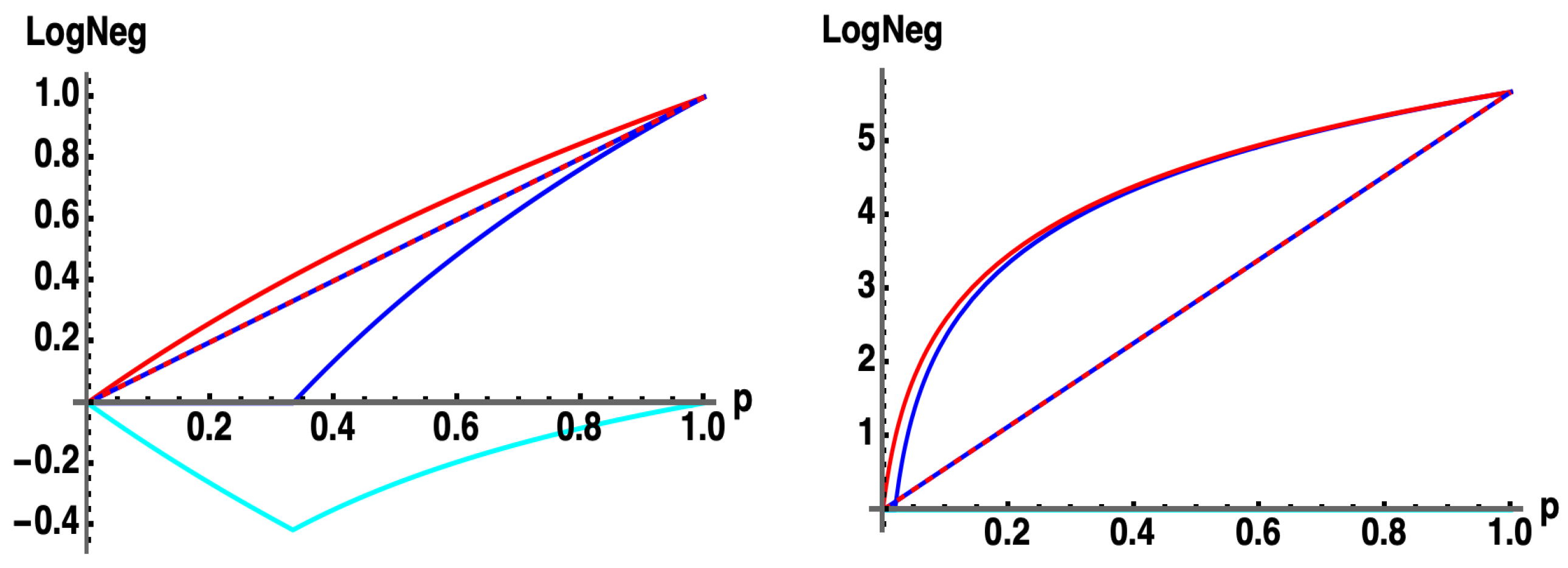
As discussed previously, the use of the Det in Equation (11a) enforces on separable (product) pure states since the Det is identically zero if . This is nicely illustrated for the case of pure states of the form , where . In Figure 3 we show the superposition of two coherent states . The state is separable when where (both exact and approximate).

Figure 3.
: (blue) exact numerical, (red) approximate, for the state . (left) , (right) . The state is separable when where .
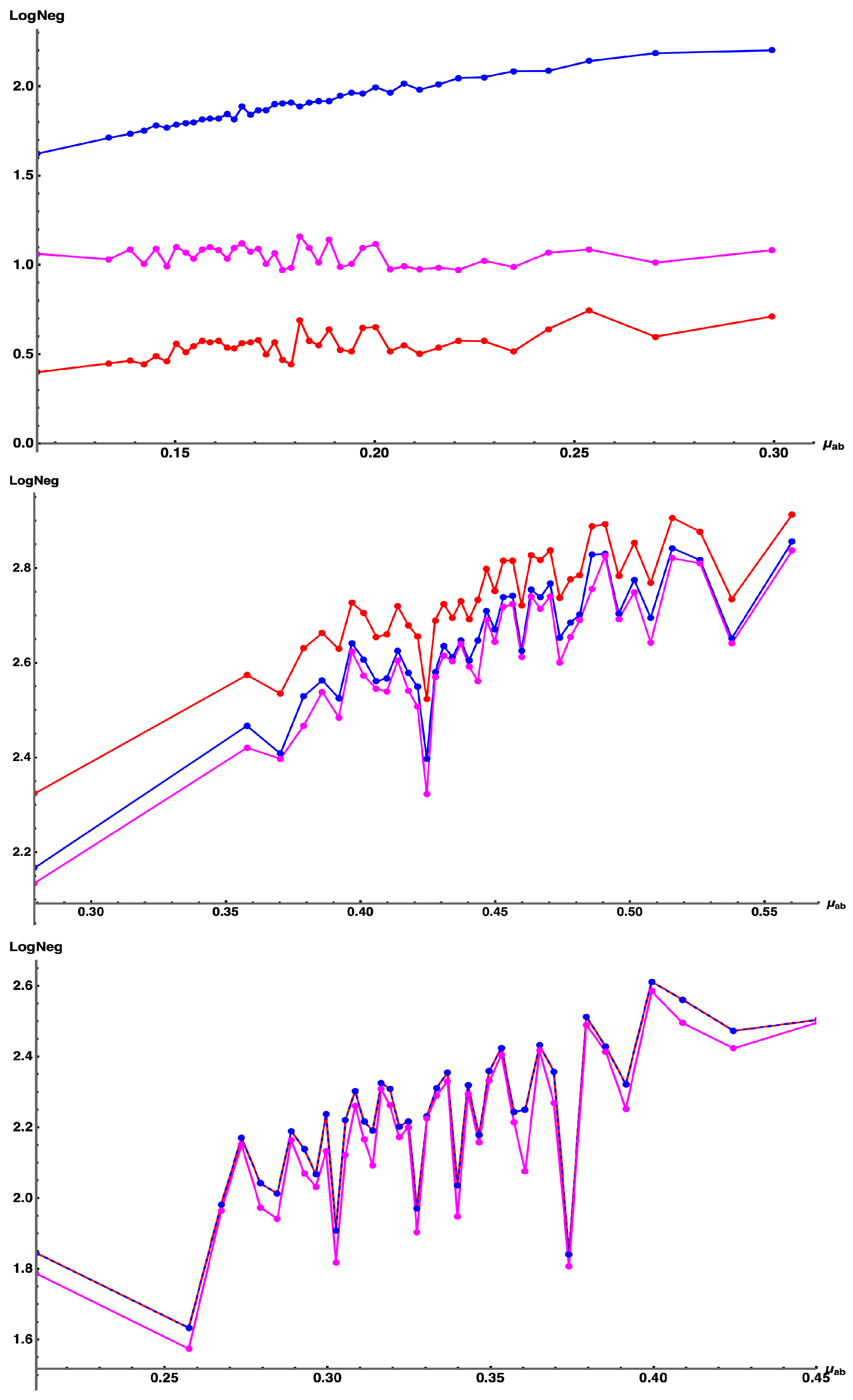
Another way to show that Equation (11b) captures a separable pure state is shown in Figure 4 In the left figure and are taken as two random rows of two different random unitary matrices, while in the right plot, and are taken as two random rows of the same random unitary matrix. In the latter, when the same row is chosen for both and , the state is separable and .

Figure 4.
: (blue) exact numerical, (red) approximate, for the state for with and taken as two random rows of (left) two different random unitary matrices, (right) the same unitary matrix The state is separable when and are the same random vector, where .
3.2. Plausibility Argument for Equation (11a,b)
In this section we present a plausibility argument that led to the “derivation” of the negativity in Equation (11a) and hence the Log Negativity in Equation (11b).
We begin by considering a general pure state . The pure state density matrix is given by . Without loss of generality, and for ease of notation, we treat as real in this subsection, and put in appropriate absolute values at the end of the calculation. Also, we drop the subscript for now. We now write as
The PT is then given by
The first summation in Equation (14a) gives rise to the negativity (putting back in the absolute values) as discussed in Equation (10a) using the eigenstates .
The ansatz we employ is that the negativity is dominated by terms of the form (I), , giving rise to eigenstates , and terms (II), , giving rise to eigenstates , in the PT . We therefore approximate the negativity by only considering “matching terms” of types I and in .
Thus, in the second double summation in Equation (14a), we only consider the terms (i) which give rise to terms of the form .
The first two terms of this expression are diagonal, while the last term gives rise to the negativity as discussed in Equation (10b) using the eigenstates .
However, in the same term in the previous paragraph, we could also consider the case (ii) leading to terms of the form . The last two terms of this expression are diagonal, while the first two again contribute a Negativity of as in the previous paragraph. As part of our ansatz, we conjecture that the terms in Equation (14b) contribute no (significant) terms to the negativity.
Thus, the negativities that we have so far are , which we can write as
where in the last line we have simply used the inequality that with and . As discussed before, using in Equation (15a) overestimates the negativities because the set of eigenstates does not form an orthogonal subset. Thus, we instead use the lower bound given by the determinant expression in Equation (15c). is also the same expression as in Equation (11a), giving rise to the given in Equation (11b).
While the above does not constitute a formal proof or a proper derivation , it is a plausibility argument borne out by numerical evidence. and in Equation (11a,b) also argue that the negativity in a general pure state is dominated by the states and found within , giving rise in the PT to the eigenstates and negativities and , respectively.
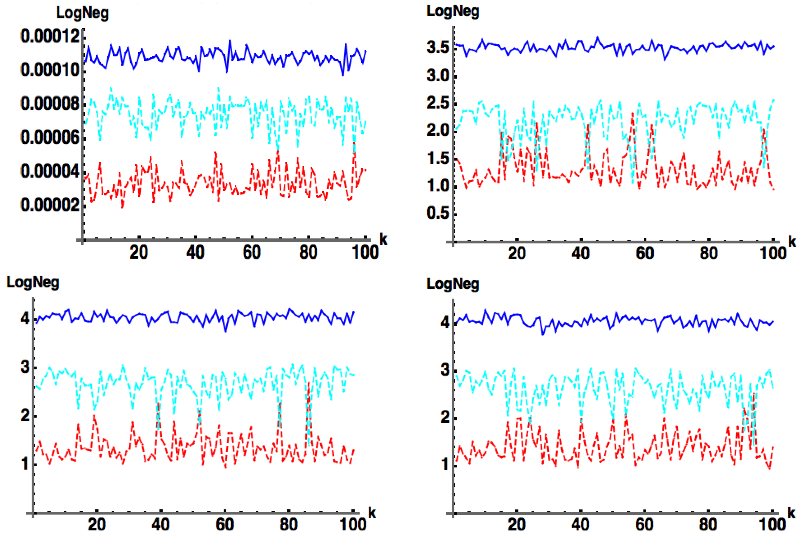
Finally, we return to the case when is separable so that . Let us now consider , where we define , with and Hermitian. If we further define where is an arbitrary d-dimensional complex vector (such that ), then represents an increasing random deviation away from the separable case. In Figure 5 we show plots of , and for , such that , with for increasing values of . We see that acts as a lower bound for . In Figure 6 we show plots of , and for , such that , with for increasing values of . We again see that acts as a lower bound for . Similar behavior occurs for arbitrary values of M.
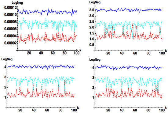
Figure 5.
(blue) , (red) and (cyan) for with for . Here, is an arbitrary d-dimensional complex vector such that and is a random complex matrix, and is an arbitrary real scale factor. (top left) , (top right) , (bottom left) (bottom right) .
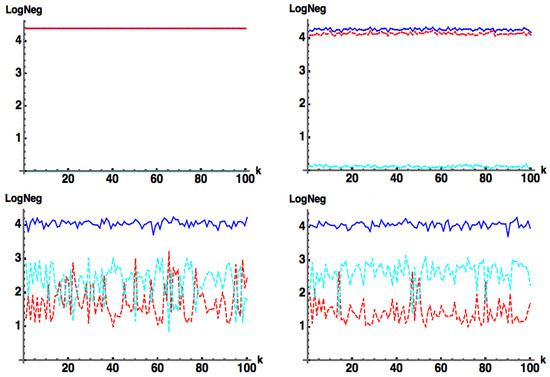
Figure 6.
(blue) , (red) and (cyan) for with for where is the d-dimensional identity matrix such that and is a random complex matrix, and an arbitrary real scale factor. (top left) , (top right) , (bottom left) (bottom right) .
3.3. and for Perturbed Pure States vs. Purity of a Hermitian
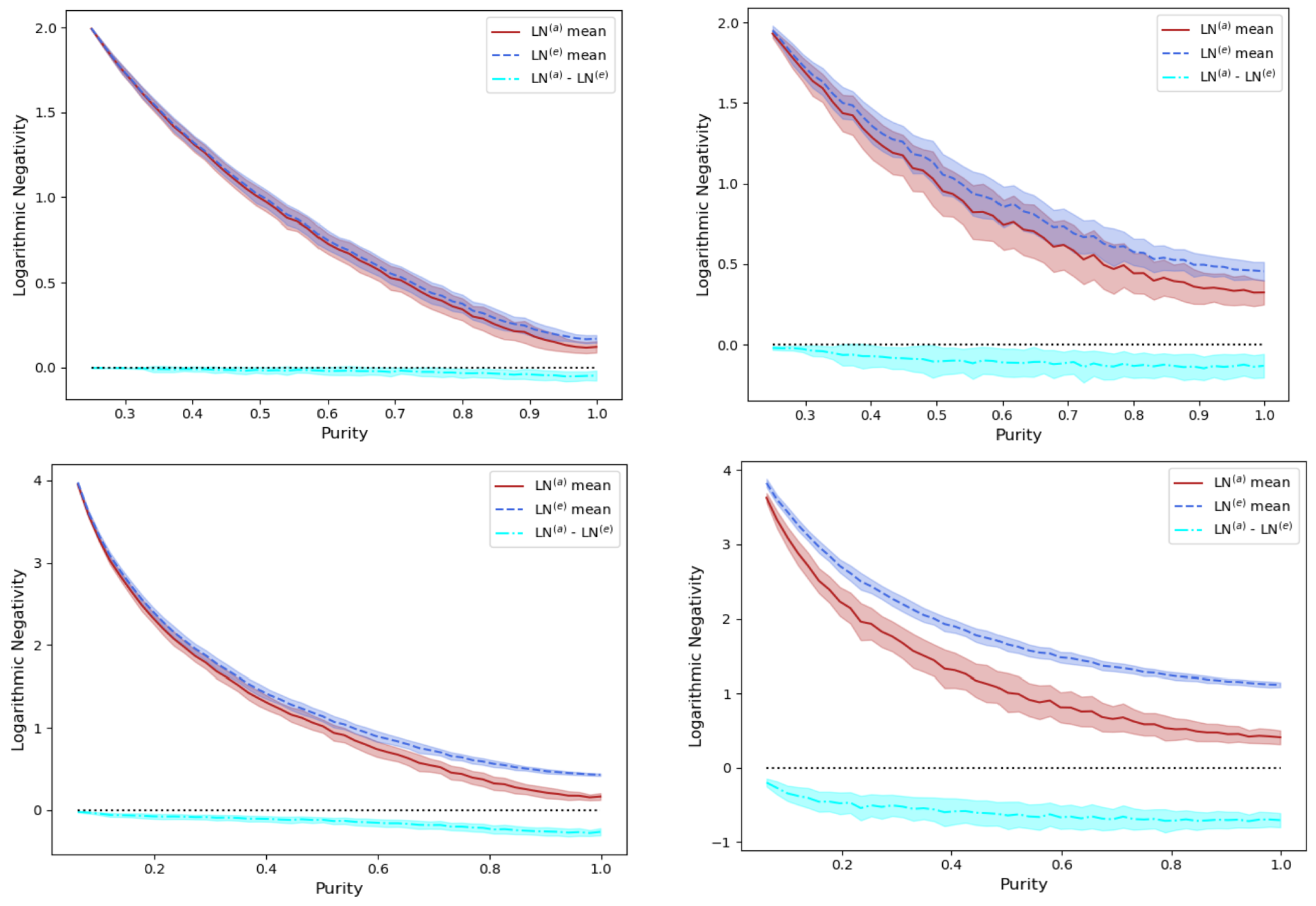
In the previous sections, we examined vs. for pure bipartite states and found that when is considered a uniformly random (with respect to the Haar measure) Hermitian matrix, i.e., C “acts like a density matrix”. We examined this equivalence (random) shot by shot. In this section, we examine the situation when we treat C as a density matrix of fixed purity , for which , but then perturb it away from this result by adding a uniformly random density matrix multiplied by a small “noise” coefficient . In particular we let where . Here is a real, uniformly random, diagonal density matrix of fixed chosen purity value [15] (abscissa), U is a uniformly random unitary, is random Hermitian density matrix, and is a small real parameter. For , C is a Hermitian matrix of fixed purity , and for each uniformly selected C, we have . By allowing , and thus mixing in a uniformly random Hermitian , we perturb C away from its original fixed purity value at . This allows us to sit at a fixed purity and randomly select samples of , and then calculate and compare the mean and standard deviations of and , which are no longer equal for .
In Figure 7 we consider two values of (left and right columns, respectively), for two different values of (top and bottom rows, respectively). The blue-dashed line is the mean of for 100 sample points for each chosen value of the purity . The extreme edges of the shaded blue band about the dashed blue line represent the mean value plus and minus the standard deviation. Similar remarks hold for the solid red line/bands representing , and the solid cyan line/bands representing the difference . From the latter difference cyan curve/band, we see that , namely that even in these statistically perturbed cases (where again, for ), our approximate Log Negativity formula for pure bipartite states where is Hermitian, and acts as a lower bound to .
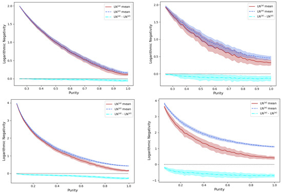
Figure 7.
(blue) , (red) , and difference (cyan) vs. purity for a Hermitian , where (with subsequent normalization ), for a real, uniformly random, diagonal density matrix of fixed purity (abscissa), uniformly random unitary U, random Hermitian density matrix , and real parameter (left,right) , for Hilbert space dimensions (top row,bottom row) . The top and bottom of the colored bands represents the mean plus/minus the standard deviation of each 100 samples of for each value of .
In examining the statistics of Figure 7, note that as in Figure 5 where and the pure d-dimensional state has the highest purity , the bipartite pure state is (counterintuitively) separable, and hence corresponds to , i.e., with minimum value (right side of the abscissa). In addition, as in Figure 6, where , with having the lowest purity , the bipartite pure state corresponds (again, counterintuitively) to the maximally entangled Bell state, and hence to with maximum value (left side of the abscissa).
3.4. Analytic Derivation of for the Bipartite Case of Two Qubits,
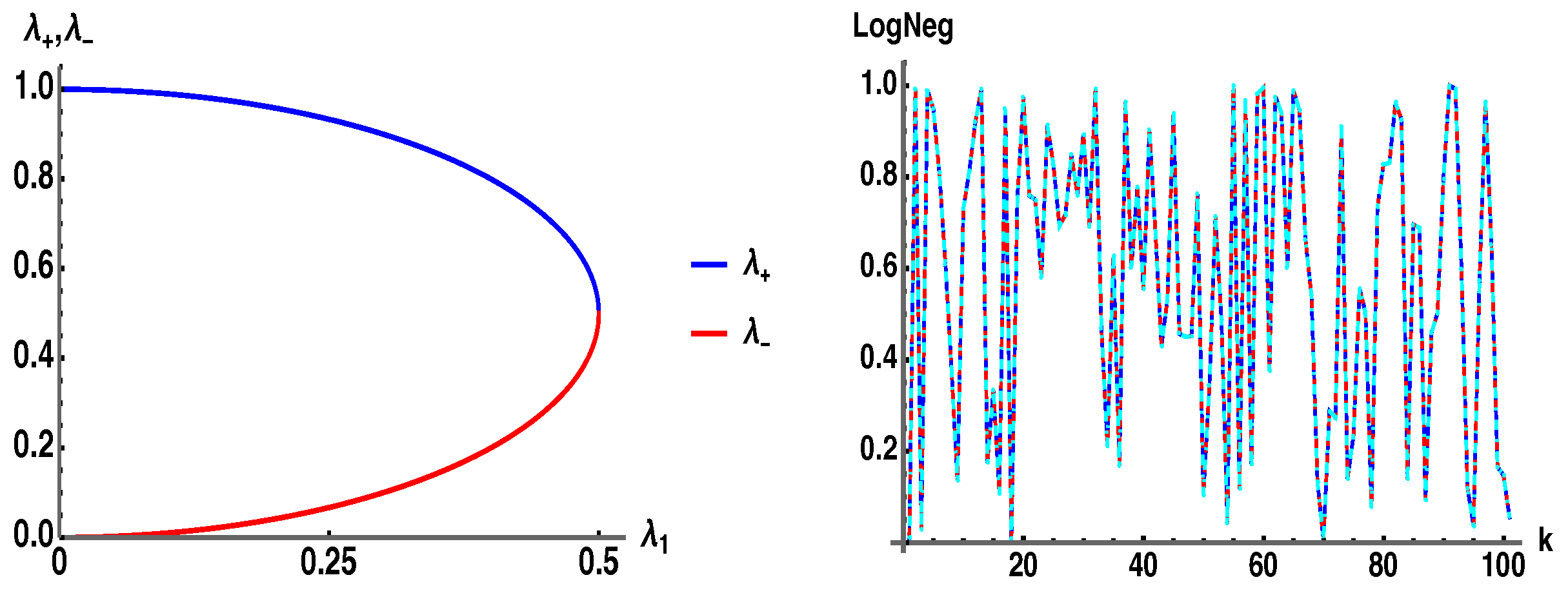
For the case of two qubits (), take to be an arbitrary complex matrix, for which we can analytically obtain the eigenvalues of the partial transpose , Equation (14b), in terms of the . After using the normalization of the state , the eigenvalues of can be written as
Thus, and contributes to the Log Negativity. Since is Hermitian with real eigenvalues, the radical under the square root must be positive , requiring that .
In Figure 8 (left) we plot . In Figure 8 (right) we plot (blue), (red) from Equation (11b), and (cyan) using the analytic eigenvalue in Equation (16b), for the bipartite state of two qubits, . The end result is that for the case of the pure bipartite case of two qubits there is only a single negative eigenvalue of the PT that contributes to the negativity, and it has the precise form of as given in Equation (11a), which has two terms in the sum summing to . For higher dimensions , it is then somewhat unexpected and surprising that in Equation (11a) produces the exact negativity when of dimension d.

Figure 8.
(left) Plot of eigenvalues from Equation (16b). (right) (blue), (red) from Equation (11b), and (cyan) using analytic eigenvalue in Equation (16b) for the case of two qubits, .
3.5. Comparison with Linear Entropy
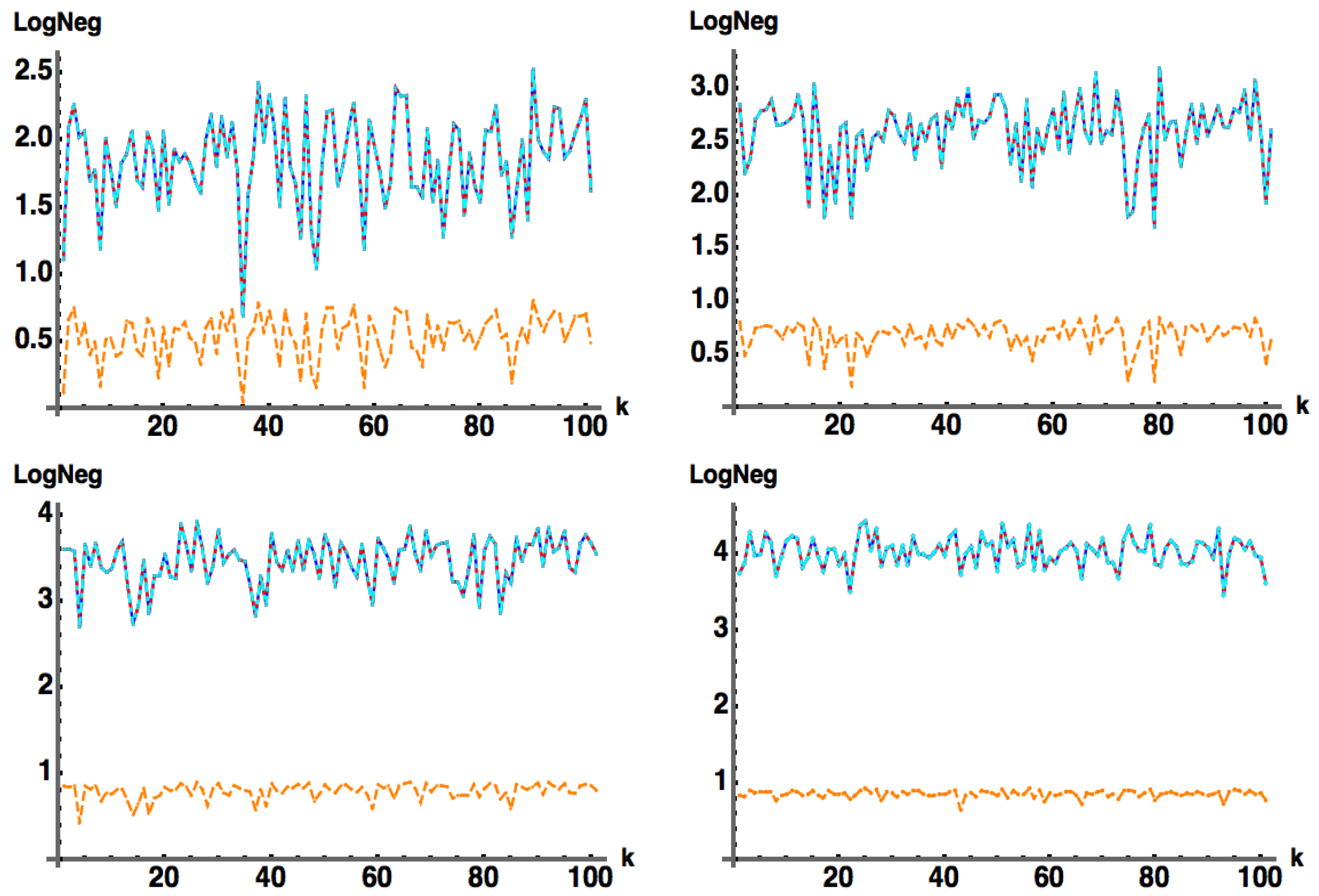
The archetypal measure of entanglement of bipartite pure states that does not involve the computation of eigenvalues is the linear entropy where is the reduced density matrix obtained by tracing out over one of the subsystems. when is separable and when (a matrix) is maximally entangled, and hence (a matrix) is maximally mixed.
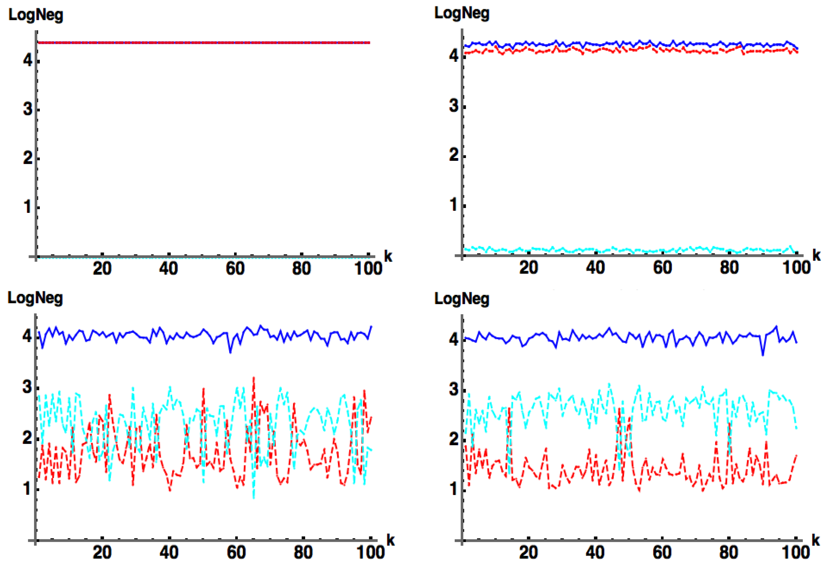
In Figure 9 we plot , , and a variation on the approximate negativity formula Equation (11b) given by (see Equation (A2)), and the linear entropy , when is a positive Hermitian matrix (with ) for . In this case, both and identically equal . The is plotted below (in orange) and acts as a lower bound to .
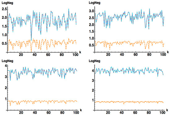
Figure 9.
(blue) , (red) , (cyan) , and (orange) when is a positive Hermitian matrix (with ): (top left) , (top right) , (bottom left) (bottom right) . Note, the blue, red, and cyan curves overlap exactly in all these figures.
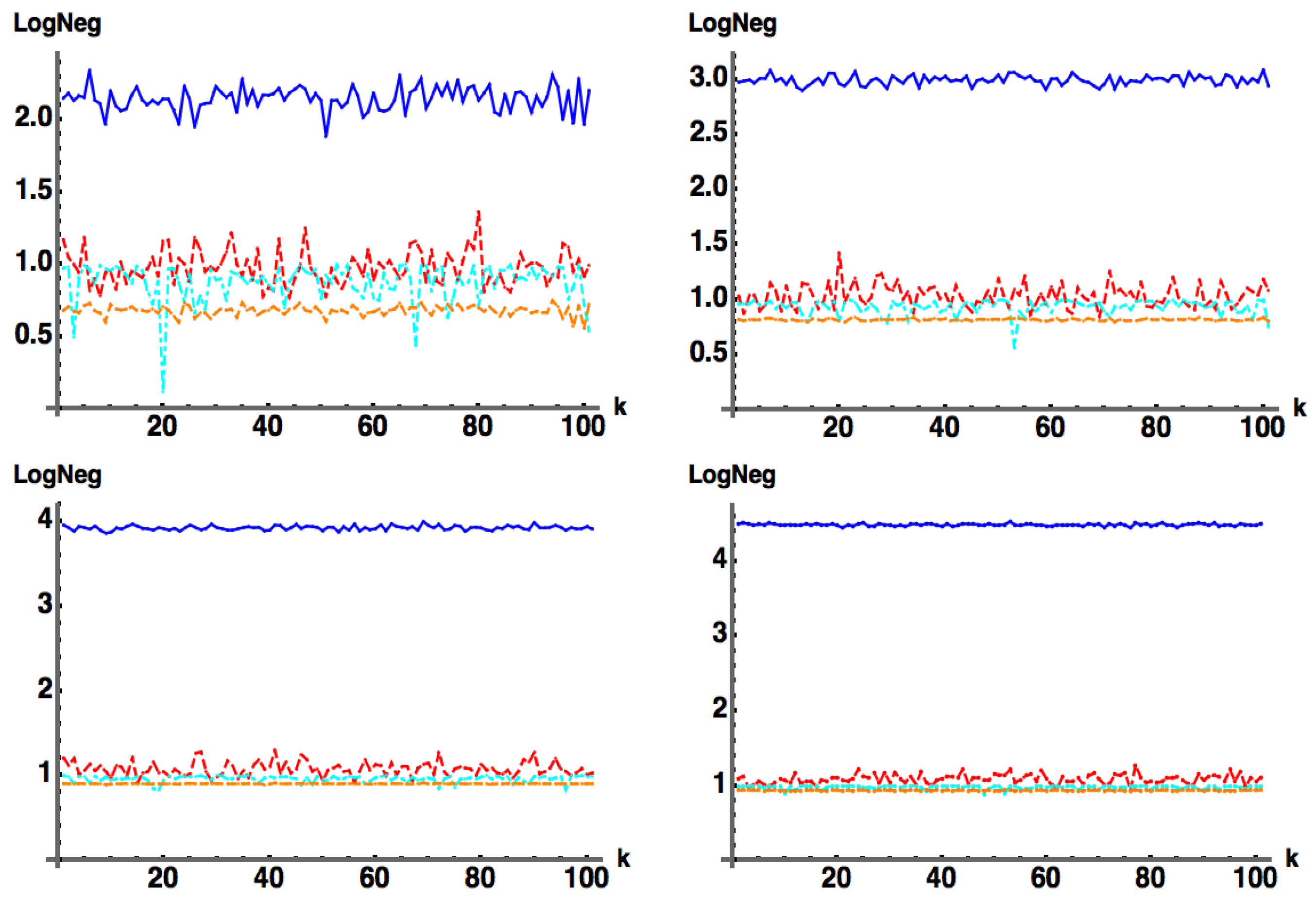
Figure 10 is identical to Figure 9, except we now allow to be a random complex matrix. We see that acts as a better lower bound than , which is in turn a better lower bound than the . As the dimension d increases, the latter three measures are observed to converge to approximately the same lower bound values, with still performing as a slightly better lower bound.
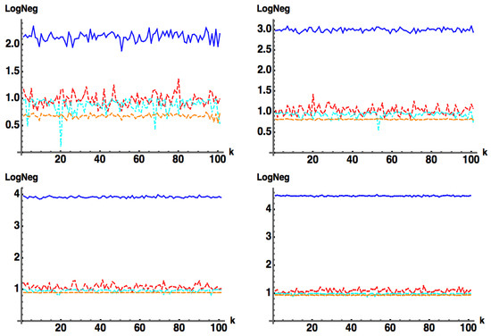
Figure 10.
(blue) , (red) , (cyan) , and (orange) when is a random complex matrix (with ): (top left) , (top right) , (bottom left) (bottom right) . (Compare with Figure 9.)
4. An Attempt to Extend to General Density Matrices
Extending the negativity and Log Negativity from Equation (11a,b) appropriate for pure states to mixed states is a non-trivial task. In principle the extension of an entanglement measure to mixed states is easy to state but computationally involved to perform [16]. Given a pure state (ensemble) decomposition (PSD) of a mixed state and an entanglement measure E on pure states, one can form the average entanglement . The entanglement measure on mixed states is then taken as the minimum of over all possible PSDs (the so-called convex roof construction). This final result is sometimes referred to as the entanglement of formation, which quantifies the resource required to create a given entangled state. Since is a convex function, one can apply Legendre transformations [17] to transform the above difficult minimization into the “minmax” problem [18] , where the exterior maximum is taken over all Hermitian matrices X. The dimension of the exterior optimization over X can be reduced to a rather small number by the symmetry of the state , which greatly simplifies the numerical task as was demonstrated in [19].
In this work we are not interested in forming a proper entanglement measure, rather a witness, that can lower bound the exact Log Negativity. Therefore, we will forgo the above computationally involved procedure and instead put forth (while somewhat simplistic but computationally tractable) an ansatz for a straightforward generalization of our pure state witness.
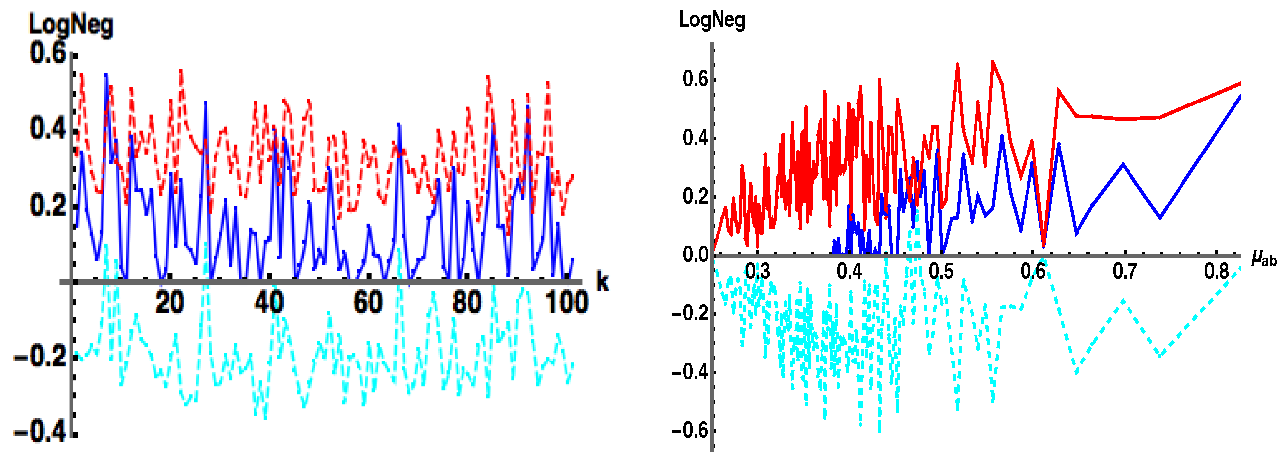
The main advantage of Equation (17b) is that upon reduction to a pure state , the above formulas reduce to Equation (11a,b). However, as Figure 11 shows, Equation (17b,c) now acts more as an approximate upper bound as the dimension d increases (left), versus a desired lower bound, but typically at higher purity values (right). Note that does a fairly good job of tracking the up and down random fluctuations of but the former does not do a very good job when the latter is zero. On the negative side, Equation (17b) does not capture separability when . The issue of witnessing separability in general is a difficult, non-trivial problem [12], so it is not surprising that a simple generalization from a pure state witness to a mixed state witness would not be valid. Nonetheless, Figure 11 is intriguing for the relative tracking of with . acts “almost” as an upper bound to , (i.e., the cyan difference curve ), but there are places where it also acts as a lower bound, i.e., .
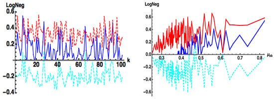
Figure 11.
: (blue) exact numerical, (red) from Equation (17c) (cyan) , for random with (left) , (right) (two qubits).
4.1. on Werner states
Because they are analytically tractable, it is informative to examine the proposed mixed-state witness Equation (17c) for the case of Werner states of dimension (where ), i.e.,
(Note: is a vector, so is a matrix). In Figure 12 we show and for Werner states with (top) (two qubits) and (bottom) using the approximation for the negativity given in Equation (17c).
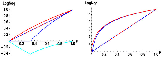
Figure 12.
: for -dimensional Werner states with probability (to be in the pure state) : (blue, solid) , (red, solid) from Equation (17c), (cyan) . Average Log Legativity (ALN) (blue, dashed) , (red, dashed) , for uniformly random with (left) , (right) . Note: throughout all of . (overlapping red-dashed and blue-dashed curves).
Here we also introduce the Average Log Negativity (ALN) (for both exact and approximate ) given by for mixed states of the form . It is straightforward to compute that for the Werner state, the negative eigenvalues of the partial transpose are given by
Therefore, the negativity in this region is given by
yielding
Thus, is entangled () for , and separable () for . Finally, one can also show that the purity for the Werner states is given by . This corresponds to a critical value , equivalently , where the value of the Log Negativity drops to zero. Some authors [16] refer to phenomena as the “sudden death of entanglement” since in the region , is separable, while is entangled for .
On the other hand, for a given , for Werner states, we have
yielding again
vs. at as for . Therefore, (red curve) never detects separability, and for Werner states, acts as a strict upper bound for (blue curve). Further, for Werner states as demonstrated in the bottom plot in Figure 12 with . Note that in the limiting case of , the Werner state is always entangled, and never has a region of separability.
The sudden death of entanglement at introduces a derivative discontinuity in that arises from the definition that the negativity is defined as non-zero only if some eigenvalues of the partial transpose of the density matrix are negative. Equivalently, such a discontinuity could also be introduced for the Werner states by declaring that iff . Our definition of the continuous function can never capture this derivative discontinuity. For Werner states one could attempt to capture this feature for any definition of a by simply defining for .
A symmetrization of Equation (17b) is given by
which also reduces to Equation (11a,b) for the case of pure states . (Note that one could also add terms such as which reduce to zero on the pure state case . However, we have not found such additional terms useful). Equation (24) also has the additional favorable property that it does detect separability iff, for each i, either or are zero. This occurs because if , Equation (24) reduces to
where the terms inside the absolute value are proportional to the product of . This implies that either term in the product needs to be zero as a necessary and sufficient condition for the approximate negativity in Equation (19) to yield zero on separable states.
Equation (24) does detect a wide class of separable states, but of course, not all. This is especially apparent since the application of Equation (24) to the produces exactly the same plots as shown in Figure 12. We can understand this as follows. For the case of two qubits (), we can write
While Equation (26a) is valid for all values of , Equation (26b,c) is only valid mixed-state representations (since each of the four terms is diagonal in a separable basis, and positive semi-definite) provided that . Now the term involves density matrices and that are both complex, for which our witness in Equation (24) cannot detect separability since at least one of the or would need to be real .
4.2. Average as a Lower Bound for
We note that for Werner states, the Average Log Negativity (ALN) for both the exact , and the approximate version (using Equation (17c) on the right-hand side), are identically equal throughout all of , even in the separable region where , as shown as the overlapping dashed blue and red lines in Figure 13. This is because on the components of the pure symmetric Bell state density matrix, and also on the maximally mixed state (yielding value on the latter). In fact, we see that the is concave in the region where entanglement is present, and is convex in the region where the state is separable. On the other hand, our is concave throughout all of . Thus, as the dimension increases, becomes an increasingly better lower bound for for a larger region of p as the region of separability decreases as shown in Figure 13 for , and for in (bottom) Figure 12.
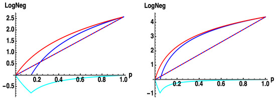
Figure 13.
: for -dimensional Werner states with probability (to be in the pure state) : (blue, solid) , (red, solid) from Equation (17c), (cyan) , Average Log Negativity (ALN) (blue, dashed) , (red, dashed) , for uniformly random with (left) , (right) . Note: throughout all of . (overlapping red-dashed and blue-dashed curves).
The above properties on Werner states prompt us to compare to for more general random density matrices written as a pure state ensemble decomposition (PSD), , which we consider (only) for the remainder of this section. We also introduce an additional version of the average approximate Log Negativity given by
which now uses our approximation of the Log Negativity for pure states via Equation (11b) on the ensemble pure state components on the right-hand side, which is denoted as . This is to be distinguished from the notation , which we will reserve to denote the Log Negativity using our approximate mixed-state formula Equation (17c), and which is the average approximate Log Negativity that also uses Equation (17c) on general mixed states .
The trend seen in the above Werner state discussion appears to hold in general for PSDs, namely that as the dimension of the pure state components increases, becomes an increasingly better proper lower bound of as shown in Figure 14 (top).
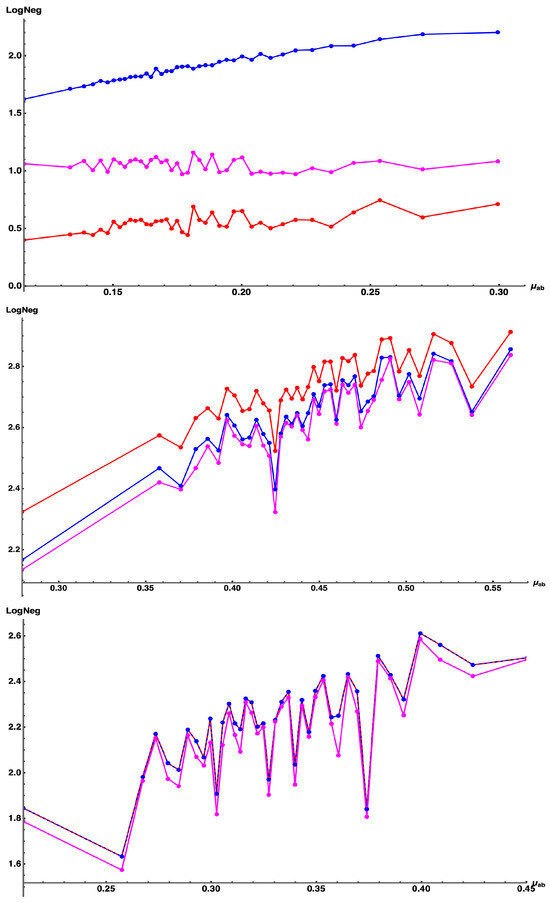
Figure 14.
and vs. for PSDs with , and , plotted against purity . Each is chosen as (top) a random complex matrix, , (middle) random Hermitian matrix , (bottom) random Orthogonal matrix . Color legends: (blue) , (magenta) , (red) . The blue and red curves overlap in the bottom figure, .
Here and is given by the blue curve, by the red curve, and by the magenta curve. We are interested in the comparison of the red and magenta curves to the blue curve, based on how the matrices are chosen in each pure state component of the PSD, where , with . In Figure 14 (top), the are chosen as a random complex matrices. For this case we have (red, magenta, blue curves) as the dimension increases. For Figure 14 (middle), the are chosen as random Hermitian matrices. Here there is a dramatic change in structure. For this case we have (magenta, blue, red curves), for which has switched to a proper upper bound of , and these inequalities hold all the way down to , the case of two qubits. Further, both and track the fluctuations of surprisingly, extremely well. Finally, in Figure 14 (bottom) the are chosen as random orthogonal matrices, and now, very surprisingly, we find that we have (magenta, blue overlapping red curves), namely that becomes exactly equal to , while remains a lower bound (which appears somewhat tighter than in the previous Hermitian case). Again, these inequalities hold all the way down to , the case of two qubits.
In general we have found that for written as a PSD, based on our pure state negativity approximation given in Equation (11b) does a better job of acting as a lower bound to than based on the mixed-state negativity approximation given in Equation (17c). As discussed in the Introduction, Equation (2), and shown in Figure 14, we have numerically found that
when the mixed state is written as a pure state decomposition (PSD) , and in addition, the quantum amplitude matrix of each pure state component is uniformly generated (over the Haar measure) as a positive Hermitian matrix, . Further, we find that the second inequality is surprisingly saturated, i.e., in Equation (28), if the uniformly randomly generated matrices above are real, i.e., . A discussion of the uniform generation of Hermitian matrices over the Haar measure used in these numerical studies is given in Appendix B.
5. Other Approaches to Bipartite Pure-State Entanglement Quantities Without Matrix Diagonalization
A proper measure of entanglement for bipartite pure states is the von Neumann entropy (VNE) given by , where are the eigenvalues of the reduced density matrix , necessitating the need for the diagonalization of . There has been much theoretical and experimental interest in methods for direct detection of the VNE or other quantifiers of entanglement that do not require diagonalization [20,21,22,23,24,25,26]. In the paper by Meurice [26], concerning configurable arrays of Rydberg atoms, they were able to obtain robust and reliable estimates of the VNE using bitstring mutual information from measurements. In the computational basis , the estimated VNE is , where the superscript X is short for eXperimental. In this basis, the diagonal elements are the probabilities for bitstring (projective) measurements. Forming the marginal distribution , the reduced experimental entropy , and the experimental mutual information , they found the upper and lower bound for the exact VNE given by .
5.1. Rényi, Tsallis and Linear Entropy
The necessity of the diagonalization of obviously stems from the use of the non-linear function in the VNE. For Taylor expanding about , we have , from which we can write the VNE as
where we have used the binomial expansion for , and written . Equation (30) reveals that formally one could dispense with the necessity of diagonalizing the reduced density matrix in place of knowing all its moments for . The most widely used approximation of the VNE used in the literature is the term in Equation (29), namely, the linear entropy ,
which is why it is often claimed that the LE is “qualitatively equivalent” to the VNE, although recent work has shown that the former can dramatically disagree with the latter, for example, in low-density regimes of fermionic systems [27]. Note that if we tried to obtain a “better approximation” by retaining just the and terms in Equation (30), we would obtain , which diverges (i.e., we cannot switch the order of the summations). Thus, the term is the linear approximation to the VNE, and has been widely used in the literature, characterizing entanglement in a variety of systems, without the need to diagonalize (see references [22–43] of [27]).
The LE is the case of the Quantum Tsallis q-entropy defined as
which is related to the Rényi entropy
by
Both the Rényi and the Tsallis entropies converge to the VNE in the limit .
The LE has many positive analytic properties such as subadditivity, pseudo-additive for product states, and a lower bound (Araki–Lieb inequality from subadditivity) [28]
In Section 3.5, we compared our approximate Log Negativity for pure bipartite states to the LE and found that in our numerical experiments, was typically greater than the (while both being less than the exact Log Negativity ), and thus formed a better lower bound to .
5.2. The Special Case of 2-Qubits, Concurrence and Linear Entropy
In Section 3.4 we examined the case of 2-qubits () and found that our approximate Log Negativity was analytically equal to the exact Log Negativity since the negativity was given by (the absolute value of the negative eigenvalue of the partial transpose , namely) , Equation (16a). For the special case of a 2-qubit pure state, is in fact the Wootter’s concurrence [10,21,29,30]
where is the local spin-flip operator acting on both qubits individually, taking each qubit to the orthogonal state diametrically opposite on the Bloch sphere, along with a conjugation operation. In addition, is also the exact value of the LE when normalized (as is often found in the literature) as .
Attempts have been made to generalize concurrence to arbitrary dimensions by generalizing to a general for an arbitrary system [30,31], and by superoperator methods [32]. For any conjugation , one can define the -concurrence of a pure bipartite state as (and for a mixed state as for an ensemble decomposition ).
For a pure state bipartite system with with labeling two specific basis states for subsystem a, and with labeling two specific basis states for subsystem b, let be an ordered set of two pairs of labels. Following [31], Wootters [30] considers the higher-dimensional antilinear conjugation operation for a given ordered set defined by
As Wootters states [30], projects an arbitrary state of the system onto a “two-qubit subspace” and then performs what amounts to a spin-flip on that subspace. For each , collect the into a concurrence vector. Wootters shows that the length of the concurrence vector is invariant under local unitary transformations of the two separate subsystems and is given by
where the latter result agrees with that of [32] using the superoperator formulation where . Wootters’ method of projection onto two-qubit subspaces is very much in the spirit (but different in implementation since Equation (39) reproduces the LE) of what our approximate Log Negativity formula is doing in Equation (11a,b) i.e., treating in as a collection of two-qubit “subspace”, labeled by indices , but where n and m are taken only on the diagonal of . The relationship between our work and Wootters’ concurrence vector will be explored in future work.
6. Summary and Conclusions
In this work we presented numerical evidence for a witness for bipartite entanglement based solely on the coefficients of the pure state wavefunction as opposed to the eigenvalues of the partial transpose of , as appropriate for the Log Negativity. This is achieved by approximating the negativity by diagonally dominant determinants of the coefficients as given in Equation (11a). This agrees exactly with the exact negativity (given by the standard definition obtained by the sum of the absolute values of the negative eigenvalues of the partial transpose ) when is a positive Hermitian matrix (i.e., C is itself a non-unit trace density matrix). Interestingly, these include the cases when (i) C is considered a maximally mixed density matrix, then is the maximally entangled d-dimensional Bell state, while (ii) if C is a pure state density matrix, then is separable, and (iii) symmetric superpositions of pure states with real coefficients. In these cases, . Of particular relevance is that for C being a general complex matrix, we find that acts as proper (but not tight) lower bound for , i.e., .
In the second half of this work, we attempted to generalize our approximation of the negativity from pure states to mixed states via Equation (17b), which reduces to the diagonally dominant determinants formula Equation (11a) for pure states. We met with partial, yet still interesting, success. One of the key features of a negativity based on Equation (24), a symmetrized version of Equation (11a), is that it yields on separable states when either one of the component separable states or is , real. While this of course does not capture all separable states (a non-trivial task), it does capture a wide range of physically relevant density matrices.
In general, we found that a based on Equation (24) acts more as an (undesired) upper bound to as demonstrated vividly on the analytically tractable d-dimensional Werner states. However, for Werner states we saw that as the dimension d grew large, and the corresponding region of separability grew smaller as .
This led us to consider for pure state ensemble decomposition (PSD) of the density matrices , now using our approximation of the pure state negativity via Equation (11a). Again, we saw that as the dimension d of the pure state components increased, acted as a proper lower bound to , i.e., . We speculate that this occurs for similar reasons to for the Werner states, namely that as the dimension d increases, the region of separable states becomes vanishingly small [9,33], and simultaneously our negativity formula Equation (11a) is more accurate on pure states than Equation (17b) on mixed states, and hence the former does a better job of acting as a lower bound.
In summary, the main features of our proposed entanglement witness are (i) a simple formula for an approximate negativity Equation (11a) on bipartite pure states directly in terms of the quantum amplitudes of the quantum states that is also exact for a certain class of physical relevant states (with the Log Negativity related to the negative log of the purity of the quantum amplitude (matrix) when they have the properties of a normalized density matrix, Equation (12c)), and (ii) this negativity formula does not require the need to numerically compute eigenvalues of the partial transpose of the density matrix. An attempted generalization of this pure state negativity formula for pure states to mixed states yields that (iii) in simulations on pure state decompositions (PSDs) of density matrices where the quantum amplitudes of each of the pure state components act as positive Hermitian matrices, Equation (27), based on the Log Negativity approximation for pure states Equation (11b), yields a proper lower bound to , and (iv) on the PSD of density matrices in (iii), provides a proper upper bound to (with equality when are orthogonal matrices), and most interestingly, both and track, extremely well, the fluctuations in for uniformly randomly generated states.
As stated in the introduction, the numerical computation of eigenvalues does not present a practical impediment to the calculation of entanglement measures. Rather, it is the surprising and unexpected relationship (and equality for certain physically relevant states, both pure and mixed) between the entanglement witness we propose and the exact Log Negativity that was the impetus for this current investigation. In essence, the main contribution of this work is an extension of the class of states that are amenable to Agarwal’s [13] method of exact analytical diagonalization. Our conjecture is that these two types of exactly analytical diagonalizable states form the dominant contribution to the entangle of the state as measured by our approximate Log Negativity formula. What is unexpected and surprising is that (i) it yields exact results on a limited class of pure state, (ii) acts as a lower bound (what we refer to as an entanglement witness) on arbitrary pure states, and, even more surprisingly, (iii) yields exact results on a limited class of mixed states. It is our hope that this work might inspire further investigations into a more complete foundational (and proper) derivation underpinning the results presented in these numerical investigations.
Author Contributions
Conceptualization, P.M.A.; Software, R.J.B.; Formal analysis, P.M.A.; Investigation, R.J.B.; Writing—original draft, P.M.A.; Writing—review & editing, R.J.B. All authors have read and agreed to the published version of the manuscript.
Funding
This research received no external funding.
Institutional Review Board Statement
Not applicable.
Informed Consent Statement
Not applicable.
Data Availability Statement
The original contributions presented in this study are included in the article. Further inquiries can be directed to the corresponding author.
Acknowledgments
Any opinions, findings and conclusions or recommendations expressed in this material are those of the author(s) and do not necessarily reflect the views of their home institutions. The authors would like to thank J. Schneeloch and C.C. Tison for numerical code support for the figures in Section 3.3.
Conflicts of Interest
Author Richard J. Birrittella was employed by the company Booz Allen Hamilton. The remaining authors declare that the research was conducted in the absence of any commercial or financial relationships that could be construed as a potential conflict of interest.
Appendix A. Proof of Equation (12a)
From Equation (11a) let us define as the lower bound to the approximate Negativity by
Now
Recall that with is a complex matrix subject only to the constraint . Thus let us define another arbitrary complex matrix A via
noting that is a positive matrix. Thus Equation (A2) becomes
Now let us impose some additional conditions on A and hence C.
- Case 1: is Hermitian.
- Case 2: is Hermitian and . Note that does not imply that A is positive since A could have negative real values on the diagonal such that .
- Case 3: is Hermitian, positive and , i.e., is an un-normalized density matrix. Then
It is in this latter Case 3 that we find numerically that . Equation (A7a) is Equation (12a).
Lastly, we consider the following case.
- Case 4: is Hermitian, positive and , i.e., is a proper density matrix itself. Then
Appendix B. Random Unitary Matrices, and Sampling of Density Matrices over Purity Ranges
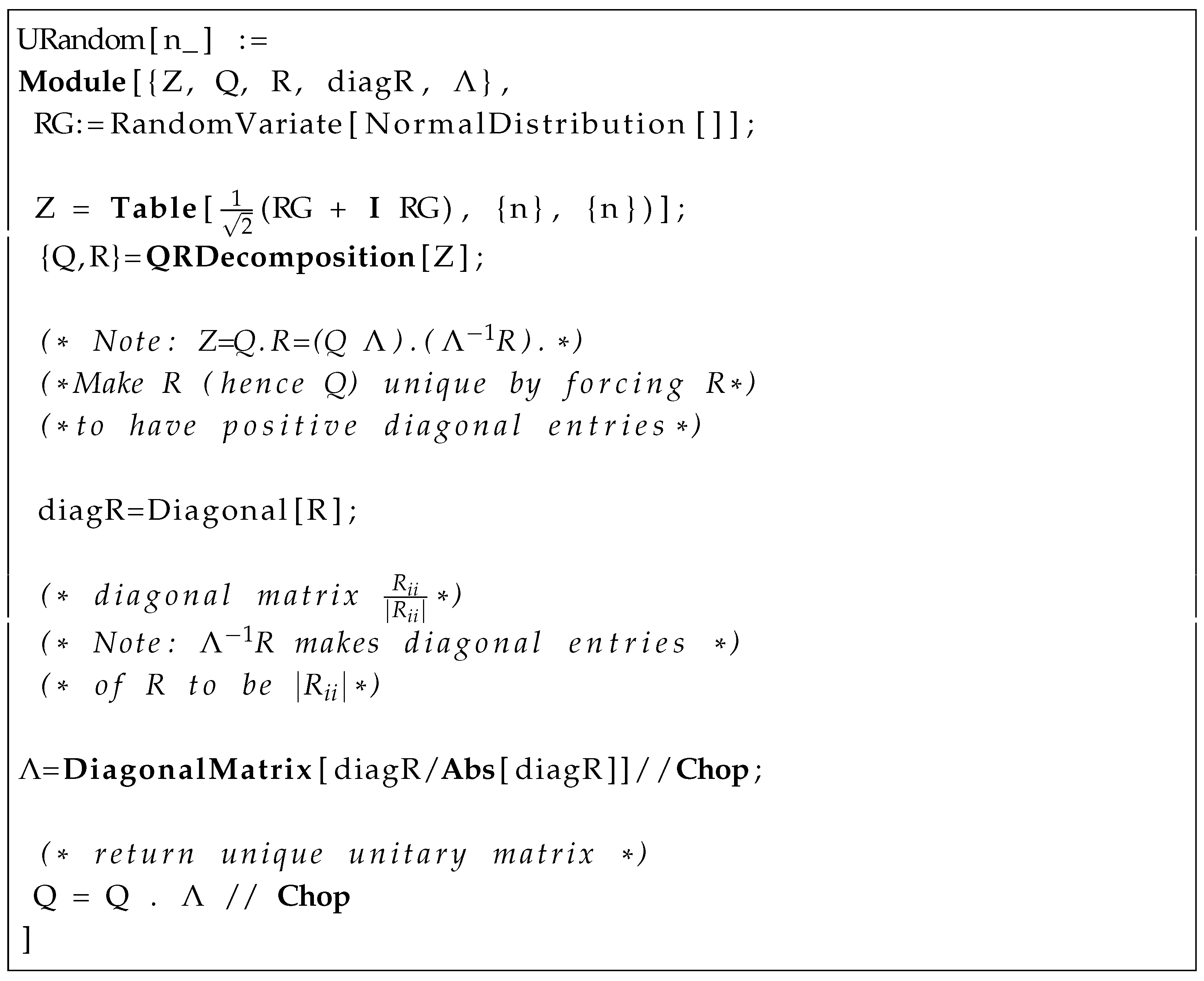
| Listing 1. Mathematica code to generate random unitary U. |
 |
| Listing 2. Mathematica code to generate random ρ. |
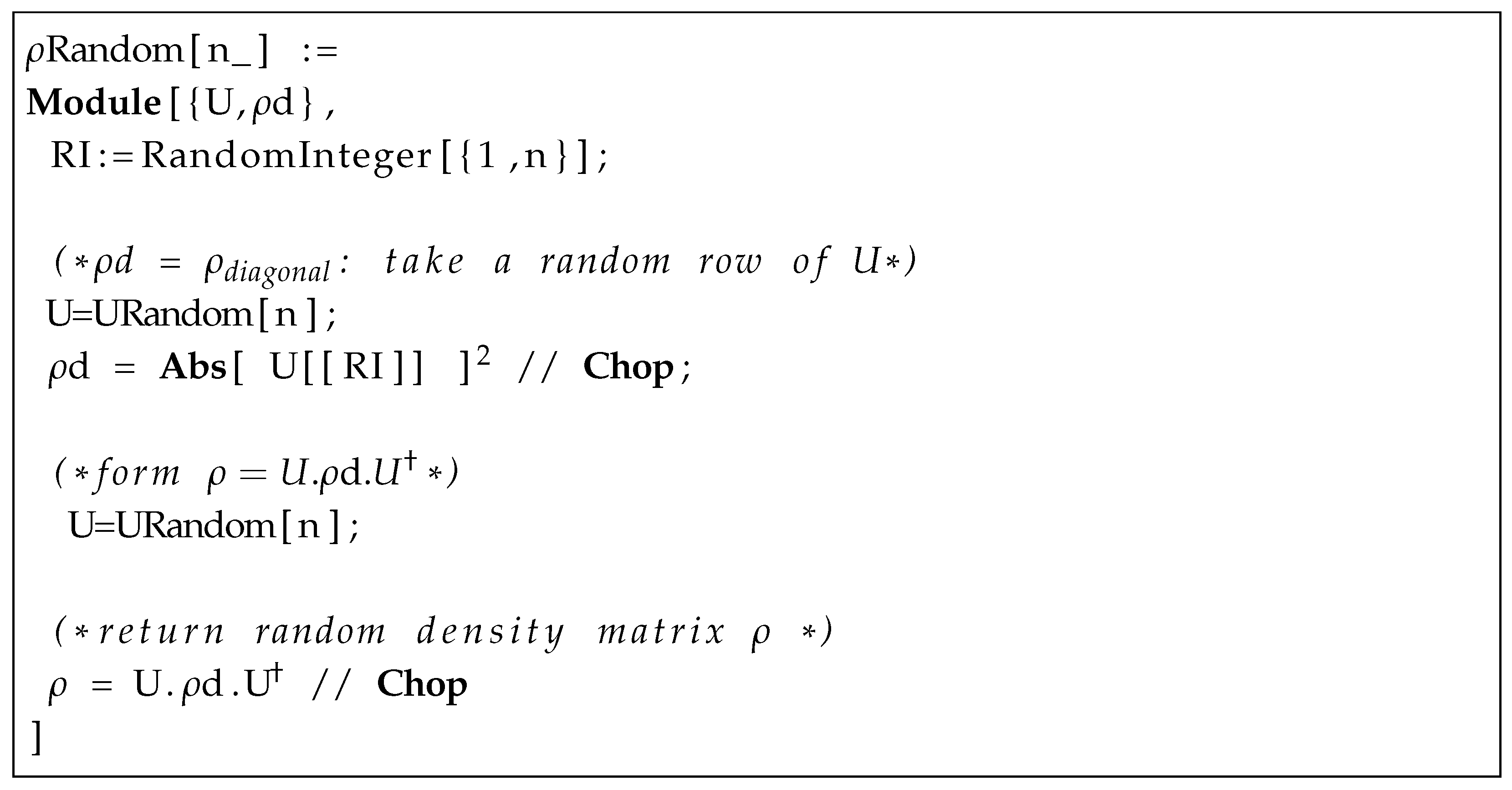 |
The above are the Mathematica codes used to generate uniformly random unitary (and orthogonal) matrices (via the Haar measure), and subsequently uniformly random density matrices, based on the article by Mezzadri [34]. The central idea behind these codes is that the space of invertible complex matrices (the Ginibre ensemble) have matrix elements that are independent identically distributed (i.i.d.) standard normal complex random variables with probability distribution . The joint probability distribution for the matrix elements (also statistically independent) is given by . is normalized to unity via where and . The integration measure on the Ginibre ensemble is which can be thought of as an infinitesimal volume in . The crucial point is that is invariant under left and right multiplications of Z by arbitrary unitary matrices i.e., for . The proof follows trivially from the property of the trace in the definition of since , and hence . This Haar measure is the matrix analogue of a uniform probability distribution in one dimension .
The above algorithm to generate random unitary matrices distributed with the Haar measure uses the decomposition of Z (vs. the less stable, at higher dimensions, Gram–Schmidt orthonormalization routine). Here Q is a unitary matrix and R is an upper-triangular matrix. However, one caveat exists. The decomposition is not unique, since if then so is , with as a diagonal matrix such that and are again unitary and upper-triangular matrices. To make the decomposition unique, the solution (see Mezzadri [34] for details) is to choose where are the diagonal elements of R. Thus, the diagonal matrix elements of are real and strictly positive, which renders the matrix unique and uniformly distributed with the Haar measure. This is the procedure implemented in the above Mathematica codes.
Given a code to generate random unitary matrices U, one can subsequently generate uniform density matrices (positive Hermitian matrices of unit trace) by the simple decomposition . To generate the diagonal density matrix (an element of the Weyl chamber, Section 8.5 of [9]) such that , one simply generates another random unitary and takes the absolute square of the random row (or column) as the the diagonal entries. This is implemented in the second code listed above. These codes are easily implementable in other commonly used coding languages, such as Python.
While the codes above generate uniformly (Haar) distributed density matrices , the purity of such generated matrices are distributed non-linearly. This is because the Haar measure enforces linear constraint on the eigenvalues of , the purity is given by the non-linear (quadratic) constraint . In general, a Haar distributed tends to sigmoid shaped distribution in purity, with sampling favoring lower values of the purity [33]. Recently, the authors have developed an algorithm for sampling density matrices for fixed values of the purity [15], although here we adopt a numerically simpler procedure.
Any particular individual state is a set of measure zero in the Weyl chamber, for example, , with , the maximally entangled Bell state of unit purity. Thus to uniformly sample states about a particular state of interest, it is advantageous to construct uniform deviations about the chosen state, with some adjustable parameter. To ensure that we were sampling over the full range of purity values in this work, we generated matrices of the form where (for example) with being a Haar uniformly distributed density matrix, and a real scaling factor. By empirically adjusting for a given dimension (with M, the maximum Fock state in either subspace) we could adjust the mean value of the purity sampled according to the Haar measure.
In Figure A1 and Figure A2, we show histograms of 100 samples/plot of for Haar distributed density matrices with for . Fine tuning (for each fixed M) allows one to narrow in on a mean value . This procedure was used to generate plots such as Figure 5 and Figure 6.

Figure A1.
Histograms of purities of Haar-distributed density matrices of the form with for (top left) , (top right) , (bottom left) , (bottom right) .
Figure A1.
Histograms of purities of Haar-distributed density matrices of the form with for (top left) , (top right) , (bottom left) , (bottom right) .
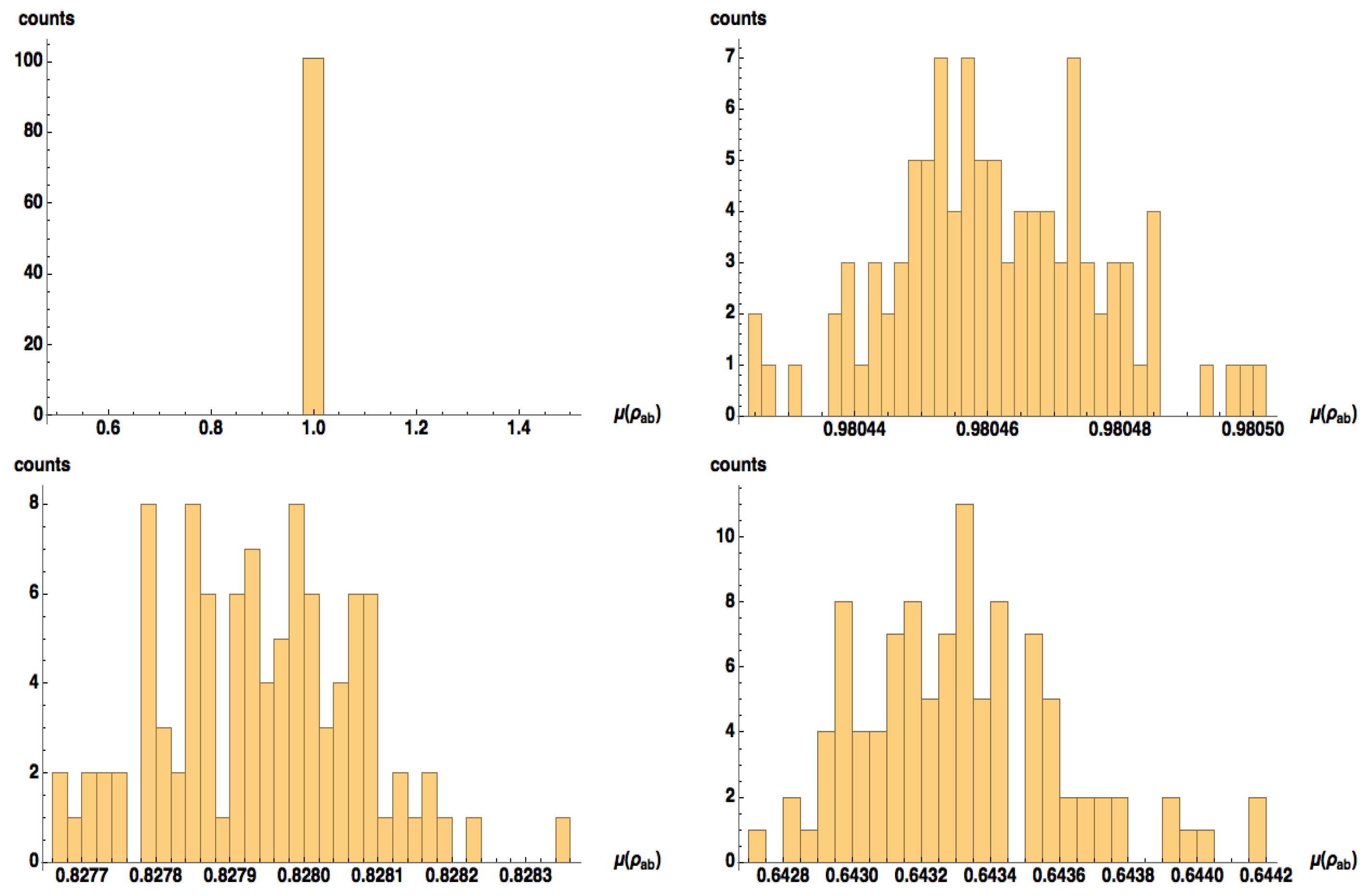
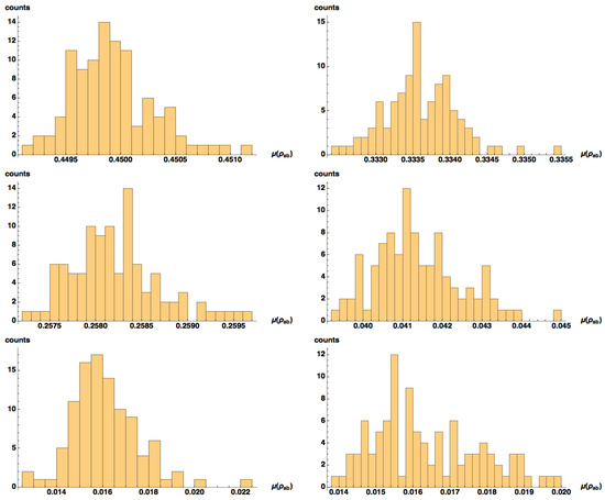
Figure A2.
Same as Figure A1, now with (top left) , (top right) , (middle left) , (middle right) (bottom left) , (bottom right) .
Figure A2.
Same as Figure A1, now with (top left) , (top right) , (middle left) , (middle right) (bottom left) , (bottom right) .

Appendix C. Description of Log Negativity Formulas Used in the Main Text
In this appendix, we describe the various Log Negativity formulas used in the main text, and for what type of states (density matrices , pure or mixed) they are applied to.
- Log Negativity for pure states
- —exact (subscript e) Log Negativity (), computed as the log of sum of the absolute values of the negative eigenvalues of the partial transpose of the pure state density matrix .
- —approximate (subscript a) Log Negativity (), computed by Equation (11b), with approximate Negativity computed in Equation (11a) from the wavefunction coefficients .
- Log Negativity formulas for general mixed states
- —exact Log Negativity, computed with the same corresponding definition above, except now is a general mixed state.
- , for
- —approximate Log Negativity computed for general mixed states with Equation (17c), with negativity computed with Equation (17b).
- , for
- Average approximate Log Negativity for mixed states written as pure state decompositions (PSDs) given by
- , using employing Equation (11a,b) on the pure state components .
Appendix D. Scaling of
The approximate Log Negativity formula Equation (11b) for pure states scales as [35], where is the dimension of the bipartite Hilbert space (since both n and m take values in the pure state ) as shown numerically in Figure A3. This scaling arises from the pair choices of indices n and m for the determinants that are calculated in the approximate negativity in Equation (11a). Note that a computation of the linear entropy scales like since it involves matrix–matrix multiplication to compute the reduce density matrix . In comparison, straightforward eigenvalue computation scales as [35], which could be reduced to on parallel architectures. While these scaling features show that the computation of an entanglement witness by means that do not involve eigenvalue computation hold some numerical advantage for large dimensions, it is not the primary emphasis or motivation for our investigation of the curious properties of the approximate Log Negativity.
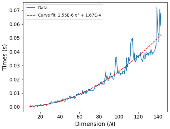
Figure A3.
Quadratic scaling of the approximate Log Negativity formula Equation (11b) in time (s) vs. the dimension of the bipartite Hilbert space for pure states .
Figure A3.
Quadratic scaling of the approximate Log Negativity formula Equation (11b) in time (s) vs. the dimension of the bipartite Hilbert space for pure states .

References
- Toth, G.; Apellaniz, I. Quantum metrology from quantum information science perspective. J. Phys. A Math. Theor. 2014, 47, 424006. [Google Scholar] [CrossRef]
- Report of the DOE Quantum Internet Blueprint Workshop. From Long-Distance Entanglement to Building a Nationwide Quantum Network. Available online: https://www.energy.gov/sites/prod/files/2020/07/f76/QuantumWkshpRpt20FINAL_Nav_0.pdf (accessed on 5 February 2020).
- Nielsen, M.A.; Chuang, I.L. Quantum Computation and Quantum Information; Cambridge University Press: Cambridge, UK, 2000. [Google Scholar]
- Schrödinger, E. Discussion of Probability Relations between Separated Systems. Math. Proc. Camb. Philos. Soc. 1935, 31, 555–563. [Google Scholar] [CrossRef]
- Schrödinger, E. Probability relations between separated systems. Math. Proc. Camb. Philos. Soc. 1936, 32, 446. [Google Scholar] [CrossRef]
- Einstein, A.; Podolsky, B.; Rosen, N. Can quantum-mechanical description of physical reality be considered complete. Phys. Rev. 1935, 47, 777. [Google Scholar] [CrossRef]
- Swingle, B. Spacetime from entanglement. Annu. Rev. Cond. Matt. Phys. 2017, 9, 345. [Google Scholar] [CrossRef]
- Horodecki, R.; Horodecki, P.; Horodecki, M.; Horodecki, K. Quantum Entanglement. Rev. Mod. Phys. 2009, 81, 865. [Google Scholar] [CrossRef]
- Bengtsson, I.; Zyczkowski, K. The Geometry of Quantum States, 2nd ed.; Cambridge University Press: Cambridge, UK, 2020. [Google Scholar]
- Wootters, W. Entanglement of Formation of an Arbitrary State of Two Qubits. Phys. Rev. Lett. 1998, 80, 2245. [Google Scholar] [CrossRef]
- Peres, A. Separability Criterion for Density Matrices. Phys. Rev. Lett. 1996, 77, 1413. [Google Scholar] [CrossRef]
- Horodecki, P. Separability criterion and inseparable mixed states with positive partial transposition. Phys. Lett. A 1997, 232, 333. [Google Scholar] [CrossRef]
- Agarwal, G.S. Quantum Optics; Cambridge University Press: Cambridge, UK, 2013. [Google Scholar]
- Meyer, D.; Wallach, N. Global entanglement in multi-particle systems. J. Math. Phys. 2002, 43, 4273. [Google Scholar] [CrossRef]
- Alsing, P.M.; Tison, C.C.; Schneeloch, J.S.; Birrittella, R.J.; Fanto, M.L. The distribution of density matrices at fixed purity for arbitrary dimensions. Phys. Rev. Res. 2022, 4, 043114. [Google Scholar] [CrossRef]
- Xie, S.; Younis, D.; Eberly, J.H. Evidence for unexpected robustness of multipartite entanglement against sudden death from spontaneous emission. Phys. Rev. Res. 2023, 5, L032015. [Google Scholar] [CrossRef]
- Eisert, J.; Brandão, F.G.; Audenaert, K.M. Quantitative entanglement witnesses. New J. Phys. 2007, 9, 46. [Google Scholar] [CrossRef]
- Ghühne, O.; Reimpell, M.; Werner, R.F. Estimating Entanglement Measures in Experiments. Phys. Rev. Lett. 2007, 98, 110502. [Google Scholar] [CrossRef]
- Ryu, S.; Lee, S.S.B.; Sim, H.S. Minimax optimization of entanglement witness operator for the quantification of three-qubit mixed-state entanglement. Phys. Rev. Lett. 2012, 86, 042324. [Google Scholar] [CrossRef]
- Aćin, A.; Tarrach, R.; Vidal, G. Optimal estimation of two-qubit pure-state entanglement. Phys. Rev. A 2000, 61, 062307. [Google Scholar] [CrossRef]
- Sancho, J.M.G.; Huelga, S.F. Measuring the entanglement of bipartite pure states. Phys. Rev. A 2000, 61, 042303. [Google Scholar] [CrossRef]
- Horodecki, P. Method for direct detection of quantum entanglement. Phys. Rev. Lett. 2002, 89, 127902. [Google Scholar] [CrossRef]
- Chen, K.; Albeverio, S.; Fei, S.M. Concurrence of arbitrary dimensional bipartite systems. Phys. Rev. Lett. 2005, 95, 040504. [Google Scholar] [CrossRef]
- Abanin, D.A.; Demler, E. Measuring entanglement entropy of a generic many-body system with a quantum switch. Phys. Rev. Lett. 2012, 109, 020504. [Google Scholar] [CrossRef]
- Karimi, N.; Heshmati, A.; Yahyavi, M.; Jafarizadeh, M.A.; Mohammadzadeh, A. Measurability of the D-concurrence. Sci. Rep. 2019, 9, 19415. [Google Scholar] [CrossRef] [PubMed]
- Meurice, Y. Lower bounds on entanglement entropy without twin copy. Phys. Rev. Res. 2025, 7, L022023. [Google Scholar] [CrossRef]
- Pauletti, T.; Silva, M.A.G.; Canella, G.A.; Franca, V.V. Linear entropy fails to predict entanglement behavior in low-density fermionic systems. Phys. A Stat. Mech. Its Appls. 2024, 644, 129824. [Google Scholar] [CrossRef]
- Morelli, S.; Klöckl, C.; Eltschka, C.; Siewert, J.; Huber, M. Dimensionally sharp inequalities for the linear entropy. Linear Algebra Its Appl. 2020, 584, 294–325. [Google Scholar] [CrossRef]
- Hill, S.A.; Wootters, W.K. Entanglement of a parit of quantum bits. Phys. Rev. Lett. 1997, 78, 5022. [Google Scholar] [CrossRef]
- Wootters, W.K. Entanglement of formation and concurrence. Quantum Inf. Comp. 2001, 1, 27. [Google Scholar] [CrossRef]
- Audenaert, K.; Verstraete, F.; Moor, B.D. Variational characterizations of separability and entanglement of formation. Phys. Rev. A 2001, 64, 052304. [Google Scholar] [CrossRef]
- Rungta, P.; Buzek, V.; Caves, C.M.; Hillery, M.; Milburn, G.J. Universal state inversion and concurrence in arbitrary dimensions. Phys. Rev. A 2001, 64, 042315. [Google Scholar] [CrossRef]
- Zyczkowski, K.; Horodecki, P.; Sanpera, A.; Lewenstein, M. Volume of the set of separable states. Phys. Rev. A 1998, 58, 883. [Google Scholar] [CrossRef]
- Mezzadri, F. How to generate random matrices from the classical compact groups. Not. AMS 2007, 54, 592. [Google Scholar]
- Press, W.H.; Teukolsky, S.A.; Vetterling, W.T.; Flannery, B.P. Numerical Recipes in C, 2nd ed.; Cambridge University Press: Cambridge, UK, 1992. [Google Scholar]
Disclaimer/Publisher’s Note: The statements, opinions and data contained in all publications are solely those of the individual author(s) and contributor(s) and not of MDPI and/or the editor(s). MDPI and/or the editor(s) disclaim responsibility for any injury to people or property resulting from any ideas, methods, instructions or products referred to in the content. |
© 2025 by the authors. Licensee MDPI, Basel, Switzerland. This article is an open access article distributed under the terms and conditions of the Creative Commons Attribution (CC BY) license (https://creativecommons.org/licenses/by/4.0/).

