An Easily Adopted Workflow for the Preparation, Filtration, and Quantification of Microplastic Standards

Abstract

Microplastic (MP) pollution poses an emerging environmental concern, yet current methods for isolation and quantification are often time-consuming, costly, and poorly adapted to real-world variability. In this study, a workflow for the preparation, filtration, and quantification of MP standards, emphasizing environmental relevance and methodological efficiency, was developed and evaluated. To address the scarcity of irregularly shaped MP standards, low-cost, environmentally representative standards were lab-prepared by grinding and sieving plastic sheets. These MPs were successfully categorized according to sizes up to ~250 μm and dyed for enhanced visibility. The filtration efficiency for two systems, a long-circuit pump (LC-pump) and a short-circuit vacuum (SC-vacuum), was compared. The SC-vacuum method demonstrated a more than 11-fold increase in filtration speed and higher MP recovery rates for both polystyrene and polypropylene standards. Ethanol-based solvents significantly improved MP dispersion and recovery for irregular shapes of the MPs, including polystyrene and polypropylene. Finally, a user-guided machine learning tool (Ilastik) was implemented for automated MP quantification. Ilastik showed a strong correlation with manual counting (r = 0.824) and reduced variability, offering a reproducible and time-efficient alternative. By cutting down cost, time, and technical complexity relative to existing MP analysis techniques, this workflow provides a more accessible path toward consistent and scalable environmental MP assessments.

1. Introduction

Microplastic (MP) particles are synthetic, hydrophobic particles between 1 μm and 5 mm, varying in size, shape, and composition [1,2,3,4,5]. They are pervasive and persistent pollutants that bioaccumulate in various environmental matrices and living organisms [6,7,8]. Health concerns are rising regarding MPs, as they have been identified in multiple human tissues [8]. Microplastic toxicity can stem from its ability to act as a vector for microorganisms, metals, and persistent organic pollutants [9,10].

The use of standardized MPs in research remains inconsistent due to the lack of reference materials, limiting reproducibility across studies [11]. Commercially available standards often include surfactants and have uniform shapes and sizes, which do not reflect the diversity of environmental MPs [11]. Spherical micro- and nanoplastics are used in nearly two-thirds of aquatic toxicity studies, despite the fact that they are seldom found in this form in the environment. Polystyrene (PS) and polyethylene (PE) are the most frequently used polymers in research, leading to their overrepresentation relative to other plastic types. Meanwhile, polypropylene (PP), though present in over 50% of freshwater and drinking water studies, is included in only 6% of studies evaluating biological effects [12]. Over the past decade, MP research has grown rapidly, resulting in a wide range of protocols tailored to specific matrices [13,14,15]. However, many of these methods involve lengthy separation steps and lack consistency in the size, shape, and polymer type of MPs. Other methodologies focus on larger particles (over 300 µm) and often use tedious steps, limiting their accessibility and replicability [11,16].

Currently, there are no fast and reliable counting methods for quantifying MPs [17]. Manual microscope-based counting remains the most common tool since it allows for the assessment of size, color, and shape, but it is time-consuming and subjective to the operator [13,17]. The most proficient way to analyze MPs’ polymer, type, and size counts is through spectroscopic methods like Fourier transform infrared (FTIR) and Raman spectroscopy combined with visual analysis tools [5]. However, such instruments are not readily available for all research groups, and analyzing the entire area of the filter is normally time-consuming (1~2 samples per day), urging the development of alternatives [16]. Open-source software like ImageJ, siMPle, System for Microplastics Automatic Counting and Classification (SMACC) [2,18,19,20], or machine-based learning algorithms [21,22] show promise in MP quantification. However, they have long initial processing times and are relatively new.

The general workflow for MP research focuses on four parts: sampling, extraction (filtration), characterization, and quantification [15]. These pre-quantification steps play a pivotal role in accurate MP analysis. Further research is needed to optimize the filtration of water samples, which is usually performed using a vacuum system with a Büchner flask [3,23,24,25,26]. Alternatively, pump-based filtration systems have also been employed in lab settings for microplastic extraction [27]. The lack of standardization in filtration methodology, coupled with extensive equipment requirements, points to a need for simple, homogenized, and replicable procedures that can be easily adopted across research groups [15].

Microplastics are known for their hydrophobic properties and non-polar surfaces, which increase their propensity for aggregation during filtration/extraction [28]. As the size of MPs decreases, their hydrophobicity and propensity to aggregate increase due to a higher surface area/volume ratio [28]. The majority of studies use water for their stock suspension [29], while others report using ethanol [13,28,29]. Studies using water-based solutions reported persistent aggregation of MPs mainly at the surface, while those that used alcohol-based solutions reported minimized MP aggregation and decreased density of particles compared to water, allowing for a more homogenous dispersion [28].

This study aims to establish a reproducible workflow for MP standard preparation, filtration, and quantification. We introduce a straightforward method for producing irregularly shaped polystyrene (PS) and polypropylene (PP) MPs in the <250 μm size range. The homogeneity and dispersion of the standard stock solutions were evaluated under varying ethanol concentrations. Using both commercially available and lab-prepared polymer standards, different filtration techniques were tested to identify the most effective method for maximizing MP recovery, alongside a comparison of different quantification tools to assess counting efficiency and accuracy.

2. Materials and Methods

2.1. Best Practices

To keep with best practices, a cotton overlay was worn at all times during wet lab procedures [29,30]. Gloves were not used for filtration methods as they can be a source of microplastic contamination. Instead, hands were washed and air-dried before all lab procedures. Before using any materials, all equipment was washed with tap water three times, once with deionized (DI) water, followed by a final wash of ethanol. All beakers were covered with aluminum foil to avoid contamination [2]. Prior to use, the surfaces of lab benches and fume hoods were wiped with a damp cotton cloth to eliminate settled dust and other particles. We adopted a methodology that minimizes the loss of MPs by limiting the number of container transfers and instead prioritized the use of larger-volume pipetting (10 mL serological pipettes or greater) for sample handling whenever transfer was required.

2.2. Development of Lab-Prepared MP Standards

Due to the limitations of the spherical commercially available standards, the creation of lab-prepared standards (Figure 1) was necessary to model irregular MP shapes found in real-world contexts. Lab-prepared MP standards were ground, sieved, and dyed to conduct MP counting.

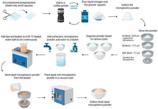
Figure 1. Preparation of environmentally relevant lab-prepared microplastics. The grinding and size separation process for creating microplastic standards with irregular shapes, along with the dyeing process of Rit DyeMore dye for coloring the lab-prepared microplastic.

2.2.1. Grinding Process

Figure 1 highlights the grinding and size separation process for creating MP standards with irregular shapes. Polystyrene (PS) (White Polystyrene 12” X 24” X .020” Plastic Sheet Styrene, purchased from Amazon.com Inc, USA) was cut into small squares. The PS squares were mechanically broken down in a coffee grinder (BCG111, KitchenAid, manufactured in China) and placed in aluminum containers, where they were immersed in liquid nitrogen for 3 min. This cooling process was repeated every 30 min between grinding runs to prevent overheating. The grinding process was also conducted with polypropylene (PP) (Up&Up 2-pocket blue portfolio, purchased from Target Brands Inc., Virginia, USA). The grinding process required a minimum of 5 h to achieve the largest target MP size (>250 μm) with an additional 5 h for every smaller size range desired.

2.2.2. Dry Sieving Process

Following the grinding, the MP pieces were dry sieved onto a stacked sieved system (Vonoso stainless steel mesh lab sieves, purchased from Amazon.com Inc., USA) to obtain three MP sizes: 60–80 mesh (~177–250 μm), 80–200 mesh (~77–177 μm), and 200 mesh (<77 μm). The sieving process required a minimum of 1 h to sieve all the MPs through one mesh size.

2.2.3. Dyeing Process

Three commercially available and cost-effective dyes—Rit DyeMore Synthetic Fiber Dye (Rit DyeMore, Nakoma Products, Apricot Orange, Item #01272-3100; Royal Purple, Item #01272-6410; Peacock Green, Item #01272-7530, Illinois, USA), Jacquard Piñata Color Alcohol Ink (Jacquard Products, Rupert, Gibbon & Spider, INC. item#019, California), and Jacquard iDye Poly for synthetic fibers (Jacquard Products, Rupert, Gibbon & Spider, INC. item#447, California, USA)—were tested on the lab-prepared polystyrene standard. The white color of the PS was not visible for imaging and counting purposes; however, the PP standard had blue coloration. These particular dyes were chosen because they were commercially available and affordable, concurring with the objective of this paper, and they were also used in prior research. For example, Karakolis et al. utilized 18 iDye Poly and 10 Rit DyeMore colors to label microplastics across seven plastic types; Hartig et al. applied Jacquard Piñata dyes to stain glass microspheres; and Tewari et al. employed yellow Jacquard iDye Poly on 22 different polymer types [29,31,32]. To assess dye suitability, all three were evaluated for color retention in ethanol-based suspensions. Of these, only Rit DyeMore Synthetic Fiber Dye retained its color under the tested conditions and was therefore used for dyeing the MP particles in this study. The optimized dyeing process, shown in Figure 1, requires a 93 °C (200 °F) water bath with a beaker of 200 mL of DI water mixed with 4 pumps of surfactant (89137-124, VWR), 3.52 g of dye, and up to 15 g of MPs of the desired size range. The solution was mixed consistently for one hour, and for the next hour, the solution settled in the water bath. On the smallest sieve size, the dyed MPs were rinsed with tap water until the water ran clear. The sieve was vertically tilted for the water to run through the underside to remove the MP pieces and have them drip into the aluminum container. The container was placed in a vacuum oven until the water fully evaporated, and the MPs were completely dried. All sizes were initially dyed orange. Later, for further analysis, to visually distinguish between the size fractions of the lab-prepared polystyrene (PS) standards, RIT DyeMore was applied in different colors: orange for particles <77 µm, purple for particles 77–177 µm, and green for particles 177–250 µm. Separate standard solutions were prepared for each size group, with 0.001 g/100 mL of <77 µm PS suspended in 50% ethanol and 0.002 g/100 mL for the two larger fractions also suspended in 50% ethanol. A sample of 10 mL was then filtered onto individual filter papers for counting and measuring the particle size.

2.3. Filtration Standard Operating Procedure

In preparation for filtration, both filtration methods described required the disassembled nozzle (AdvantecTM KS 13, Stainless Steel Syringe Holder, 13 mm (SKU: 301000, Sterlitech Corporation, Auburn, Washington USA)) to be soaked in DI water for 15 min. To clean the apparatus, DI water was gently swirled in the separatory funnel to capture all surfaces, followed by three backwashes. While cleaning the separatory funnel, the stopcock of the separatory funnel was opened and closed to allow DI water to flow. Afterward, the separatory funnel and nozzle were briefly washed with ethanol for a final flush. The filter was placed into the nozzle, and the separatory funnel was covered with aluminum foil.

To better accommodate the filtration apparatus setup, a Whatman^® filter paper (Whatman 3 qualitative, diameter 55 mm, 100 circles, purchased from Sigma-Aldrich (Cat No. 1003-055), USA) with a 5-micron porosity (cellulose filter) was customized. The filter was placed on a YKSPLUSK protective mat, and a hole-punching tool was used to cut the filter paper into a circle of 1/2 inch in diameter, then stored in a Petri dish covered in aluminum foil to avoid contamination.

In this study, two filtration methods, namely long-circuit pump (LC-pump) and short-circuit vacuum (SC-vacuum), were custom-built in the lab and assessed in terms of MP recovery and isolation efficiency as seen in Figure 2. In the LC-pump filtration method (Masterflex™ L/S™, purchased from Fisher Scientific (Catalog No. 13-200-008), USA), a separatory funnel containing the sample was pumped at a 6.0 rpm flow rate through a long-circuit Teflon tube of 96.5 cm (Viton FDA Tube 1/16” ID × 1/8” OD, purchased from Cole-Parmer, USA). The sample was run through the stainless-steel nozzle containing the filter. In the SC-vacuum filtration method, a separatory funnel was attached to the Büchner flask directly with a plastic connector tube of 6.9 cm in length to the stainless-steel nozzle. To complement the short circuit apparatus, a perforated stopcock connected to a Teflon tube with a length of 3 cm maintained the vacuum filtration suction and prevented sample leakage from the stainless-steel nozzle to the vacuum.

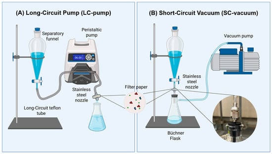
Figure 2. Custom-built filtration systems are used for microplastic isolation. (A) Long-circuit pump (LC-pump) filtration system. (B) Short-circuit vacuum (SC-vacuum) filtration system with a close-up of the stainless-steel nozzle unification to the Büchner flask.

To prepare the MP solution for filtration, the solvent containing MPs was shaken manually for 1 min to resuspend the MPs, and 20 mL was pipetted into the filtration apparatus. After filtration, the filter was transferred via forceps to the FTIR stage for imaging, covering the filter and keeping it horizontal during transfer.

Both filtration systems were tested with lab-prepared or commercially available MPs. A commercially available MP polymer, polypropylene (chromatographic grade polypropylene, purchased from PolySciences (04342-100), PA, USA) with a size range of 25–85 μm, was used in addition to lab-prepared polystyrene with a size range of 77–177 μm. The concentrations of MP solutions ranged from 11.2 to 13.3 μg/mL to limit the aggregation of MPs on the filters. Additionally, both methods were timed during filtration to measure the time it takes to filter the same standard volume.

2.4. Ethanol Effect on MP Dispersion

To evaluate the effect of ethanol concentrations on MP dispersion, a series of suspension solutions was prepared using PP and PS particles (sieved to 77–177 µm size). For each polymer type, 0.002 g of particles was added to 40 mL solutions at four concentrations: 0% (pure water), 20%, 50%, and 100% ethanol by volume. Each tube was capped and shaken manually for one minute to ensure initial dispersion, then left undisturbed for five minutes to allow settling. Photographs were taken immediately after settling to visually assess the degree of dispersion, floating behavior, and particle adherence to the water surface and inner tube walls. Next, we evaluated the effect of ethanol addition on MP counts after filtration. Three types of MP standards were used:

• Commercially available PS beads (Duke Standards™, 3 × 10⁴ particles/mL, 99 µm diameter, 12 particles/mL final concentration used after dilution, purchased from Fisher Scientific (Catalog No.09-980-216), USA)
• Lab-prepared PS standard (77–177 µm, 13.3 µg/mL)
• Lab-prepared PP standard (77–177 µm, 20.0 µg/mL)

For both the PS beads and lab-prepared PS, two solutions were prepared: one in 0% ethanol and one in 50% ethanol. For each condition, 20 mL of suspension was filtered to produce individual filters (n > 3). Similarly, for the lab-prepared PP standard, suspensions were prepared in 0% and 100% ethanol, and 10 mL from each was used per filter (n > 3). This approach allowed visual and quantitative comparison of the impact of ethanol on MP dispersion and recovery.

2.5. Quantification and Identification of MPs

2.5.1. FTIR, siMPle Analysis, and Scanning Electron Microscope (SEM)

To identify the polymer types of MPs and quantify them, analysis was conducted using the Nicolet iN10 Fourier-transform infrared (FTIR) microscope. Each filter was scanned with a mosaic image via CCD that covered approximately 80% of its effective area (128 × 128 points). Normally, the size of MP particles larger than ~70 μm was visible on the mosaic images. The FTIR settings for microplastic analysis included a cooled detector with a spectral range of 4000 to 1100 cm⁻¹, standard spectral resolution, and a collection time of 0.85 s (4 scans), equating to 3.18 s per point with a 50 μm step size. The total scan time for 80% of the filter’s effective area was approximately 16 h. The resulting spectral data were exported as ENVI files and analyzed using the Systematic Identification of Microplastics in the Environment (siMPle) software (Version 1.0.0), developed by Aalborg University and the Alfred Wegener Institute (https://simple-plastics.eu/). siMPle compares the acquired spectra with reference libraries to identify polymer types, count particles, and visualize their spatial distribution. Using this approach, polymer maps and concentration data were generated. To quantify MPs larger than 70 μm, a mosaic image of the filter was captured using the FTIR camera with a 50 μm step size over a 300 × 300-point grid, taking approximately 15 min. Particle counts were then obtained from the mosaic images.

To measure the particle sizes of the lab-prepared PS standard and morphological characterization, the size and surface morphology of the microplastics were examined by field emission scanning electron microscopy (FE-SEM) (Zeiss SUPRA55-VP, manufactured by Carl Zeiss Inc., Jena, Germany). Since microplastic particles larger than 100 μm tend to detach from metal stubs during imaging, a fixation method was used to improve adhesion and minimize aggregation. Specifically, 50 μL of a 1:10 ethanol-diluted Nafion™ perfluorinated resin solution (purchased from Sigma-Aldrich (510211), USA) was deposited onto the metal substrate, followed by the application of a small aliquot of the MP sample. The particles were gently dispersed within the droplet using a pipette tip to ensure uniform distribution before drying. As the ethanol evaporated, a thin Nafion film formed, effectively immobilizing the MPs. SEM imaging was conducted using a low accelerating voltage (5–10 kV) with the SE2 detector to minimize beam-induced damage. Particle dimensions were measured in ImageJ (Version 1.54g), with both the major axis (the longest possible line through the particle) and the minor axis (the longest line perpendicular to the major axis) recorded. These measurements were used to validate whether particle dimensions aligned with the mesh size criteria, since particles would pass through a mesh only if both axes were smaller than the mesh opening. Additionally, FTIR spectral analysis was performed using the Hummel Polymer Sample Library to confirm the polymer identity of the PS (Figure 3A) and PP (Figure 3B) used in the lab-prepared standards. The bands in 3150~3500 cm⁻¹ and 1650~1750 cm⁻¹ are from the stretching vibration of v(O-H) and v(C=O), respectively. The observation of these bands implies the oxidative degradation of the polymer during mechanical grinding. Other researchers also observed similar FTIR bands after processing PP [33].

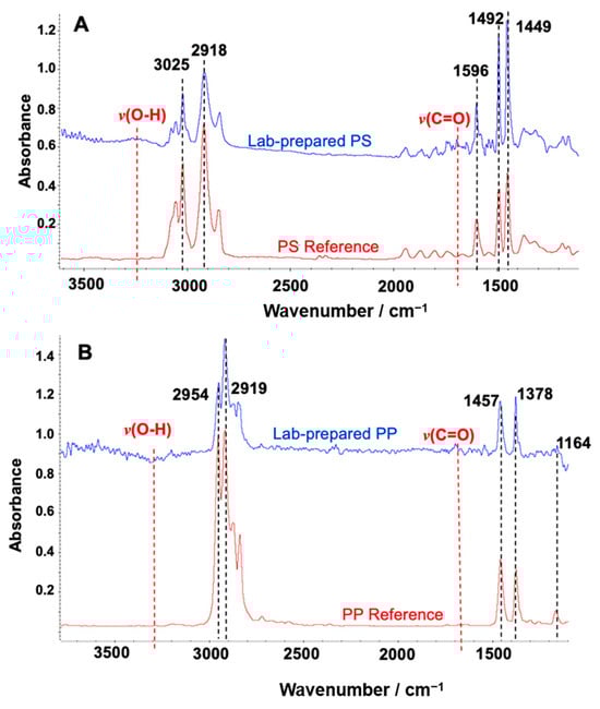
Figure 3. FTIR spectrum matches with Hummel Polymer Sample Reference Library. (A) Lab-prepared polystyrene (PS) (blue) and PS from the library (red); (B) lab-prepared polypropylene (PP) (blue) and PP from the library (red). The five most dominant matched peaks were marked by black dotted lines with the annotation of vibration frequencies. The red dotted line indicates the additional minor feature of IR peaks for v(O-H) and v(C=O), implying the oxidative degradation of the polymer during mechanical grinding.

2.5.2. Ilastik (v1.4.1)

Ilastik is an open-source machine-learning software that allows for algorithmic learning to segment, classify, track, and count image-based experimental data [34]. Pixel classification uses brushstrokes to assign different labels to pixels of features on an image based on using manual annotations. After the user annotations were set, the automated system returned a prediction and segmentation that was overlaid on each uploaded image. Merged features and mistakes were corrected with additional training, which could take four hours per project (given no change in variables in the experiment). However, after the project was fully trained, images could be analyzed in seconds, providing a scalable and fast alternative to manual counting. The identification of MPs with Ilastik reveals how it labels the MPs on the filter paper based on its user-guided pixel and object classification workflows. Briefly, filter images were annotated by the user for pixel areas identifying MPs or other objects in the image (training phase). Next, the regularity and size of each object to be included in further analyses were controlled in the thresholding phase. It was important to optimize a separate Ilastik workflow for each MP type, as training and thresholding varied significantly across MP types.

3. Statistical Methods

Statistical significance was determined when sample sizes were greater than or equal to n = 3. A p-value of < 0.05 was considered statistically significant. Bar chart data were presented as mean + standard deviation. Statistical analyses were performed using GraphPad Prism 10 (GraphPad Inc., La Jolla, CA, USA) unless otherwise noted. Graphical illustrations were designed by GraphPad Prism (Version 10) or BioRender.

4. Results and Discussion

Due to the high cost and limited availability of irregularly shaped MP reference materials that accurately represent environmental particles, we developed a cost-effective approach for generating MPs by manually fragmenting commercially available PS and PP sheets. To improve the homogeneity of MP suspensions and minimize particle loss resulting from adhesion to glassware, we evaluated the use of ethanol as a dispersing agent. A custom filtration apparatus was also designed and tested for compatibility with both lab-generated and commercially sourced MP standards. Furthermore, we established a time-efficient and reproducible quantification workflow by integrating artificial intelligence-based image analysis software to automate MP counting.

4.1. Preparation of Environmentally Relevant MP Standards

Lab-prepared polystyrene MP standards were mechanically broken down for fragmentation and dyed for visibility under microscopy (Figure 4) (see the Materials and Methods section for details). Sieving produced three size categories (<77 µm (orange), 77–177 µm (purple), and 177–250 µm (green)) of the lab-prepared polystyrene MPs according to the mesh size (Figure 4A). The optical images under FTIR microscopy are shown in Figure 4B, and selected SEM images are presented in Figure 4C. More SEM images can be found in the Supporting Information (Figures S1–S4). As shown in the SEM images, the ground polystyrene MPs are irregular in shape, representing MPs in the environment. Therefore, the length of the major axis, the longest dimension, and the minor axis, the shortest dimension, of each MP were measured for the particle size distribution statistics presented in Figure 4D. The minor axis ranged from 76 ± 21 µm at <77 µm, to 115 ± 42 µm at 77–177 µm, and 133 ± 52 µm at 177–250 µm. Similarly, the major axis ranged from 112 ± 31 µm to 167 ± 58 µm and 207 ± 96 µm across the same sieve mesh size categories. We noted some variation in particle size compared to mesh size, especially within the largest size range (177–250 μm). This discrepancy is likely attributable to the irregular geometry and non-spherical morphology of the manually generated particles (see Figure 4C and Figures S1–S4), which can lead to variable orientation and deformation during sieving. As a result, some particles with dimensions exceeding the mesh aperture in one axis may still pass through due to their alignment or flexibility. These observations underscore the challenges of size-fractionating the irregularly shaped MPs and highlight the need for complementary characterization methods beyond sieve-based classification, such as the mosaic image and SEM image confirmations shown in Figure 4B,C. In contrast to commercial MP standards that are typically expensive and sold in small quantities, our lab-prepared MPs from cryo-ground plastic sheets provide an extremely low-cost alternative suitable for high-volume experimental work.

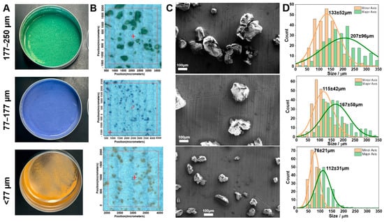
Figure 4. Microplastic (MP) size distribution of the lab-prepared polystyrene standard of different sizes. (A) Dyed lab-prepared polystyrene (PS). (B) FTIR microscopy mosaic images of the dyed lab-prepared PS polymer for size analysis (n > 3). The red cross indicates the midpoint of the selected location. (C) Selected scanning electron microscopy (SEM) images of sieved MPs with the same length of scale bar (n = 1). (D) Size distribution chart of MPs’ lengths of minor axis (orange) and major axis (green) from SEM images (~200 MPs analyzed) (n = 1).

4.2. Ethanol-Based Solvents Enhance the Recovery of MPs with Irregular Shapes

To enhance the MP dispersion in aqueous solution, we made the lab-prepared standard solution using different concentrations of ethanol. Water alone has been shown to be a poor dispersant for MPs, especially for low-density polymers such as polyethylene and polypropylene, which tend to float and aggregate due to their hydrophobic surfaces and lower densities [28]. This results in poor suspension stability and reduced recovery. Ethanol, on the other hand, improves dispersion by reducing surface tension and increasing the wettability of MP particles, significantly decreasing aggregation and flotation effects [13,28]. Furthermore, ethanol enhances the accuracy and reproducibility of particle size measurements, particularly in laser diffraction and turbidimetric methods, by producing monomodal distributions and lowering the coefficient of variation [28]. Given these advantages and the inconsistency reported across studies using water-based stock solutions [29], ethanol was selected to enhance the environmental relevance and methodological robustness of our MP standard preparation process. We monitored the dispersion of lab-prepared PP and PS MPs using four ethanol concentrations (0%, 20%, 50%, and 100%) and indicated visible floating MPs (Figure 5A). The optimal dispersion without floating MPs and with minimal adherence to glassware was observed with >50% ethanol for lab-prepared PS standards and 100% ethanol for lab-prepared PP standards (Figure 5A). To further validate these findings, a comparative recovery analysis with three or more replicates was performed using the SC-vacuum method of filtration (see the Materials and Methods section). A comparison of a normalized count for the number of MPs in an ethanol-free solution (−) and with ethanol (+, 50% for PS and 100% ethanol for PP), along with the commercial PS beads standard, can be seen in Figure 5B. The PS beads in an ethanol-containing solution showed a moderate reduction in counts compared to those in an ethanol-free solution. However, lab-prepared PP and PS MPs in ethanol-containing solutions had significantly higher counts (1554% for PP and 140% for PS) than those in ethanol-free solutions (normalized to be 100%). It suggests a preferential advantage of ethanol for MPs with irregular shapes (Figure 5B). These results highlight the critical role of ethanol in enhancing dispersion and minimizing particle loss due to surface adhesion. It is also important to note that the lab-prepared PP and PS MPs were already colored in contrast to the commercial PS beads standard (no color), so whether uncolored PP and PS MPs with irregular shapes would also benefit from ethanol addition remains elusive. Microplastic contaminants in nature can be found in transparent or colored states, with the colored state correlating with higher degradation and MP formation [35]. While this study focused on standard preparation, the findings support a broader recommendation for researchers in the field. Ethanol should be considered not only during standard preparation but also during the cleaning of glassware and resuspension of samples, particularly after digestion and density separation steps used in environmental MP isolation protocols. Incorporating ethanol at these stages may improve recovery efficiency, reduce aggregation, and enhance the reproducibility of results in complex environmental matrices.

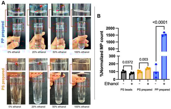
Figure 5. The recovery advantage of ethanol addition to the microplastic (MP) solution. (A) Representative images of the suspension standard in glass tubes of lab-prepared polypropylene (PP) and polystyrene (PS) standard. The dashed box refers to the zoomed area of the top part of the tube or a different view of it. (B) Comparison of normalized count for the number of microplastics in ethanol-free solution (−) and with ethanol (+, 50% for PS and 100% ethanol for PP). The average counts in ethanol-free solution for 3 or 4 replicates were assumed to be 100% for the comparison (n ≥ 3). The p-values between ethanol-free and with ethanol are shown on the bars.

4.3. Short-Circuit Vacuum Filtration Is Superior to Long-Circuit Pump Filtration in Terms of MP Counts

Two of the most common methods for MP filtration are pump and vacuum-based. We have designed two different systems utilizing the described methods, named long-circuit pump (LC-pump) and short-circuit vacuum (SC-vacuum) (see the Materials and Methods section and Figure 2). In comparing time efficiencies of each of the systems, we found that the average filtration time for the LC-pump method was 319 ± 3 s for a 20 mL standard solution, translating to a rate of approximately 3.8 mL/min (n = 6). In contrast, the SC-vacuum method filtered the same standard volume in 27 ± 1.5 s, or 44 mL/min (n = 24), resulting in over an 11-fold improvement in filtration speed. This substantial increase in efficiency suggests that the SC-vacuum setup is the more practical option for a broader application, which is a critical factor when evaluating scalability and feasibility for routine or large-scale sampling.

An illustration of the efficient isolation and quantification of MPs using FTIR microscopy analysis and manual counting in samples is shown in Figure 6A, where the SC-vacuum method (bottom) resulted in better dispersion of PS MPs on the filter, while the LC-pump method (top) resulted in MP aggregates. Microplastics that are clustered in aggregates can make counting individual particles challenging because of the overlap of individual particles. Most importantly, the SC-vacuum method resulted in significantly higher counts of lab-prepared PS MPs (77–177 μm) compared to the LC-pump method (133% compared to LC-pump, Figure 6A,B). Nevertheless, for the commercial PP beads standard (25–85 μm), the SC-vacuum method resulted in a 16-fold increase in MP counts compared to the LC-pump method (Figure 6C,D). These results indicate that the SC-vacuum method offers superior performance in terms of both processing efficiency and MP quantification. This enhanced recovery may be partly attributed to the shorter and more direct fluid pathway in the SC-vacuum configuration, which minimizes particle loss due to adhesion within the system. In contrast, the LC-pump method involves extended tubing and a more complex flow path, increasing the likelihood of MPs adhering to internal surfaces, particularly in the case of smaller or hydrophobic particles. Additionally, the reduced turbulence and more consistent suction in the SC-vacuum system may further contribute to improved particle capture and filter deposition.

Figure 6. Optimizing the filtration method for better microplastic (MP) isolation and quantification. (A) Representative images of filters capturing the filtered lab-prepared polystyrene (PS) microplastics (77–177 μm, 13.3 μg/mL) using long-circuit pump (LC-pump) and short-circuit vacuum (SC-vacuum) methods; the scale bar is 500 µm (n ≥ 4). (B) Normalized count of the number of PS microplastics detected (in A) for both methods using imaging-based counting (n ≥ 3), and normalized the counts of the LC-pump method to 100% (n ≥ 3). (C) Representative siMPle maps of filters capturing the commercial polypropylene (PP) microplastic beads (25–85 μm, 11.2 μg/mL) using both methods (n ≥ 3). (D) Normalized count of the number of PP microplastics detected (in C) for both methods using FTIR spectra-based counting (n = 4). The p-values between the two methods are shown on the bars.

4.4. User-Guided Machine Learning Analysis and Quantification of MPs

A comparison of manual and machine learning quantification of MPs after filtration using multiple samples of each specific polymer is illustrated in Figure 7. Specifically, Figure 7A shows counts for commercially available PS bead MPs. By plotting each paired manual and Ilastik quantification in Figure 7B, it illustrates that the Ilastik quantification had a moderately lower reported number of MPs than the manual quantification, except for 3 of the 31 filter counts. Figure 7C displays the 5 representative quantifications of both methods. The smaller deviation of quantification from Ilastik compared to manual quantification was also indicated, which underscores the machine’s consistency across different images. To address whether Ilastik quantification was correlated to manual quantification, all 31 counts from both methods were plotted versus each other in Figure 7D. The factor of Pearson product–moment correlation coefficient is 0.824, suggesting that the counts of both methods increase with each other. The linear regression produced a slope of 0.89, suggesting a strong but not perfect agreement between the two methods. While the slope approaches unity, which would indicate a one-to-one correspondence, the deviation from 1.0 implies a systematic difference in quantification between the methods. This may be due to differences in human/machine sensitivity in dealing with particle morphology, such as particle aggregates or closely packed particles. Therefore, it seems that both methods are broadly comparable (Figure 7D). These results indicate that Ilastik quantification can be used as an alternative to manual quantification, given proper training as described in the methods. Ilastik offers a streamlined workflow, requiring less than 4 h of initial training on a subset of filters, after which additional filter images can be processed and quantified within seconds, providing consistent and reproducible results. Due to the time-consuming nature and potential bias of manually quantifying MPs after filtration, an alternative approach using Ilastik machine learning may be a favorable choice. Relative to existing methods, our method (microscopy image and Ilastik counting) delivers a more streamlined and accessible counting process. It reduces the complexity of ImageJ-based pipelines, avoids the high cost and labor requirements of SEM, FTIR, and Raman systems, and cuts analysis time substantially compared with manual microscopy counting.

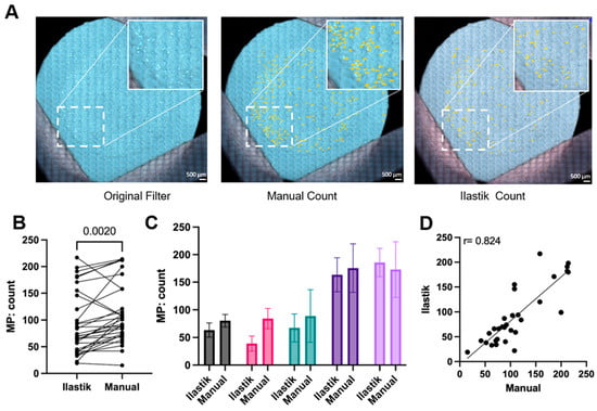
Figure 7. Ilastik quantification is a reliable alternative for manual quantification of microplastics (MPs). (A) Representative images of commercially available polystyrene (PS) microplastics filter with manual counting and Ilastik counting, as highlighted, the white box represents a magnified part of the filter (n = 31). The scale bar is 500 µm. (B) Paired microplastics count between Ilastik and manual quantification for different polymer shapes (spherical and irregular) and polymer sources: commercial (99 µm) or lab-prepared (77–177 µm), a paired t-test was used for statistical analysis (n = 31). (C) Pairwise analysis of microplastic counts from (B) presented as mean with standard deviation (n > 3). (D) Correlation analysis of pairwise counts from (B) with a simple linear regression fit line; correlation p-value is <0.0001 (n = 31).

5. Conclusions

This study presents a reproducible, scalable, and cost-effective workflow for the preparation, filtration, and quantification of environmentally relevant MP standards. By lab-preparing irregularly shaped PS and PP MPs and optimizing ethanol concentrations to improve dispersion, we addressed critical limitations in standard availability and particle aggregation. The short-circuit vacuum (SC-vacuum) filtration system significantly outperformed the long-circuit pump (LC-pump) method in both recovery efficiency and processing time, offering practical advantages for high-throughput applications. Additionally, the integration of a user-guided machine learning platform, Ilastik, provided a reliable, rapid, and less labor-intensive alternative to manual quantification, with a strong correlation between the two methods. Collectively, our findings support a simplified and effective pipeline that can be readily adopted by laboratories lacking access to high-cost instruments or commercial MP standards. This workflow enhances reproducibility, minimizes particle loss, and accommodates the physical diversity of MPs observed in environmental samples. The approach holds promise for standardizing MP research methodologies and facilitating broader participation in microplastics monitoring and impact assessment across disciplines.

References

- Enders, K.; Lenz, R.; Ivar do Sul, J.A.; Tagg, A.S.; Labrenz, M. When Every Particle Matters: A QuEChERS Approach to Extract Microplastics from Environmental Samples. MethodsX 2020, 7, 100784. [Google Scholar] [CrossRef]
- Primpke, S.; Cross, R.K.; Mintenig, S.M.; Simon, M.; Vianello, A.; Gerdts, G.; Vollertsen, J. Toward the Systematic Identification of Microplastics in the Environment: Evaluation of a New Independent Software Tool (siMPle) for Spectroscopic Analysis. Appl. Spectrosc. 2020, 74, 1127–1138. [Google Scholar] [CrossRef]
- Yang, J.; Monnot, M.; Sun, Y.; Asia, L.; Wong-Wah-Chung, P.; Doumenq, P.; Moulin, P. Microplastics in Different Water Samples (Seawater, Freshwater, and Wastewater): Methodology Approach for Characterization Using Micro-FTIR Spectroscopy. Water Res. 2023, 232, 119711. [Google Scholar] [CrossRef] [PubMed]
- Koelmans, A.A.; Mohamed Nor, N.H.; Hermsen, E.; Kooi, M.; Mintenig, S.M.; De France, J. Microplastics in Freshwaters and Drinking Water: Critical Review and Assessment of Data Quality. Water Res. 2019, 155, 410–422. [Google Scholar] [CrossRef]
- Primpke, S.; Wirth, M.; Lorenz, C.; Gerdts, G. Reference Database Design for the Automated Analysis of Microplastic Samples Based on Fourier Transform Infrared (FTIR) Spectroscopy. Anal. Bioanal. Chem. 2018, 410, 5131–5141. [Google Scholar] [CrossRef] [PubMed]
- Wang, F.; Feng, X.; Liu, Y.; Adams, C.A.; Sun, Y.; Zhang, S. Micro(Nano)Plastics and Terrestrial Plants: Up-to-Date Knowledge on Uptake, Translocation, and Phytotoxicity. Resour. Conserv. Recycl. 2022, 185, 106503. [Google Scholar] [CrossRef]
- Ziani, K.; Ioniță-Mîndrican, C.-B.; Mititelu, M.; Neacșu, S.M.; Negrei, C.; Moroșan, E.; Drăgănescu, D.; Preda, O.-T. Microplastics: A Real Global Threat for Environment and Food Safety: A State of the Art Review. Nutrients 2023, 15, 617. [Google Scholar] [CrossRef] [PubMed]
- Nihart, A.J.; Garcia, M.A.; El Hayek, E.; Liu, R.; Olewine, M.; Kingston, J.D.; Castillo, E.F.; Gullapalli, R.R.; Howard, T.; Bleske, B.; et al. Bioaccumulation of Microplastics in Decedent Human Brains. Nat. Med. 2025, 31, 1114–1119. [Google Scholar] [CrossRef]
- Prüst, M.; Meijer, J.; Westerink, R.H.S. The Plastic Brain: Neurotoxicity of Micro- and Nanoplastics. Part. Fibre Toxicol. 2020, 17, 24. [Google Scholar] [CrossRef]
- Gerdes, Z.; Ogonowski, M.; Nybom, I.; Ek, C.; Adolfsson-Erici, M.; Barth, A.; Gorokhova, E. Microplastic-Mediated Transport of PCBs? A Depuration Study with Daphnia Magna. PLoS ONE 2019, 14, e0205378. [Google Scholar] [CrossRef]
- Parker, L.A.; Höppener, E.M.; van Amelrooij, E.F.; Henke, S.; Kooter, I.M.; Grigoriadi, K.; Nooijens, M.G.A.; Brunner, A.M.; Boersma, A. Protocol for the Production of Micro- and Nanoplastic Test Materials. Microplast. Nanoplast. 2023, 3, 10. [Google Scholar] [CrossRef]
- de Ruijter, V.N.; Redondo-Hasselerharm, P.E.; Gouin, T.; Koelmans, A.A. Quality Criteria for Microplastic Effect Studies in the Context of Risk Assessment: A Critical Review. Environ. Sci. Technol. 2020, 54, 11692–11705. [Google Scholar] [CrossRef]
- Qin, X.; Teng, W.; Zhang, X.; Yang, Y.; Zhu, Y.; Liu, Z.; Li, W.; Dong, H.; Qiang, Z.; Zeng, J.; et al. Ethanol-Diluted Turbidimetry Method for Rapid and Accurate Quantification of Low-Density Microplastics in Synthetic Samples. Anal. Chim. Acta 2023, 1278, 341712. [Google Scholar] [CrossRef]
- Masura, J.; Baker, J.; Foster, G.; Arthur, C. Laboratory Methods for the Analysis of Microplastics in the Marine Environment: Recommendations for Quantifying Synthetic Particles in Waters and Sediments; Report; NOAA Marine Debris Division: Silver Spring, MD, USA, 2015. [Google Scholar] [CrossRef]
- Rani, M.; Ducoli, S.; Depero, L.E.; Prica, M.; Tubić, A.; Ademovic, Z.; Morrison, L.; Federici, S. A Complete Guide to Extraction Methods of Microplastics from Complex Environmental Matrices. Molecules 2023, 28, 5710. [Google Scholar] [CrossRef] [PubMed]
- Huppertsberg, S.; Knepper, T.P. Instrumental Analysis of Microplastics—Benefits and Challenges. Anal. Bioanal. Chem. 2018, 410, 6343–6352. [Google Scholar] [CrossRef]
- Lin, J.; Liu, H.; Zhang, J. Recent Advances in the Application of Machine Learning Methods to Improve Identification of the Microplastics in Environment. Chemosphere 2022, 307, 136092. [Google Scholar] [CrossRef]
- Valente, T.; Ventura, D.; Matiddi, M.; Sbrana, A.; Silvestri, C.; Piermarini, R.; Jacomini, C.; Costantini, M.L. Image Processing Tools in the Study of Environmental Contamination by Microplastics: Reliability and Perspectives. Environ. Sci. Pollut. Res. 2023, 30, 298–309. [Google Scholar] [CrossRef] [PubMed]
- Lorenzo-Navarro, J.; Castrillon-Santana, M.; Santesarti, E.; De Marsico, M.; Martinez, I.; Raymond, E.; Gomez, M.; Herrera, A. SMACC: A System for Microplastics Automatic Counting and Classification. IEEE Access 2020, 8, 25249–25261. [Google Scholar] [CrossRef]
- Vermeiren, P.; Muñoz, C.; Ikejima, K. Microplastic Identification and Quantification from Organic Rich Sediments: A Validated Laboratory Protocol. Environ. Pollut. 2020, 262, 114298. [Google Scholar] [CrossRef]
- Weber, F.; Zinnen, A.; Kerpen, J. Development of a Machine Learning-Based Method for the Analysis of Microplastics in Environmental Samples Using µ-Raman Spectroscopy. Microplast. Nanoplast. 2023, 3, 9. [Google Scholar] [CrossRef]
- Kedzierski, M.; Falcou-Préfol, M.; Kerros, M.E.; Henry, M.; Pedrotti, M.L.; Bruzaud, S. A Machine Learning Algorithm for High Throughput Identification of FTIR Spectra: Application on Microplastics Collected in the Mediterranean Sea. Chemosphere 2019, 234, 242–251. [Google Scholar] [CrossRef]
- Kim, J.; Kwon, J.; Kwon, J.; Siddiqui, M.Z.; Woo, G.; Choi, M.; Hong, S.; Ma, C.; Kumagai, S.; Watanabe, A.; et al. A New Filtration System for Extraction and Accurate Quantification of Microplastics. Anal. Methods 2024, 16, 6751–6758. [Google Scholar] [CrossRef]
- Gewert, B.; Ogonowski, M.; Barth, A.; MacLeod, M. Abundance and Composition of near Surface Microplastics and Plastic Debris in the Stockholm Archipelago, Baltic Sea. Mar. Pollut. Bull. 2017, 120, 292–302. [Google Scholar] [CrossRef] [PubMed]
- Use and Development of the Microparticle Sample Preparation Kit; Thermo Fisher Scientific: Waltham, MA, USA, 2025; Available online: https://assets.thermofisher.com/TFS-Assets/MSD/Technical-Notes/TN53168-use-development-microparticle-sample-preparation-kit.pdf (accessed on 10 September 2024).
- Schlawinsky, M.; Santana, M.F.M.; Motti, C.A.; Martins, A.B.; Thomas--Hall, P.; Miller, M.E.; Lefèvre, C.; Kroon, F.J. Improved Microplastic Processing from Complex Biological Samples Using a Customized Vacuum Filtration Apparatus. Limnol. Oceanogr. Methods 2022, 20, 553–567. [Google Scholar] [CrossRef]
- Harrold, Z.; Arienzo, M.M.; Collins, M.; Davidson, J.M.; Bai, X.; Sukumaran, S.; Umek, J. A Peristaltic Pump and Filter-Based Method for Aqueous Microplastic Sampling and Analysis. ACS EST Water 2022, 2, 269–278. [Google Scholar] [CrossRef]
- Fang, Z.; Sallach, J.B.; Hodson, M.E. Ethanol, Not Water, Should Be Used as the Dispersant When Measuring Microplastic Particle Size Distribution by Laser Diffraction. Sci. Total Environ. 2023, 902, 166129. [Google Scholar] [CrossRef]
- Tewari, A.; Almuhtaram, H.; McKie, M.J.; Andrews, R.C. Microplastics for Use in Environmental Research. J. Polym. Environ. 2022, 30, 4320–4332. [Google Scholar] [CrossRef]
- Kiefer, T.; Knoll, M.; Fath, A. Comparing Methods for Microplastic Quantification Using the Danube as a Model. Microplastics 2023, 2, 322–333. [Google Scholar] [CrossRef]
- Karakolis, E.G.; Nguyen, B.; You, J.B.; Rochman, C.M.; Sinton, D. Fluorescent Dyes for Visualizing Microplastic Particles and Fibers in Laboratory-Based Studies. Environ. Sci. Technol. Lett. 2019, 6, 334–340. [Google Scholar] [CrossRef]
- Hartig, J.; Howard, H.C.; Stelmach, T.J.; Weimer, A.W. DEM Modeling of Fine Powder Convection in a Continuous Vibrating Bed Reactor. Powder Technol. 2021, 386, 209–220. [Google Scholar] [CrossRef]
- Case Study: FTIR for Identification of Contamination. Jordi Labs, Mark Jordi. 2014. Available online: https://jordilabs.com/wp-content/uploads/2014/09/Case_Study_FTIR_For_Identification_Of_Contamination.pdf (accessed on 9 December 2024).
- Berg, S.; Kutra, D.; Kroeger, T.; Straehle, C.N.; Kausler, B.X.; Haubold, C.; Schiegg, M.; Ales, J.; Beier, T.; Rudy, M.; et al. Ilastik: Interactive Machine Learning for (Bio)Image Analysis. Nat. Methods 2019, 16, 1226–1232. [Google Scholar] [CrossRef] [PubMed]
- Key, S.; Ryan, P.G.; Gabbott, S.E.; Allen, J.; Abbott, A.P. Influence of Colourants on Environmental Degradation of Plastic Litter. Environ. Pollut. 2024, 347, 123701. [Google Scholar] [CrossRef] [PubMed]
Disclaimer/Publisher’s Note: The statements, opinions and data contained in all publications are solely those of the individual author(s) and contributor(s) and not of MDPI and/or the editor(s). MDPI and/or the editor(s) disclaim responsibility for any injury to people or property resulting from any ideas, methods, instructions or products referred to in the content. |
© 2026 by the authors. Licensee MDPI, Basel, Switzerland. This article is an open access article distributed under the terms and conditions of the Creative Commons Attribution (CC BY) license.