Breather and Rogue Wave Solutions of a New Three-Component System of Exactly Solvable NLEEs

Abstract

We derive a new exactly solvable multi-component system of non-linear evolution equations (NLEEs). The system consists of three $1+1$-dimensional evolution equations—one first-order and two second-order in the spatial variable. We review their Lax representation, formulate the scattering problem, and derive the soliton-like solutions of the system.

1. Introduction

Multi-component non-linear evolution equations (NLEEs) arise naturally as generalizations of famous equations of mathematical physics, like, for example, the non-linear Schrödinger equation (NLS) and the Korteweg–de Vries (KdV) and the modified KdV (mKdV) equations. Multi-component mKdV-type equations were studied extensively in [1,2]. Most of the low-dimensional cases were presented there, with some recent additions being available in [3,4,5]. Multi-component NLS-type equations are usually connected to symmetric spaces [6,7,8]. Some of the more famous multi-component NLS-type equations include the Manakov model [9] and spin 1 Bose–Einstein condensate [10]. Athorne and Fordy showed that a large class of multi-component KdV and mKdV equations can also be related to symmetric spaces [11]. Another example is given by the N-wave equations, which model the resonance interaction of wave packets in non-linear media [12,13,14,15].

All of the above examples are based on the generalized Zaharov–Shabat system (also called the Caudrey–Beals–Coifman system) [16,17,18,19,20,21]; i.e., they are related to a Lax pair with an L operator linear in the spectral parameter $\lambda$. We note that systems of this type are still actively studied; see for example [22,23,24,25]. One way to generalize such systems is to consider polynomial dependence in $\lambda$. Classical examples include the derivative NLS equations—the Kaup–Newell [26], Chen–Lee–Liu [27], and Gerdjikov–Ivanov models. Note that they are all examples of one-component NLEEs related to higher-order energy-dependent Lax operators [28,29]. While there have been some recent advances for multi-component systems (see for example [30]), the majority of cases remain unexplored. This article is a study in exactly this direction. We will derive a system of NLEEs related to a Lax pair, where L is third-order in $\lambda$ and M is fifth-order. The system takes the form

$$\begin{array}{cc}\hfill {\displaystyle \frac{\partial q_3}{\partial t}}& ={\displaystyle \frac{\partial q_1}{\partial x}}+{\displaystyle \frac{1}{2}}{q}_3^2{\displaystyle \frac{\partial q_3}{\partial x}}-2q_2{q}_1{q}_3-{\displaystyle \frac{1}{4}}{q}_2{q}_3^4-q_2^3,\hfill \\ \hfill {\displaystyle \frac{\partial q_2}{\partial t}}& ={\displaystyle \frac{1}{2}}{\displaystyle \frac{{\partial }^2{q}_3}{\partial x^2}}+{\displaystyle \frac{1}{2}}{q}_3^2{\displaystyle \frac{\partial q_2}{\partial x}}+2q_1^2{q}_3+{\displaystyle \frac{5}{4}}{q}_1{q}_3^4+q_1{q}_2^2+{\displaystyle \frac{1}{8}}{q}_3^7+{\displaystyle \frac{1}{2}}{q}_3^3{q}_2^2,\hfill \\ \hfill {\displaystyle \frac{\partial q_1}{\partial t}}& =-{\displaystyle \frac{1}{2}}{\displaystyle \frac{{\partial }^2{q}_2}{\partial x^2}}-{\displaystyle \frac{1}{2}}{\displaystyle \frac{\partial }{\partial x}}\left(2q_3^2{q}_1+{\displaystyle \frac{1}{4}}{q}_3^5+q_3{q}_2^2\right).\hfill \end{array}$$

(1)

It is exactly solvable by the inverse scattering method. In this paper we briefly outline the key moments in the formulation of the scattering problem—we properly define the fundamental analytic solutions (FASs) and their regions of analyticity based on the spectrum of the L operator. For an introduction to the theory of the FASs in the context of integrable models, see the classical papers of Shabat [31,32]. The FASs are connected to a (multiplicative) Riemann–Hilbert problem (RHP) with canonical normalization. An interesting thing to note is that one can start from an RHP directly and then derive the corresponding Lax representation. Such approach was used, for example, in [33]. Note that the same approach can also be used to derive multi-dimensional systems, but the related RHP in this case is non-local [34]. For an introduction to the application of the RHP in integrable models and the related history, we recommend [35].

We also present some soliton-like solutions to the NLEEs. They are derived using the Zakharov–Shabat dressing method (we recommend reading the classical paper [17], with some more recent exposition found in [36]). The system has at least two types of nontrivial solutions. The first type is given by breather waves—the solution is spatially confined, with the three components moving together. The other type of solution is a rogue wave—it is localized in time. In our case, this type of solution is not spatially confined. A review on different types of non-linear waves (including breathers and rogue waves) can be found in [37].

A note on terminology—when we say Lax pair, we assume that it is in the zero curvature representation (ZCR). Usually, Lax operators are scalars and do not contain a spectral parameter [38]. For example, the KdV equation

$${\displaystyle \frac{\partial }{\partial t}}u=6u{\displaystyle \frac{\partial }{\partial x}}u-{\displaystyle \frac{{\partial }^3}{\partial x^3}}u,$$

(2)

is a result of the Lax equation

$${\displaystyle \frac{\partial }{\partial t}}L=\left[P,L\right],$$

(3)

where

$$\begin{array}{cc}\hfill L& =-{\partial }_x^2+u,\hfill \\ \hfill P& =-4{\partial }_x^3+6u{\partial }_x+3{\partial }_{x}u.\hfill \end{array}$$

(4)

In the ZCR the Lax operators are first-order but no longer scalar:

$$\begin{array}{cc}\hfill L& =i{\partial }_x+\mathcal{U}(x,t,\lambda ),\hfill \\ \hfill M& =i{\partial }_t+\mathcal{V}(x,t,\lambda ),\hfill \end{array}$$

(5)

where $\mathcal{U}(x,t,\lambda ),\mathcal{V}(x,t,\lambda )$ are in general $n\times n$ matrices. The parameter $\lambda$ is called the spectral parameter. We can interpret L and M as connections (covariant derivatives) on some properly chosen manifold, with $\mathcal{U}(x,t,\lambda ),\mathcal{V}(x,t,\lambda )$ being the connection coefficients. Then the condition $\left[L,M\right]=0$ (which now plays the role of (3)) implies zero curvature on that manifold, hence the name ZCR. An introduction to Lax pairs and the zero curvature representation can be found in [39]. Also, an excellent introduction to the theory of Lax pairs and integrable models in general can be found in [40]. As an introduction to the inverse scattering method in the context of integrable systems, we recommend [41,42,43].

This paper is structured as follows: In Section 2 we review some preliminary material fixing the notations we will use. Section 3 considers the Lax representation and the derivation of the NLEEs. By imposing the zero curvature condition for the two operators of the pair, we derive the recursion relations, and by solving them we find the system of NLEEs. Section 4 is devoted to the formulation of the scattering problem for the Lax pair. We present the Jost solutions for the L operator, and we define the fundamental analytic solutions (FASs). We show that the FASs are related to a Riemann–Hilbert problem. We end the section by introducing the scattering data and finding its time evolution. Section 5 examines the soliton-like solutions of the NLEEs by using the dressing method. In Section 6 we conclude with a brief discussion.

2. Preliminaries

This section contains some very basic preliminaries from the basic theory of Lie algebras. If the reader is further interested, we recommend [44,45,46].

The simple Lie algebra $A_1\simeq sl(2,\mathbb{C})$ is the linear space of $2\times 2$ matrices with the operation $[,]$, called the commutator, defined by

$$\left[X,Y\right]=XY-YX,$$

(6)

for every $X,Y\in A_1$. Elements of the algebra are called generators. Note that for every $X\in sl(2,\mathbb{C})$, we have that $e^X$ is an invertible matrix with determinant 1. The set of these matrices forms a group under matrix multiplication, which is denoted by $SL(2,\mathbb{C})$. By matrix exponentiation we mean

$$e^X=\sum _{n=0}^{\infty }{\displaystyle \frac{X^n}{n!}}.$$

(7)

As a basis of $sl(2,\mathbb{C})$ we will use the Pauli matrices:

$${\sigma }_1=\left(\begin{array}{cc}0& 1\\ 1& 0\end{array}\right),{\sigma }_2=\left(\begin{array}{cc}0& -i\\ i& 0\end{array}\right),{\sigma }_3=\left(\begin{array}{cc}1& 0\\ 0& -1\end{array}\right).$$

(8)

They satisfy

$$\left[{\sigma }_j,{\sigma }_k\right]=2i{\epsilon }_{jkl}{\sigma }_l$$

(9)

with ${\epsilon }_{jkl}$ being the Levi–Civita symbol.

Let ${\mathrm{ad}}_X$ denote the linear operator defined by

$${\mathrm{ad}}_X\left(Y\right)=\left[X,Y\right].$$

(10)

This operator has a kernel and can only be inverted on its image. We denote that inverse by ${\mathrm{ad}}_X^{-1}$. If X is diagonalizable then ${\mathrm{ad}}_X^{-1}$ can be expressed as a polynomial of ${\mathrm{ad}}_X$.

We will denote Hermitian conjugation by ^† and complex conjugation by *. We will also use standard bra–ket notation where needed, i.e.,

$$|x⟩=\left(\begin{array}{c}{x}_1\\ x_2\end{array}\right),{⟨x| = (x_1^{\ast },x_2^{\ast }) = |x⟩}^{†}\\ .$$

(11)

Also, when convenient we will use ${\partial }_x$ and ${\partial }_t$ to denote partial derivatives.

3. Lax Pair and Recursion Relations

3.1. Lax Pair and Reductions

Consider a Lax pair given by

$$\begin{array}{cc}\hfill L& =i{\partial }_x+U(x,t,\lambda )-{\lambda }^{3}J,\hfill \\ \hfill M& =i{\partial }_t+V(x,t,\lambda )-{\lambda }^{5}K,\hfill \end{array}$$

(12)

with

$$\begin{array}{cc}\hfill U(x,t,\lambda )& =U_0(x,t)+\lambda U_1(x,t)+{\lambda }^2{U}_2(x,t),\hfill \\ \hfill V(x,t,\lambda )& =V_0(x,t)+\lambda V_1(x,t)+{\lambda }^2{V}_2(x,t)+{\lambda }^3{V}_3(x,t)+{\lambda }^4{V}_4(x,t),\hfill \end{array}$$

(13)

where J and K are diagonal constant matrices with complex coefficients. We will impose two conditions (called reductions [47]) on the coefficients of the Lax operators. We have

$$\begin{array}{c}\hfill CU(x,t,-\lambda )C^{-1}=U(x,t,\lambda ),\\ \hfill U{(x,t,{\lambda }^{\ast })}^{†}=U(x,t,\lambda ),\end{array}$$

(14)

with analogous restrictions on $V(x,t,\lambda )$. Here

$$C=\left(\begin{array}{cc}0& -1\\ 1& 0\end{array}\right).$$

(15)

We will also assume that the coefficients of the potentials vanish at spatial infinity, i.e.,

$$\underset{x\to \pm \infty }{lim}{U}_i(x,t)=0,\underset{x\to \pm \infty }{lim}{V}_i(x,t)=0.$$

The explicit form of the coefficients of L is

$$\begin{array}{cc}\hfill J& ={\sigma }_3,\hfill \\ \hfill U_0& =q_1(x,t){\sigma }_2,\hfill \\ \hfill U_1& =q_2(x,t){\sigma }_1+{\displaystyle \frac{1}{2}}{q}_3{(x,t)}^2{\sigma }_3,\hfill \\ \hfill U_2& =q_3(x,t){\sigma }_2.\hfill \end{array}$$

(16)

We also have that $K=J^5=J$. The choice of J determines the inverse of ${\mathrm{ad}}_J$ to be (see Appendix A)

$${\mathrm{ad}}_J^{-1}={\displaystyle \frac{1}{4}}{\mathrm{ad}}_J.$$

(17)

3.2. Zero Curvature Condition and Recursion Relations

The coefficients of M are found from the zero curvature condition (ZCC)

$$\left[L,M\right]=0,$$

(18)

which should hold for all values of the spectral parameter $\lambda$. This leads to the following set of recursion relations:

$$\begin{array}{cc}\hfill & {\lambda }^7:[J,V_4]-[J,U_2]=0,\hfill \\ \hfill & {\lambda }^6:-[U_1,J]+[V_3,J]+[U_2,V_4]=0,\hfill \\ \hfill & {\lambda }^5:-[U_0,J]+[V_2,J]+[U_1,V_4]+[U_2,V_3]=0,\hfill \\ \hfill & {\lambda }^4:i{\displaystyle \frac{\partial }{\partial x}}{V}_4+[V_1,J]+[U_0,V_4]+[U_1,V_3]+[U_2,V_2]=0,\hfill \\ \hfill & {\lambda }^3:i{\displaystyle \frac{\partial }{\partial x}}{V}_3+[V_0,J]+[U_0,V_3]+[U_1,V_2]+[U_2,V_1]=0,\hfill \\ \hfill & {\lambda }^2:i{\displaystyle \frac{\partial }{\partial x}}{V}_2-i{\displaystyle \frac{\partial }{\partial t}}{U}_2+[U_0,V_2]+[U_1,V_1]+[U_2,V_0]=0,\hfill \\ \hfill & {\lambda }^1:i{\displaystyle \frac{\partial }{\partial x}}{V}_1-i{\displaystyle \frac{\partial }{\partial t}}{U}_1+[U_0,V_1]+[U_1,V_0]=0,\hfill \\ \hfill & {\lambda }^0:i{\displaystyle \frac{\partial }{\partial x}}{V}_0-i{\displaystyle \frac{\partial }{\partial t}}{U}_0+[U_0,V_0]=0.\hfill \end{array}$$

(19)

Note that each $X\in sl(2,\mathbb{C})$ can be decomposed as

$$X=X^{\perp }+X^{\parallel },{ad}_J{X}^{\parallel }=[J,X^{\parallel }]=0,$$

(20)

i.e., $X^{\parallel }$ is “parallel” to J while $X^{\perp }$ is “orthogonal” to J. The solutions to $\left(\right)$ are given by

$$\begin{array}{cc}\hfill & V_4=V_4^{\perp }={\mathrm{ad}}_J^{-1}\left[J,U_2\right]=U_2,\hfill \\ \hfill & V_3=V_3^{\perp }+V_3^{\parallel }={\mathrm{ad}}_J^{-1}\left(\left[J,U_1\right]+\left[U_2,V_4\right]\right)+V_3^{\parallel }=U_1,\hfill \\ \hfill & V_2=V_2^{\perp }={\mathrm{ad}}_J^{-1}\left(\left[K,U_0\right]+\left[U_1,V_4\right]+\left[U_2,V_3\right]\right)=U_0,\hfill \\ \hfill & V_1=V_1^{\perp }+V_1^{\parallel }={\mathrm{ad}}_J^{-1}\left(i{\partial }_x{V}_4+\left[U_0,V_4\right]+\left[U_1,V_3\right]+\left[U_2,V_2\right]\right)+V_1^{\parallel },\hfill \\ \hfill & V_0=V_0^{\perp }={\mathrm{ad}}_J^{-1}\left(i{\partial }_x{V}_3+\left[U_0,V_3\right]+\left[U_1,V_2\right]+\left[U_2,V_1\right]\right).\hfill \end{array}$$

(21)

Written explicitly, the above reads

$$\begin{array}{cc}\hfill & V_4=q_3{\sigma }_2,\hfill \\ \hfill & V_3=q_2{\sigma }_1+{\displaystyle \frac{1}{2}}{q}_3^2{\sigma }_3,\hfill \\ \hfill & V_2=q_1{\sigma }_2,\hfill \\ \hfill & V_1={\displaystyle \frac{1}{2}}{\partial }_x{q}_3{\sigma }_1+\left(q_1{q}_3+{\displaystyle \frac{1}{8}}{q}_3^4+{\displaystyle \frac{1}{2}}{q}_2^2\right){\sigma }_3,\hfill \\ \hfill & V_0=-{\displaystyle \frac{1}{8}}\left(4{\partial }_x{q}_2+8q_3^2{q}_1+q_3^5+4q_3{q}_2^2\right){\sigma }_2.\hfill \end{array}$$

(22)

The ${\lambda }^2,{\lambda }^1,{\lambda }^0$ terms in (19) give rise to the system of NLEEs

$$\begin{array}{cc}\hfill {\displaystyle \frac{\partial q_3}{\partial t}}& ={\displaystyle \frac{\partial q_1}{\partial x}}+{\displaystyle \frac{1}{2}}{q}_3^2{\displaystyle \frac{\partial q_3}{\partial x}}-2q_2{q}_1{q}_3-{\displaystyle \frac{1}{4}}{q}_2{q}_3^4-q_2^3,\hfill \\ \hfill {\displaystyle \frac{\partial q_2}{\partial t}}& ={\displaystyle \frac{1}{2}}{\displaystyle \frac{{\partial }^2{q}_3}{\partial x^2}}+{\displaystyle \frac{1}{2}}{q}_3^2{\displaystyle \frac{\partial q_2}{\partial x}}+2q_1^2{q}_3+{\displaystyle \frac{5}{4}}{q}_1{q}_3^4+q_1{q}_2^2+{\displaystyle \frac{1}{8}}{q}_3^7+{\displaystyle \frac{1}{2}}{q}_3^3{q}_2^2,\hfill \\ \hfill {\displaystyle \frac{\partial q_1}{\partial t}}& =-{\displaystyle \frac{1}{2}}{\displaystyle \frac{{\partial }^2{q}_2}{\partial x^2}}-{\displaystyle \frac{1}{2}}{\displaystyle \frac{\partial }{\partial x}}\left(2q_3^2{q}_1+{\displaystyle \frac{1}{4}}{q}_3^5+q_3{q}_2^2\right).\hfill \end{array}$$

(23)

4. Scattering Problem and Fundamental Analytic Solutions

The formulation of the scattering problem for L follows closely the procedure for Lax operators linear in $\lambda$ (see, for example, [48]). There are, however, some notable differences, mainly in the regions of analyticity of the fundamental analytic solutions.

A starting point is the definition of the Jost solutions

$$\begin{array}{c}\hfill \underset{x\to -\infty }{lim}{e}^{iJ{\lambda }^{3}x}{\varphi }_{-}(x,t,\lambda )=11,\underset{x\to \infty }{lim}{e}^{iJ{\lambda }^{3}x}{\varphi }_{+}(x,t,\lambda )=11.\end{array}$$

(24)

Using them, we can define the scattering matrix

$$\begin{array}{c}\hfill T(\lambda ,t)={\hat{\varphi }}_{+}(x,t,\lambda ){\varphi }_{-}(x,t,\lambda )=\left(\begin{array}{cc}{a}^{+}\left(\lambda \right)& -b^{-}\left(\lambda \right)\\ b^{+}\left(\lambda \right)& a^{-}\left(\lambda \right)\end{array}\right).\end{array}$$

(25)

Here “hat” denotes the matrix inverse. Note that, since $\det {\varphi }_{\pm }=1$, we have $\det T=1$. Let

$$\begin{array}{c}\hfill \xi (x,t,\lambda )={\varphi }_{+}(x,t,\lambda )e^{i{\lambda }^{3}Jx},\\ \hfill \eta (x,t,\lambda )={\varphi }_{-}(x,t,\lambda )e^{i{\lambda }^{3}Jx}.\end{array}$$

(26)

From the Lax representation (12) for ${\varphi }_{+}(x,t,\lambda ),{\varphi }_{-}(x,t,\lambda )$, i.e., $L{\varphi }_{\pm }=0$, it follows that $\xi (x,t,\lambda ),\eta (x,t,\lambda )$ must satisfy

$$\begin{array}{c}\hfill i{\partial }_x\xi (x,t,\lambda )+U(x,t,\lambda )\xi (x,t,\lambda )-{\lambda }^3[J,\xi (x,t,\lambda )]=0,\\ \hfill i{\partial }_x\eta (x,t,\lambda )+U(x,t,\lambda )\eta (x,t,\lambda )-{\lambda }^3[J,\eta (x,t,\lambda )]=0,\end{array}$$

(27)

with solutions given by the following integral equations:

$$\begin{array}{cc}\hfill \xi (x,t,\lambda )& =11+i{\int }_{\infty }^{x}dy{e}^{-i{\lambda }^{3}J(x-y)}U(y,t,\lambda )\xi (y,t,\lambda )e^{i{\lambda }^{3}J(x-y)},\hfill \\ \hfill \eta (x,t,\lambda )& =11+i{\int }_{-\infty }^{x}dy{e}^{-i{\lambda }^{3}J(x-y)}U(y,t,\lambda )\eta (y,t,\lambda )e^{i{\lambda }^{3}J(x-y)},\hfill \end{array}$$

(28)

where we recall that

$$U(y,t,\lambda )=U_0(y,t)+\lambda U_1(y,t)+{\lambda }^2{U}_2(y,t).$$

(29)

For the above integral equations to have solutions, we must have that

$$Im\left[{\lambda }^3(J_{ii}-J_{jj})\right]=0.$$

(30)

This will not be possible for all $\lambda$. The solution is to consider the columns of $\xi (x,t,\lambda ),\eta (x,t,\lambda )$, i.e,

$$\begin{array}{cc}\hfill \xi (x,t,\lambda )& =({\xi }^{-}(x,t,\lambda ),{\xi }^{+}(x,t,\lambda )),\hfill \\ \hfill \eta (x,t,\lambda )& =({\eta }^{+}(x,t,\lambda ),{\eta }^{-}(x,t,\lambda )).\hfill \end{array}$$

(31)

The columns must satisfy the equations

$$\begin{array}{c}\hfill {\xi }^{-}(x,t,\lambda )=\left(\begin{array}{c}1\\ 0\end{array}\right)+i{\int }_{\infty }^{x}dy{G}_2(x-y,\lambda )U(y,t,\lambda ){\xi }^{-}(y,t,\lambda ),\\ \hfill {\xi }^{+}(x,t,\lambda )=\left(\begin{array}{c}0\\ 1\end{array}\right)+i{\int }_{\infty }^{x}dy{G}_1(x-y,\lambda )U(y,t,\lambda ){\xi }^{+}(y,t,\lambda ),\\ \hfill {\eta }^{+}(x,t,\lambda )=\left(\begin{array}{c}1\\ 0\end{array}\right)+i{\int }_{-\infty }^{x}dy{G}_2(x-y,\lambda )U(y,t,\lambda ){\eta }^{+}(y,t,\lambda ),\\ \hfill {\eta }^{-}(x,t,\lambda )=\left(\begin{array}{c}0\\ 1\end{array}\right)+i{\int }_{-\infty }^{x}dy{G}_1(x-y,\lambda )U(y,t,\lambda ){\eta }^{-}(y,t,\lambda ),\end{array}$$

(32)

with functions given by

$$\begin{array}{cc}\hfill G_1(x-y,\lambda )& =\left(\begin{array}{cc}{e}^{-2i{\lambda }^3(x-y)}& 0\\ 0& 1\end{array}\right),\hfill \\ \hfill G_2(x-y,\lambda )& =\left(\begin{array}{cc}1& 0\\ 0& e^{2i{\lambda }^3(x-y)}\end{array}\right).\hfill \end{array}$$

(33)

The above equations are Voltera integral equations and can be solved by using the Neumann series (for the integral operator). The series will converge if the components of ${\xi }^{\pm }(x,t,\lambda ),{\eta }^{\pm }(x,t,\lambda )$ satisfy certain norm conditions. The details are essentially the same as in [48]. Suffice to say that we will require two things:

• We will require that the exponential factors $e^{\pm 2i{\lambda }^3(x-y)}$ are decaying within the sectors of analyticity of ${\xi }^{\pm }(x,t,\lambda ),{\eta }^{\pm }(x,t,\lambda )$.
• The potential $U(x,t,\lambda )$ should decay sufficiently fast for large x. One choice is to fix $U(x,t,\lambda )$ to be a Schwartz function (with respect to x).

4.1. Fundamental Analytic Solutions

We will group the columns ${\xi }^{\pm }(x,t,\lambda ),{\eta }^{\pm }(x,t,\lambda )$ with respect to their analyticity:

$$\begin{array}{cc}\hfill {\chi }_1(x,t,\lambda )& =({\eta }^{+},{\xi }^{+}),\hfill \\ \hfill {\chi }_2(x,t,\lambda )& =({\xi }^{-},{\eta }^{-}).\hfill \end{array}$$

(34)

The above matrices are called the fundamental analytic solutions (FASs) of L (note that this is not entirely precise; this will be cleared up at the end of this section). The regions of analyticity of ${\chi }_1(x,t,\lambda ),{\chi }_2(x,t,\lambda )$ are described below:

1.

The continuous spectrum of L fills up the set of rays $l_k$, $k=0,\dots 5$ in the complex $\lambda$-plane for which (see Figure 1)

$$\mathrm{Im}\left({\lambda }^3\right)=0.$$

(35)

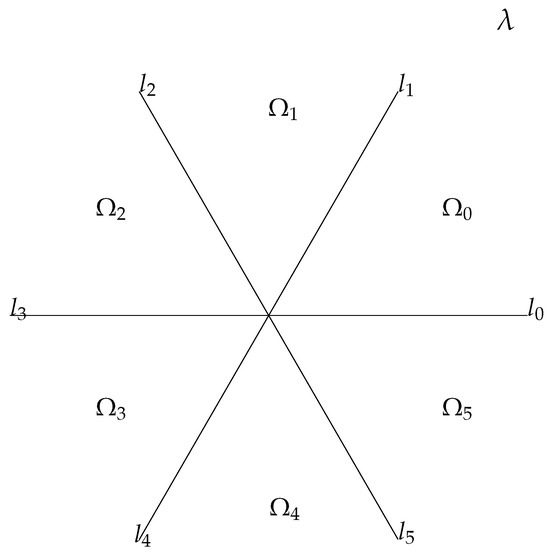Figure 1. The continuous spectrum of L fills the rays $l_k$, $k=0,\dots ,5$. The sectors of analyticity of ${\chi }_i(x,t,\lambda )$ are denoted by ${\Omega }_k$.

Solving (35) leads to the rays being defined by

$$\begin{array}{c}\hfill l_k:arg\lambda ={\displaystyle \frac{\pi k}{3}},k=0,\dots 5.\end{array}$$

(36)

2.

The regions of analyticity of the FASs are the sectors

$$\begin{array}{c}\hfill {\Omega }_k\equiv \left\{{\displaystyle \frac{k\pi }{3}}<arg\lambda <{\displaystyle \frac{(k+1)\pi }{3}}\right\}.\end{array}$$

(37)

3.

The FASs are analytic in the sectors ${\Omega }_k$ as follows:

$$\begin{array}{c}\hfill {\chi }_1:{\Omega }_0,{\Omega }_2,{\Omega }_4;\\ \hfill {\chi }_2:{\Omega }_1,{\Omega }_3,{\Omega }_5;\end{array}$$

(38)

We will abuse the notations when convenient and write ${\chi }_k$, where if $k>2$ then it is taken modulo 2.

4.

The scattering data is obtained by the limits of the FASs along both sides of the rays $l_k{e}^{\pm i0}$:

$$\begin{array}{cc}\hfill \underset{x\to \infty }{lim}{e}^{i{\lambda }^{3}Jx}{\chi }_1(x,t,\lambda )e^{-i{\lambda }^{3}Jx}& =S_1(t,\lambda )D_1^{+}\left(\lambda \right),\hfill \\ \hfill \underset{x\to -\infty }{lim}{e}^{i{\lambda }^{3}Jx}{\chi }_1(x,t,\lambda )e^{-i{\lambda }^{3}Jx}& =T_1(t,\lambda )D_1^{-}\left(\lambda \right),\hfill \end{array}\forall \lambda \in l_k{e}^{+i0},k=0,2,4$$

(39)

$$\begin{array}{cc}\hfill \underset{x\to \infty }{lim}{e}^{i{\lambda }^{3}Jx}{\chi }_2(x,t,\lambda )e^{-i{\lambda }^{3}Jx}& =S_2(t,\lambda )D_2^{+}\left(\lambda \right),\hfill \\ \hfill \underset{x\to -\infty }{lim}{e}^{i{\lambda }^{3}Jx}{\chi }_2(x,t,\lambda )e^{-i{\lambda }^{3}Jx}& =T_2(t,\lambda )D_2^{-}\left(\lambda \right),\hfill \end{array}\forall \lambda \in l_k{e}^{-i0},k=1,3,5$$

(40)

with

$$\begin{array}{cc}\hfill S_1(t,\lambda )& =\left(\begin{array}{cc}1& 0\\ {\rho }^{+}& 1\end{array}\right),S_2(t,\lambda )=\left(\begin{array}{cc}1& -{\rho }^{-}\\ 0& 1\end{array}\right),\hfill \\ \hfill T_1(t,\lambda )& =\left(\begin{array}{cc}1& {\tau }^{+}\\ 0& 1\end{array}\right),T_2\left(\lambda \right)=\left(\begin{array}{cc}1& 0\\ -{\tau }^{-}& 1\end{array}\right),\hfill \\ \hfill D_1^{+}(t,\lambda )& =\left(\begin{array}{cc}{a}^{+}& 0\\ 0& 1\end{array}\right),D_2^{+}\left(\lambda \right)=\left(\begin{array}{cc}1& 0\\ 0& a^{-}\end{array}\right),\hfill \\ \hfill D_1^{-}(t,\lambda )& =\left(\begin{array}{cc}1& 0\\ 0& a^{+}\end{array}\right),D_2^{-}\left(\lambda \right)=\left(\begin{array}{cc}{a}^{-}& 0\\ 0& 1\end{array}\right),\hfill \end{array}$$

(41)

where

$${\rho }^{\pm }={\displaystyle \frac{b^{\pm }}{a^{\pm }}},{\tau }^{\pm }={\displaystyle \frac{b^{\mp }}{a^{\pm }}},$$

(42)

are known as reflection coefficients. The scattering data satisfies

$$S_1{D}_1^{+}{\hat{D}}_1^{-}\widehat{T_1}=S_2{D}_2^{+}{\hat{D}}_2^{-}\widehat{T_2}=T(t,\lambda ),\lambda \in l_k.$$

(43)

Equation (43) is the Gauss decomposition of the scattering matrix $T(t,\lambda )$.

4.2. Riemann–Hilbert Problem with Canonical Normalization

The fundamental analytic solutions satisfy a (multiplicative) Riemann–Hilbert problem (RHP):

$$\begin{array}{cc}\hfill {\chi }_{k+1}(x,t,\lambda )& ={\chi }_k(x,t,\lambda )G_k(x,t,\lambda ),\lambda \in l_k,\hfill \\ \hfill G_k(x,t,\lambda )& =e^{-i{\lambda }^{3}Jx}{\widehat{D_k}}^{+}{\hat{S}}_k(t,\lambda )S_{k+1}{D}_{k+1}^{+}(t,\lambda )e^{i{\lambda }^{3}Jx}.\hfill \end{array}$$

(44)

The RHP is canonically normalized:

$$\underset{\lambda \to \infty }{lim}{\chi }_k(x,t,\lambda )=11.$$

(45)

The Zakharov–Shabat system can be generalized for Lax operators that are polynomial in the spectral parameter [30] to show that FASs are a solution of

$$i{\displaystyle \frac{\partial {\chi }_k}{\partial x}}+(U_0+\lambda U_1+{\lambda }^2{U}_2){\chi }_k(x,t,\lambda )-{\lambda }^3[J,{\chi }_k(x,t,\lambda )]=0.$$

(46)

Note that we can express the FASs in terms of the potentials. If ${\chi }_k(x,t,\lambda )$ is canonically normalized, it can be represented as

$$\begin{array}{c}\hfill {\chi }_k(x,t,\lambda )=exp\left(\mathcal{Q}(x,t,\lambda )\right),\end{array}$$

(47)

where

$$\begin{array}{c}\hfill \mathcal{Q}(x,t,\lambda )=\sum _{s=1}^{\infty }{\lambda }^{-s}{Q}_s(x,t).\end{array}$$

(48)

Only the first three terms need to be independent:

$$\mathcal{Q}(x,t,\lambda )={\displaystyle \frac{Q_1(x,t)}{\lambda }}+{\displaystyle \frac{Q_2(x,t)}{{\lambda }^2}}+{\displaystyle \frac{Q_3(x,t)}{{\lambda }^3}}+\dots$$

(49)

with higher terms expressed as functions of $Q_1(x,t),Q_2(x,t),Q_3(x,t)$ and their derivatives. Then, the potentials of L can be expressed as

$$\begin{array}{cc}\hfill U_2& ={\mathrm{ad}}_J{Q}_1,\hfill \\ \hfill U_1& ={\mathrm{ad}}_J{Q}_2-{\displaystyle \frac{1}{2}}{\mathrm{ad}}_{Q_1}^{2}J,\hfill \\ \hfill U_0& ={\mathrm{ad}}_J{Q}_3-{\displaystyle \frac{1}{2}}\left({\mathrm{ad}}_{Q_1}{\mathrm{ad}}_{Q_2}+{\mathrm{ad}}_{Q_2}{\mathrm{ad}}_{Q_1}\right)J-{\displaystyle \frac{1}{6}}{\mathrm{ad}}_{Q_1}^{3}J.\hfill \end{array}$$

(50)

To show that the the corresponding Reimman–Hilbert problem is canonically normalized, it is sufficient to show that $Q_1(x,t),Q_2(x,t),Q_3(x,t)$ can be expressed in terms of the potentials $U_0(x,t),U_1(x,t),U_2(x,t)$. Inverting (50) we have

$$\begin{array}{cc}\hfill & Q_1={\mathrm{ad}}_J^{-1}{U}_2,\hfill \\ \hfill & Q_2={\mathrm{ad}}_J^{-1}\left(U_1+{\displaystyle \frac{1}{2}}\left[U_2,{\mathrm{ad}}_J^{-1}{U}_2\right]\right),\hfill \\ \hfill & Q_3={\mathrm{ad}}_J^{-1}\left(U_0+{\displaystyle \frac{1}{2}}\left(\left({\mathrm{ad}}_{Q_1}{\mathrm{ad}}_{Q_2}+{\mathrm{ad}}_{Q_2}{\mathrm{ad}}_{Q_1}\right)J\right)+{\displaystyle \frac{1}{6}}{\mathrm{ad}}_{Q_1}^{3}J\right).\hfill \end{array}$$

(51)

We have mentioned that ${\chi }_k(x,t,\lambda )$ are not exactly the FASs of the Lax operator. To be precise, the FASs of L are in actuality

$${\zeta }_k(x,t,\lambda )={\chi }_k(x,t,\lambda )e^{-i{\lambda }^{3}Jx},$$

(52)

satisfying

$$L{\zeta }_k=i{\partial }_x{\zeta }_k+U(x,t,\lambda ){\zeta }_k-{\lambda }^{3}J{\zeta }_k=0.$$

(53)

4.3. Time Dependence of the Scattering Data

Consider one of the Jost solutions of L, say $\varphi$. In general we have that

$$L\varphi (x,t,\lambda )=0,M\varphi (x,t,\lambda )-\varphi (x,t,\lambda )\Gamma \left(\lambda \right)=0,$$

(54)

where $\Gamma \left(\lambda \right)$ is a constant matrix. The idea is to choose $\Gamma \left(\lambda \right)$ in such a way that the scattering data satisfy a linear evolution equation. Let us calculate the following limit:

$$\begin{array}{cc}\hfill & \underset{x\to -\infty }{lim}{e}^{i{\lambda }^{3}Jx}\left(M\varphi \right(x,t,\lambda )-\varphi (x,t,\lambda )\Gamma (\lambda \left)\right)=\hfill \\ \hfill & =\underset{x\to -\infty }{lim}{e}^{i{\lambda }^{3}Jx}\left[\left(i{\displaystyle \frac{\partial }{\partial t}}+\sum _{p=0}^4{\lambda }^p{V}_p-{\lambda }^{5}J\right)\varphi (x,t,\lambda )-\varphi (x,t,\lambda )\Gamma \left(\lambda \right)\right]\hfill \\ \hfill & =-{\lambda }^{5}J-\Gamma \left(\lambda \right)=0,\hfill \end{array}$$

(55)

where we have used the fact that ${lim}_{x\to \pm \infty }{V}_p(x,t)=0$. From (55) we obtain

$$\Gamma \left(\lambda \right)=-{\lambda }^{5}J.$$

(56)

We can derive the evolution for the Gauss factors of the scattering matrix. Assuming $\lambda \in l_k{e}^{i0}$, let us calculate the following limit:

$$\begin{array}{cc}\hfill & \underset{x\to \infty }{lim}{e}^{i{\lambda }^{3}Jx}\left(M{\zeta }_k(x,t,\lambda )-{\zeta }_k(x,t,\lambda )\Gamma \left(\lambda \right)\right)=\hfill \\ \hfill & =\underset{x\to \infty }{lim}{e}^{i{\lambda }^{3}Jx}\left[\left(i{\displaystyle \frac{\partial }{\partial t}}+\sum _{p=0}^4{\lambda }^p{V}_p-{\lambda }^{5}J\right){\zeta }_k(x,t,\lambda )-{\zeta }_k(x,t,\lambda )\Gamma \left(\lambda \right)\right]\hfill \\ \hfill & =i{\displaystyle \frac{\partial S_k{D}_k^{+}}{\partial t}}-{\lambda }^5\left[J,S_k{D}_k^{+}\right]=0,\lambda \in l_k.\hfill \end{array}$$

(57)

Splitting the above into diagonal and off-diagonal parts, we find that

$$\begin{array}{cc}\hfill i{\displaystyle \frac{\partial S_k}{\partial t}}-{\lambda }^5\left[J,S_k\right]& =0,\hfill \\ \hfill i{\displaystyle \frac{\partial }{\partial t}}{D}_k^{+}=0.\end{array}$$

(58)

A similar limit can be calculated for $x\to -\infty$:

$$\begin{array}{cc}\hfill & \underset{x\to -\infty }{lim}{e}^{i{\lambda }^{3}Jx}\left(M{\zeta }_k(x,t,\lambda )-{\zeta }_k(x,t,\lambda )\Gamma \left(\lambda \right)\right)=\hfill \\ \hfill & =\underset{x\to -\infty }{lim}{e}^{i{\lambda }^{3}Jx}\left[\left(i{\displaystyle \frac{\partial }{\partial t}}+\sum _{p=0}^4{\lambda }^p{V}_p-{\lambda }^{5}J\right){\zeta }_k(x,t,\lambda )-{\zeta }_k(x,t,\lambda )\Gamma \left(\lambda \right)\right]\hfill \\ \hfill & =i{\displaystyle \frac{\partial T_k{D}_k^{-}}{\partial t}}-{\lambda }^5[J,T_k{D}_k^{-}]=0,\lambda \in l_k.\hfill \end{array}$$

(59)

Again, considering diagonal and off-diagonal parts, we find

$$\begin{array}{cc}\hfill i{\displaystyle \frac{\partial T_k}{\partial t}}-{\lambda }^5\left[J,T_k\right]& =0,\hfill \\ \hfill i{\displaystyle \frac{\partial D_k^{-}}{\partial t}}=0.\end{array}$$

(60)

The solution of the above equations is given by (written component-wise)

$$S_{k,mn}(t,\lambda )=e^{-i{\lambda }^5(J_{mm}-J_{nn})t}{S}_{k,mn}(0,\lambda ),T_{k,mn}(t,\lambda )=e^{-i{\lambda }^5(J_{mm}-J_{nn})t}{T}_{k,mn}(0,\lambda ),$$

(61)

with the factors $D_k^{\pm }$ being time-independent. We can combine all of the above to derive the evolution for the scattering matrix

$$i{\displaystyle \frac{\partial T}{\partial t}}-{\lambda }^5[K,T]=0,$$

(62)

with a solution (written component-wise)

$$T_{mn}(t,\lambda )=e^{-i{\lambda }^5(J_{mm}-J_{nn})t}{T}_{mn}(0,\lambda ).$$

(63)

Solving the corresponding system of non-linear evolution equations (NLEEs) reduces to the following:

1.

Given Cauchy data $U(x,0,\lambda )$, using the equation for the FASs, i.e.,

$$i{\displaystyle \frac{\partial {\chi }_k}{\partial x}}+(U_0(x,0)+\lambda U_1(x,0)+{\lambda }^2{U}_2(x,0)){\chi }_k-{\lambda }^3[J,{\chi }_k]=0,$$

(64)

find ${\chi }_k(x,0,\lambda ),k=1,2$.

2.

Using Equations (39) and (40), find the Gauss factors for $t=0$ of the scattering matrix. Using them, reconstruct the scattering matrix $T(0,\lambda )$.

3.

Using (63) find $T(t,\lambda )$.

4.

Solve the inverse scattering problem for $T(t,\lambda )$ to find the time dependence of the potentials. This step is performed using the Gel’fand–Levitan–Marchenko (GLM) equation [48], which should be properly generalized for the L polynomial in $\lambda$. This is more involved and will be performed in a future work. Here, we will just note that the potentials can be recovered using the FASs ${\chi }_k(x,t,\lambda )$ by calculating the limit

$$\underset{\lambda \to \infty }{lim}\left(i{\displaystyle \frac{\partial {\chi }_k}{\partial x}}+(U_0+\lambda U_1+{\lambda }^2{U}_2){\chi }_k-{\lambda }^3[J,{\chi }_k]\right)=0.$$

(65)

5. Soliton-like Solutions

In what follows we will only consider the L operator. Note that there will be equivalent equations following from the M operator too. The main tool we will use is the dressing method [17,30,36]. The idea is to find $u(x,t,\lambda )\in SL(2,\mathbb{C})$ such that, starting from an already known solution ${\psi }_0(x,t,\lambda )$, i.e.,

$$\begin{array}{cc}\hfill & i{\partial }_x{\psi }_0+U_n(x,t,\lambda ){\psi }_0-{\lambda }^{3}J{\psi }_0=0,\hfill \\ \hfill & U_n(x,t,\lambda )=U_{n,0}(x,t)+\lambda U_{n,1}(x,t)+{\lambda }^2{U}_{n,2}(x,t),\hfill \end{array}$$

(66)

we have that the function

$$\psi (x,t,\lambda )=u(x,t,\lambda ){\psi }_0(x,t,\lambda )$$

(67)

is a solution of

$$\begin{array}{cc}\hfill & i{\partial }_x\psi +U_d(x,t,\lambda )\psi -{\lambda }^{3}J\psi =0,\hfill \\ \hfill & U_d(x,t,\lambda )=U_{d,0}(x,t)+\lambda U_{d,1}(x,t)+{\lambda }^2{U}_{d,2}(x,t).\hfill \end{array}$$

(68)

The matrix-valued function $u(x,t,\lambda )$ is called the dressing factor. We will call $U_n(x,t,\lambda )$ the naked potential and $U_d(x,t,\lambda )$ the dressed potential. We also require that $u(x,t,\lambda )$ be normalized, i.e.,

$$\underset{\lambda \to \infty }{lim}u(x,t,\lambda )=11.$$

(69)

The dressing factor must be compatible with the imposed reductions (14):

$$\begin{array}{c}\hfill Cu(x,t,-\lambda )C^{-1}=u(x,t,\lambda ),\end{array}$$

(70)

$$\begin{array}{c}\hfill u{(x,t,{\lambda }^{\ast })}^{†}=u^{-1}(x,t,\lambda ).\end{array}$$

(71)

By substituting (67) into (68), we can write the following equation for the dressing factor:

$$i{\partial }_{x}u-u{U}_n+U_{d}u-{\lambda }^3\left[J,u\right]=0.$$

(72)

Consider the normalization condition (69). If the dressing factor is analytic in the whole $\lambda$ plane and has no singularities, then by Liouville’s theorem it is a constant. Therefore, any nontrivial dressing factor must have singularities. We will consider the simplest case, i.e., the dressing factor has a simple pole at ${\lambda }_0$. This, along with the reduction condition (70), fixes the dressing factor to have the form

$$u(x,t,\lambda )=11+{\displaystyle \frac{A}{\lambda -{\lambda }_0}}-{\displaystyle \frac{CA{C}^{-1}}{\lambda +{\lambda }_0}}.$$

(73)

The dressing factor must also satisfy (71), which means that

$$u^{-1}(x,t,\lambda )u(x,t,\lambda )=u{(x,t,{\lambda }^{\ast })}^{†}u(x,t,\lambda )=11.$$

(74)

By calculating the residue of (74) at $\lambda \to {\lambda }_0$, we get

$$A\left(11+{\displaystyle \frac{A^{†}}{{\lambda }_0-{\lambda }_0^{\ast }}}-{\displaystyle \frac{C{A}^{†}{C}^{-1}}{{\lambda }_0+{\lambda }_0^{\ast }}}\right)=0.$$

(75)

In order to find a nontrivial solution to the above, consider

$$A=|m⟩⟨n|.$$

(76)

The vectors $|m⟩,|n⟩$ are called polarization vectors. By substituting (76) into the residue at $\lambda \to {\lambda }_0$ of (72), we get

$$\begin{array}{cc}\hfill & \left(i{\partial }_x|m⟩+U_d(x,t,{\lambda }_0)|m⟩-{\lambda }_0^{3}J|m⟩\right)⟨n|\hfill \\ \hfill & +|m⟩\left(i{\partial }_x⟨n|-⟨n|U_n(x,t,{\lambda }_0)+{\lambda }_0^3⟨n|J\right)=0,\hfill \end{array}$$

(77)

which implies that

$$\begin{array}{cc}& i{\partial }_x|m⟩+U_d(x,t,{\lambda }_0)|m⟩-{\lambda }_0^{3}J|m⟩=0,\end{array}$$

(78)

$$\begin{array}{cc}& i{\partial }_x|n⟩+U_n(x,t,{\lambda }_0^{\ast })|n⟩-{\lambda }_0^{\ast 3}J|n⟩=0,\end{array}$$

(79)

i.e., $|m⟩$ satisfies the equation with the dressed potential $U_d(x,t,{\lambda }_0)$, while $|n⟩$ is a solution with the naked potential $U_n(x,t,{\lambda }_0^{\ast })$. Note that while $i{\partial }_x$ is self-adjoint with respect to the usual $L^2$ inner product, it is not invariant under matrix Hermitian conjugation. Now, note that $|m⟩$ can be expressed as a linear function of $|n⟩$. Considering (76), from (75) we get

$$⟨n|\left(11+{\displaystyle \frac{|n⟩⟨m|}{{\lambda }_0-{\lambda }_0^{\ast }}}-{\displaystyle \frac{C|n⟩⟨m|C^{-1}}{{\lambda }_0+{\lambda }_0^{\ast }}}\right)=0,$$

(80)

and by taking the Hermitian conjugate (and using the fact that $C^{†}=C^{-1}=-C$), expanding the bracket, and rearranging the terms we get

$$\left(11{\displaystyle \frac{⟨n,n⟩}{{\lambda }_0-{\lambda }_0^{\ast }}}-{\displaystyle \frac{⟨n,Cn⟩C}{{\lambda }_0+{\lambda }_0^{\ast }}}\right)|m⟩=B|m⟩=|n⟩.$$

(81)

The explicit form of B is

$$B=\left(\begin{array}{cc}{\displaystyle \frac{{n_1}^{\ast }{n}_1+{n_2}^{\ast }{n}_2}{{\lambda }_0-{{\lambda }_0}^{\ast }}}& {\displaystyle \frac{{n_2}^{\ast }{n}_1-{n_1}^{\ast }{n}_2}{{\lambda }_0+{{\lambda }_0}^{\ast }}}\\ -{\displaystyle \frac{{n_2}^{\ast }{n}_1-{n_1}^{\ast }{n}_2}{{\lambda }_0+{{\lambda }_0}^{\ast }}}& {\displaystyle \frac{{n_1}^{\ast }{n}_1+{n_2}^{\ast }{n}_2}{{\lambda }_0-{{\lambda }_0}^{\ast }}}\end{array}\right).$$

(82)

This can easily be inverted (where $\left|B\right|$ is the determinant of a matrix B):

$$B^{-1}={\displaystyle \frac{1}{\left|B\right|}}\left(\begin{array}{cc}{B}_{22}& -B_{12}\\ -B_{21}& B_{11}\end{array}\right),$$

(83)

which means that

$$|m⟩=B^{-1}|n⟩.$$

(84)

Written explicitly, this reads as

$$m_1={\displaystyle \frac{N_1}{D}},m_2={\displaystyle \frac{N_2}{D}},$$

(85)

where

$$\begin{array}{cc}\hfill N_1& =({\lambda }_0^2-{\lambda }_0^{\ast 2})\left(\left((n_1^2-n_2^2)n_1^{\ast }+2n_1{n}_2{n}_2^{\ast }\right){\lambda }_0^{\ast }+{\lambda }_0{n}_1^{\ast }(n_1^2+n_2^2)\right),\hfill \\ \hfill N_2& =({\lambda }_0^2-{\lambda }_0^{\ast 2})\left(\left((n_2^2-n_1^2)n_2^{\ast }+2n_1{n}_1^{\ast }{n}_2\right){\lambda }_0^{\ast }+{\lambda }_0{n}_2^{\ast }(n_1^2+n_2^2)\right),\hfill \\ \hfill D& =(n_1^{\ast 2}+n_2^{\ast 2})(n_1^2+n_2^2)[{\left({\lambda }_0^{\ast }\right)}^2+{\lambda }_0^2]\hfill \\ \hfill & +2{\lambda }_0{\lambda }_0^{\ast }\left((n_1-n_2)n_1^{\ast }+n_2^{\ast }(n_1+n_2)\right)\left((n_1+n_2)n_1^{\ast }-n_2^{\ast }(n_1-n_2)\right).\hfill \end{array}$$

(86)

From (72) we can express the potentials in terms of the residue of the dressing factor. By factoring ${\displaystyle \frac{1}{{\lambda }^2-{\lambda }_0^2}}$ as a common denominator and taking the limit $\lambda \to \infty$ in (72), we get

$$\begin{array}{cc}\hfill U_{d,2}& =U_{n,2}+\left[J,A-CA{C}^{-1}\right],\hfill \\ \hfill U_{d,1}& =U_{n,1}+{\lambda }_0\left[J,A+CA{C}^{-1}\right]-U_{d,2}\left(A-CA{C}^{-1}\right)+\left(A-CA{C}^{-1}\right)U_{n,2},\hfill \\ \hfill U_{d,0}& =U_{n,0}-{\lambda }_0\left(U_{d,2}\left(A+CA{C}^{-1}\right)-\left(A+CA{C}^{-1}\right)U_{n,2}\right)+{\lambda }_0^2\left(U_{d,2}-U_{n,2}\right)\hfill \\ \hfill & -\left(U_{d,1}\left(A-CA{C}^{-1}\right)-\left(A-CA{C}^{-1}\right)U_{n,1}\right).\hfill \end{array}$$

(87)

One-Soliton Solutions

When we say one-soliton solutions, we mean one soliton-like solution in each component. This corresponds to a dressing factor having simple poles at ${\lambda }_0,-{\lambda }_0$. In this case $U_n=0$. Then (79) implies that

$$i{\partial }_x|n⟩-{\lambda }_0^{\ast 3}J|n⟩=0.$$

(88)

Note that we have an analogous equation following from the M operator,

$$i{\partial }_t|n⟩-{\lambda }_0^{\mathrm{*5}}J|n⟩=0.$$

(89)

The above two equations can be easily solved to yield

$$|n⟩=e^{i{\lambda }_0^{\ast 3}Jx+i{\lambda }_0^{\ast 5}Jt}|n_0⟩,$$

(90)

where

$$|n_0⟩=\left(\begin{array}{c}{n}_{01}\\ n_{02}\end{array}\right)$$

(91)

is an arbitrary constant complex-valued vector. Explicitly this reads

$$\begin{array}{cc}\hfill n_1& =e^{i({\lambda }_0^{\ast 3}x+{\lambda }_0^{\ast 5}t)}{n}_{01},\hfill \\ \hfill n_2& =e^{-i({\lambda }_0^{\ast 3}x+{\lambda }_0^{\ast 5}t)}{n}_{02}.\hfill \end{array}$$

(92)

The one-soliton solution is described by three complex parameters—$n_{01},n_{02},{\lambda }_0$. From (87) we can recover the potentials. Let ${\lambda }_0=\mu +i\nu$ and

$$\begin{array}{cc}\hfill F_1& =n_1{n}_1^{\ast }+n_2{n}_2^{\ast },F_2=n_2{n}_1^{\ast }+n_1{n}_2^{\ast },\hfill \\ \hfill F_3& =n_1{n}_1^{\ast }-n_2{n}_2^{\ast },F_4=n_1{n}_2^{\ast }-n_2{n}_1^{\ast }.\hfill \end{array}$$

(93)

Then we can write the potentials as

$$\begin{array}{cc}\hfill q_1& =-4\nu \mu {\displaystyle \frac{\left(F_2{F}_1{\mu }^3+3i{F}_4{\mu }^2\nu F_3-3F_2{F}_1{\nu }^2\mu -i{F}_4{\nu }^3{F}_3\right)}{F_1^2{\mu }^2-F_4^2{\nu }^2}},\hfill \\ \hfill q_2& =4\nu \mu {\displaystyle \frac{\left(i{F}_1^3{F}_4{\mu }^4-2F_3{F}_2{F}_1^2\nu {\mu }^3+i(2F_2^2-2F_3^2-F_4^2+F_1^2)F_4{F}_1{\nu }^2{\mu }^2-2F_3{F}_2{F}_4^2{\nu }^3\mu -i{\nu }^4{F}_1{F}_4^3\right)}{{(F_1^2{\mu }^2-F_4^2{\nu }^2)}^2}},\hfill \\ \hfill q_3& =-4\nu \mu {\displaystyle \frac{\left(F_2{F}_1\mu +i{F}_3{F}_4\nu \right)}{F_1^2{\mu }^2-F_4^2{\nu }^2}}.\hfill \end{array}$$

(94)

The explicit form of $F_i$ is given by

$$\begin{array}{cc}\hfill F_1& =\left(|n_{01}{|}^2+{|n_{02}|}^2\right)cosh\left((2{\nu }^5-20{\nu }^3{\mu }^2+10\nu {\mu }^4)t-2x{\nu }^3+6x{\mu }^2\nu \right)\hfill \\ \hfill & +\left(|n_{01}{|}^2-{\left|n_{02}\right|}^2\right)sinh\left((2{\nu }^5-20{\nu }^3{\mu }^2+10\nu {\mu }^4)t-2x{\nu }^3+6x{\mu }^2\nu \right),\hfill \\ \hfill F_2& =\left(n_{02}{n}_{01}^{\ast }+n_{01}{n}_{02}^{\ast }\right)cos\left(2\mu \left(({\mu }^4-10{\nu }^2{\mu }^2+5{\nu }^4)t+x({\mu }^2-3{\nu }^2)\right)\right)\hfill \\ \hfill & +i\left(n_{01}{n}_{02}^{\ast }-n_{02}{n}_{01}^{\ast }\right)sin\left(2\mu \left(({\mu }^4-10{\nu }^2{\mu }^2+5{\nu }^4)t+x({\mu }^2-3{\nu }^2)\right)\right),\hfill \\ \hfill F_3& =\left(|n_{01}{|}^2-{\left|n_{02}\right|}^2\right)cosh\left((2{\nu }^5-20{\nu }^3{\mu }^2+10\nu {\mu }^4)t-2x{\nu }^3+6x{\mu }^2\nu \right)\hfill \\ \hfill & +\left(|n_{01}{|}^2+{\left|n_{02}\right|}^2\right)sinh\left((2{\nu }^5-20{\nu }^3{\mu }^2+10\nu {\mu }^4)t-2x{\nu }^3+6x{\mu }^2\nu \right),\hfill \\ \hfill F_4& =\left(n_{01}{n}_{02}^{\ast }-n_{02}{n}_{01}^{\ast }\right)cos\left(2\mu \left(({\mu }^4-10{\nu }^2{\mu }^2+5{\nu }^4)t+x({\mu }^2-3{\nu }^2)\right)\right)\hfill \\ \hfill & +i\left(n_{01}{n}_{02}^{\ast }+n_{02}{n}_{01}^{\ast }\right)sin\left(2\mu \left(({\mu }^4-10{\nu }^2{\mu }^2+5{\nu }^4)t+x({\mu }^2-3{\nu }^2)\right)\right).\hfill \end{array}$$

(95)

The expressions for the potentials $q_i$ are quite cumbersome, which significantly complicates the general analysis of the solution. We can classify the solutions into at least three classes:

• Breather solutions. In general, the solution is a breather solution (with all components traveling together), provided that the pole ${\lambda }_0$ does not lie on the continuous spectrum (see Figure 1). For example, let $n_{01}=1,n_{02}=1,{\lambda }_0=1+i$. Then the solution is given by

  $$\begin{array}{cc}\hfill q_1& =16{\displaystyle \frac{cos(4x+8t)cosh(4x-8t)-sin(4x+8t)sinh(4x-8t)}{2-cos(8x+16t)+cosh(8x-16t)}},\hfill \\ \hfill q_2& =-{\displaystyle \frac{8}{{\left(2-cos(8x+16t)+cosh(8x-16t)\right)}^2}}\hfill \\ \hfill & \times (8sin(4x+8t)cosh(4x-8t)-cos(12x+24t)sinh(4x-8t)\hfill \\ \hfill & -cos(4x+8t)sinh(12x-24t)),\hfill \\ \hfill q_3& =-8{\displaystyle \frac{\left(cos(4x+8t)cosh(4x-8t)+sin(4x+8t)sinh(4x-8t)\right)}{2-cos(8x+16t)+cosh(8x-16t)}}.\hfill \end{array}$$

  (96)
  Plots of the solution can be found in Figure 2 and Figure 3.
  

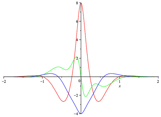  Figure 2. One-pole solution at $t=0$ for $x\in [-2,2]$ with parameters $n_{01}=1,n_{02}=1,{\lambda }_0=(1+i)$. The components are colored as follows: $q_1$—red; $q_2$—green; and $q_3$—blue.
  

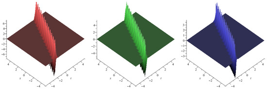  Figure 3. Spatio-temporal evolution of the solution for $t\in [-5,5],x\in [-5,5].$.
• Rogue waves. If ${\lambda }_0=e^{{\displaystyle \frac{ik\pi }{3}}},k\in \{1,2,4,5\},$ we obtain a rouge wave—a temporally localized solution that starts from 0 for all components at $t\to -\infty$, is non-zero and peaks at $t=0$, and then goes to 0 again for $t\to \infty$. Note, that while the solution is temporally localized, it is not spatially confined. As an example, let $n_{01}=1,n_{02}=1,{\lambda }_0=e^{{\displaystyle \frac{i\pi }{3}}}={\displaystyle \frac{1}{2}}+i{\displaystyle \frac{\sqrt{3}}{2}}$. Explicitly we have

  $$\begin{array}{cc}\hfill q_1& ={\displaystyle \frac{8cos(2x-t)\sqrt{3}cosh\left(t\sqrt{3}\right)}{4-3cos(2t-4x)+cosh\left(2t\sqrt{3}\right)}},\hfill \\ \hfill q_2& ={\displaystyle \frac{2}{{\left(4-3cos(2t-4x)+cosh\left(2t\sqrt{3}\right)\right)}^2}}\hfill \\ \hfill & \times (3cos(2x-t)\left(2sinh\left(t\sqrt{3}\right)-sinh\left(3t\sqrt{3}\right)\right)\hfill \\ \hfill & -9cos(6x-3t)sinh\left(t\sqrt{3}\right)+3sin(6x-3t)\sqrt{3}cosh\left(t\sqrt{3}\right)\hfill \\ \hfill & -\sqrt{3}sin(2x-t)\left(30cosh\left(t\sqrt{3}\right)-cosh\left(3t\sqrt{3}\right)\right)),\hfill \\ \hfill q_3& =4{\displaystyle \frac{3sin(2x-t)sinh\left(t\sqrt{3}\right)-cos(2x-t)\sqrt{3}cosh\left(t\sqrt{3}\right)}{4-3cos(4x-2t)+cosh\left(2t\sqrt{3}\right)}}.\hfill \end{array}$$

  (97)
  Plots of the solution can be found in Figure 4 and Figure 5.
  

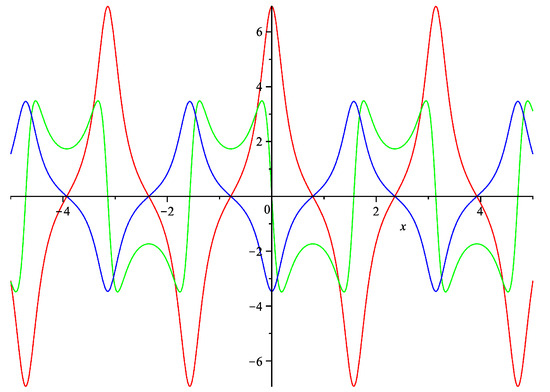  Figure 4. One-pole solution at $t=0$ for $x\in [-5,5]$ with parameters $n_{01}=1,n_{02}=1,{\lambda }_0=e^{{\displaystyle \frac{i\pi }{3}}}$. The components are colored as follows: $q_1$—red; $q_2$—green; and $q_3$—blue.
  

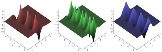  Figure 5. Spatio-temporal evolution of the solution for $t\in [-5,5],x\in [-5,5].$.
• Plane wave-like solutions. As the pole ${\lambda }_0$ approaches the real axis, the solution approaches a plane wave, with the amplitude quickly tending to zero. Figure 6 and Figure 7 contain plots of the solution for $n_{01}=1,n_{02}=1,{\lambda }_0=1+i{10}^{-2}$.
  

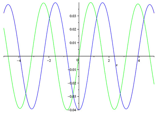  Figure 6. The solution at $t=0$ for $x\in [-5,5]$ with parameters $n_{01}=1,n_{02}=1,{\lambda }_0=1+i{10}^{-2}$. The components are colored as follows: $q_1$—red; $q_2$—green; and $q_3$—blue. Here $q_1$ and $q_3$ are overlapping.
  

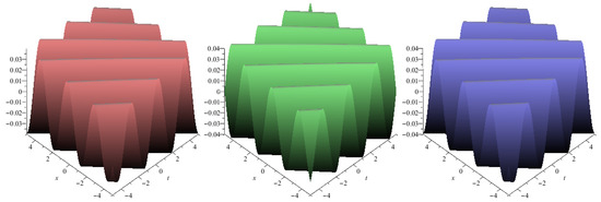  Figure 7. Spatio-temporal evolution of the solution for $t\in [-5,5],x\in [-5,5].$.

6. Conclusions and Discussion

Usually research on integrable models is motivated by one of two interests. For a pure mathematician, the subject is interesting without considering the area of application of the model in question. Solving non-linear PDEs is challenging and has merit on its own. The other side is practical application. Modeling complex phenomena in physics usually leads to a system of NLEEs and sometimes (usually with the correct approximation) the equations are integrable. The truth is that only a fraction of all derived exactly solvable NLEEs have real practical application. This does not mean that new systems should not be studied, even if their practical application is yet unknown. In fact, probably the best strategy is to try and compile a list of all possible exactly solvable models, at least for a practical number of components. Such a list is almost exhausted for Lax operators linear in the spectral parameter, at least in $1+1$ dimensions. A natural direction, then, is to consider polynomial dependence on the spectral parameter.

While this paper formulates the basic scattering problem, it is far from complete. An extremely important point that is missing is solving the inverse scattering problem. Usually this is performed using the Gelfand–Levitan–Marchenko equation. It can be generalized to our case, but this is rather involved and is to be performed in a future work.

Another direction of future research is the Hamiltonian formulation of the NLEEs. Note that the scattering factors $D_k^{\pm }$ are time-independent; hence they can be used to generate integrals of motion. Any of those integrals can in principle be used as a Hamiltonian, provided we find the correct Poisson bracket. This can be performed if we find what is known as recursion operators of the L operator.

There is a hierarchy of equations related to the used L operator. Each member of this hierarchy is associated with an M operator of order (in the spectral parameter) $n=2k+1,k=2,3,4\dots$. This can also be performed by using recursion operators.

With all that said, it is our believe that the derived system of NLEEs will be of use in practice, for example in the fields of fluid dynamics, optics, and plasma physics.

References

- Drinfeld, V.; Sokolov, V. Equations of KdV type and simple Lie algebras. Sov. Math. Dokl. 1981, 23, 457–462. [Google Scholar]
- Drinfeld, V.; Sokolov, V. Lie algebras and equations of Korteweg-de Vries type. Sov. J. Math. 1985, 30, 1975–2036. [Google Scholar] [CrossRef]
- Gerdjikov, V.; Mladenov, D.; Stefanov, A.; Varbev, S. Integrable equations and recursion operators related to the affine Lie algebras Ar(1). J. Math. Phys. 2015, 56, 052702. [Google Scholar] [CrossRef]
- Gerdjikov, V.; Mladenov, D.; Stefanov, A.; Varbev, S. The mKdV-type equations related to Kac-Moody algebras. Theor. Math. Phys. 2021, 207, 604–625. [Google Scholar] [CrossRef]
- Gerdjikov, V.S.; Stefanov, A.A.; Iliev, I.D.; Boyadjiev, G.P.; Smirnov, A.O.; Matveev, V.B.; Pavlov, M.V. Recursion operators and hierarchies of mKdV equations related to the Kac-Moody algebras , and . Theor. Math. Phys. 2020, 204, 1110–1129. [Google Scholar] [CrossRef]
- Fordy, A.; Kulish, P. Nonlinear Schrödinger equations and simple Lie algebras. Commun. Math. Phys. 1983, 89, 427–443. [Google Scholar] [CrossRef]
- Gerdjikov, V. On spectral theory of Lax operators on symmetric spaces: Vanishing versus constant boundary conditions. J. Geom. Symmetry Phys. 2009, 15, 1–41. [Google Scholar]
- Gerdjikov, V.; Grahovski, G.; Kostov, N. Multicomponent equations of the nonlinear Schrödinger type on symmetric spaces and their reductions. Theoret. Math. Phys. 2005, 144, 1147–1156. [Google Scholar] [CrossRef]
- Manakov, S. On the theory of two-dimensional stationary self-focusing of electromagnetic waves. Sov. Phys. JETP 1974, 38, 248–253. [Google Scholar]
- Gerdjikov, V.; Kostov, N.; Valchev, T. Solutions of multi-component NLS models and Spinor Bose-Einstein condensates. Phys. D Nonlinear Phenom. 2009, 238, 1306–1310. [Google Scholar] [CrossRef]
- Athorne, C.; Fordy, A. Generalised KdV and MKdV equations associated with symmetric spaces. J. Phys. A Math. Gen. 1987, 20, 1377. [Google Scholar] [CrossRef]
- Zakharov, V.E.; Manakov, S.V. On the theory of resonance interactions of wave packets in nonlinear media. Zh. Exp. Teor. Fiz. 1975, 69, 1654–1673. [Google Scholar]
- Huang, G.X. Exact solitary wave solutions of three-wave interaction equations with dispersion. J. Phys. A Math. Gen. 2000, 33, 8477–8482. [Google Scholar] [CrossRef]
- Valiulis, G.; Staliunas, K. On integrability and soliton solutions of three-wave interaction equations. Lith. Phys. J. 1991, 31, 38–44. [Google Scholar]
- Degasperis, A.; Lombardo, S. Exact solutions of the 3-wave resonant interaction equation. Phys. D Nonlinear Phenom. 2006, 214, 157–168. [Google Scholar] [CrossRef][Green Version]
- Zakharov, V.; Shabat, A. Integration of nonlinear equations of mathematical physics by the method of inverse scattering. I. Funct. Anal. Appl. 1974, 8, 226–235. [Google Scholar] [CrossRef]
- Zakharov, V.; Shabat, A. Integration of nonlinear equations of mathematical physics by the method of inverse scattering. II. Funct. Anal. Appl. 1979, 13, 166–174. [Google Scholar] [CrossRef]
- Caudrey, P.J. The Inverse Problem for a General N × N Spectral Equation. Phys. D Nonlinear Phenom. 1982, 6, 51–56. [Google Scholar] [CrossRef]
- Beals, R.; Coifman, R.R. Scattering and Inverse Scattering for First Order Systems. Commun. Pure Appl. Math. 1984, 37, 39–90. [Google Scholar] [CrossRef]
- Beals, R.; Coifman, R.R. Inverse Scattering and Evolution Equations. Commun. Pure Appl. Math. 1985, 38, 29–42. [Google Scholar] [CrossRef]
- Beals, R.; Coifman, R.R. Scattering and Inverse Scattering for First Order Systems II. Inverse Probl. 1987, 3, 577–593. [Google Scholar] [CrossRef]
- Ma, W. Novel integrable Hamiltonian hierarchies with six potentials. Acta Math. Sci. 2024, 44, 2498–2508. [Google Scholar] [CrossRef]
- Zhang, S.; Li, H.; Xu, B. Inverse Scattering Integrability and Fractional Soliton Solutions of a Variable-Coefficient Fractional-Order KdV-Type Equation. Fractal Fract. 2024, 8, 520. [Google Scholar] [CrossRef]
- Zhan, S.; Wang, X.; Xu, B. Riemann-Hilbert Method Equipped with Mixed Spectrum for N-Soliton Solutions of New Three-Component Coupled Time-Varying Coefficient Complex mKdV Equations. Fractal Fract. 2024, 8, 355. [Google Scholar] [CrossRef]
- Alhejaili, S.H.; Alharbi, A. Structure of Analytical and Numerical Wave Solutions for the Nonlinear (1 + 1)-Coupled Drinfel’d-Sokolov-Wilson System Arising in Shallow Water Waves. Mathematics 2023, 11, 4598. [Google Scholar] [CrossRef]
- Kaup, D.; Newell, A. An exact solution for a derivative nonlinear Schrödinger equation. J. Math. Phys. 1978, 19, 798–801. [Google Scholar] [CrossRef]
- Chen, H.; Lee, Y.; Liu, C. Integrability of Nonlinear Hamiltonian Systems by Inverse Scattering Method. Phys. Scr. 1979, 20, 490. [Google Scholar] [CrossRef]
- Antonowicz, M.; Fordy, A.P. Factorisation of energy dependent Schrödinger operators: Miura maps and modified systems. Commun. Math. Phys. 1989, 124, 465–486. [Google Scholar] [CrossRef]
- Antonowicz, M.; Fordy, A.; Liu, Q. Energy-dependent third-order Lax operators. Nonlinearity 1991, 4, 669. [Google Scholar] [CrossRef]
- Gerdjikov, V.; Stefanov, A. Riemann-Hilbert problems, polynomial Lax pairs, integrable equations and their soliton solutions. Symmetry 2023, 15, 1933. [Google Scholar] [CrossRef]
- Shabat, A.B. A one-dimensional scattering theory. I. Differ. Uravn. 1972, 8, 164–178. [Google Scholar]
- Shabat, A.B. The inverse scattering problem for a system of differential equations. Funkts. Anal. Prilozhen. 1975, 9, 75–78. [Google Scholar] [CrossRef]
- Gerdjikov, V.; Yanovski, A. Riemann-Hilbert Problems, families of commuting operators and soliton equations. J. Phys. Conf. Ser. 2014, 482, 012017. [Google Scholar] [CrossRef]
- Zakharov, V.E.; Manakov, S.V. Construction of higher-dimensional nonlinear integrable systems and of their solutions. Funct. Anal. Its Appl. 1985, 19, 89–101. [Google Scholar] [CrossRef]
- Shepelsky, D. Riemann-Hilbert Methods in Integrable Systems. In Encyclopedia of Mathematical Physics; Elsevier: Amsterdam, The Netherlands, 2006; pp. 76–82. [Google Scholar] [CrossRef]
- Ivanov, R. On the dressing method for the generalised Zakharov-Shabat system. Nucl. Phys. B 2004, 694, 509–524. [Google Scholar] [CrossRef]
- Yang, J. Nonlinear Waves in Integrable and Nonintegrable Systems; SIAM: Philadelphia, PA, USA, 2010. [Google Scholar] [CrossRef]
- Lax, P.D. Integrals of nonlinear equations of evolution and solitary waves. Commun. Pure Appl. Math. 1968, 21, 467–490. [Google Scholar] [CrossRef]
- Krishnaswami, G.; Vishnu, T. An introduction to Lax pairs and the zero curvature representation. arXiv 2020, arXiv:2004.05791v1. [Google Scholar]
- Dunajski, M. Solitons, Instantons, and Twistors; Oxford Graduate Texts in Mathematics; Oxford University Press: Oxford, UK, 2024. [Google Scholar]
- Calogero, F. Integrable Systems: Overview. In Encyclopedia of Mathematical Physics; Françoise, J.P., Naber, G.L., Tsun, T.S., Eds.; Academic Press: Oxford, UK, 2006; pp. 106–123. [Google Scholar] [CrossRef]
- Fokas, A. Integrable Systems and the Inverse Scattering Method. In Encyclopedia of Mathematical Physics; Françoise, J., Naber, G., Tsun, T., Eds.; Academic Press: Oxford, UK, 2006; pp. 93–101. [Google Scholar] [CrossRef]
- Wadati, M. Introduction to solitons. Pramana 2001, 57, 841–847. [Google Scholar] [CrossRef]
- Carter, R. Lie Algebras of Finite and Affine Type; Cambridge University Press: Cambridge, UK, 2005. [Google Scholar]
- Helgason, S. Differential Geometry, Lie Groups and Symmetric Spaces; Graduate Studies in Mathematics; American Mathematical Society: Providence, RI, USA, 2012; Volume 34. [Google Scholar]
- Kac, V. Infinite Dimensional Lie Algebras; Cambridge University Press: Cambridge, UK, 1995. [Google Scholar]
- Mikhailov, A.V. The reduction problem and the inverse scattering problem. Phys. D 1981, 3, 73–117. [Google Scholar] [CrossRef]
- Gerdjikov, V.; Vilasi, G.; Yanovski, A. Integrable Hamiltonian Hierarchies: Spectral and Geometric Methods; Lecture Notes in Physics; Springer: Berlin/Heidelberg, Germany, 2008; Volume 748. [Google Scholar]
Disclaimer/Publisher’s Note: The statements, opinions and data contained in all publications are solely those of the individual author(s) and contributor(s) and not of MDPI and/or the editor(s). MDPI and/or the editor(s) disclaim responsibility for any injury to people or property resulting from any ideas, methods, instructions or products referred to in the content. |
© 2025 by the authors. Licensee MDPI, Basel, Switzerland. This article is an open access article distributed under the terms and conditions of the Creative Commons Attribution (CC BY) license (https://creativecommons.org/licenses/by/4.0/).