Article

Forecasting COVID-19 Cases, Hospital Admissions, and Deaths Based on Wastewater SARS-CoV-2 Surveillance Using Gaussian Copula Time Series Marginal Regression Model

1
School of Community and Environmental Health, College of Health Sciences, Old Dominion University, Norfolk, VA 23529, USA
2
Department of Mathematics & Statistics, College of Sciences, Old Dominion University, Norfolk, VA 23529, USA
3
Chesapeake Health Department, Chesapeake, VA 23320, USA
4
Division of Water and Wastewater, Virginia Department of Health, Richmond, VA 23219, USA
5
Technical Services Division, Hampton Road Sanitation District, Virginia Beach, VA 23455, USA
6
Public Utilities, City of Chesapeake, VA 23322, USA
*
Author to whom correspondence should be addressed.
COVID 2025, 5(2), 25; https://doi.org/10.3390/covid5020025
Submission received: 11 September 2024 / Revised: 6 February 2025 / Accepted: 14 February 2025 / Published: 18 February 2025
(This article belongs to the Section COVID Clinical Manifestations and Management)

Abstract

:
Modeling efforts are needed to predict trends in COVID-19 cases and related health outcomes, aiding in the development of management strategies and adaptation measures. This study was conducted to assess whether the SARS-CoV-2 viral load in wastewater could serve as a predictor for forecasting COVID-19 cases, hospitalizations, and deaths using copula-based time series modeling. SARS-CoV-2 RNA load in wastewater in Chesapeake, VA, was measured using the RT-qPCR method. A Gaussian copula time series (CTS) marginal regression model, incorporating an autoregressive moving average model and Gaussian copula function, was used as a forecasting model. Wastewater SARS-CoV-2 viral loads were correlated with COVID-19 cases. The forecasted model with both Poisson and negative binomial marginal distributions yielded trends in COVID-19 cases that closely paralleled the reported cases, with 90% of the forecasted COVID-19 cases falling within the 99% confidence interval of the reported data. However, the model did not effectively forecast the trends and the rising cases of hospital admissions and deaths. The forecasting model was validated for predicting clinical cases and trends with a non-normal distribution in a time series manner. Additionally, the model showed potential for using wastewater SARS-CoV-2 viral load as a predictor for forecasting COVID-19 cases.

1. Introduction

The emergence of SARS-CoV-2 has led to the global spread of COVID-19, resulting in devastating impacts. As of September 2022, the disease has caused over 6.4 million deaths worldwide. Vaccinations have played a crucial role in managing the pandemic, but the ongoing evolution of new virus mutations suggests that the virus is unlikely to be eradicated in the near future. Consequently, modeling efforts aimed at predicting COVID-19 trends are essential for developing effective management strategies and adaptation measures to address the challenges posed by the pandemic.
Wastewater-based surveillance has been considered as a tool to monitor and track SARS-CoV-2 RNA within communities in many countries [1,2]. The rationale for this includes several factors. First, wastewater-based surveillance can detect RNA from both nonviable and viable SARS-CoV-2 in both symptomatic and asymptomatic individuals [3,4,5]. Second, over 80% of the population lives in areas with wastewater treatment facilities. Third, well-established molecular analyses are available for detecting SARS-CoV-2 in wastewater [2]. Fourth, wastewater-based analysis offers higher positive detection rates than rectal and sputum swabs. Fifth, wastewater-based analysis is more efficient as it reduces the number of tests required to evaluate a large population. Also, it does not require patient consent and makes test results available earlier. Increasing studies on the relationships between wastewater SARS-CoV-2 RNA and the dynamics of the COVID-19 pandemic will allow researchers to better understand the application of wastewater-based surveillance in the COVID-19 pandemic [6,7].
SARS-CoV-2 RNA was detected in wastewater samples, with associations between trends in viral load in wastewater and community and clinical cases [1,6,7,8,9]. A time lag of 5 to 15 days was observed between SARS-CoV-2 viral load in wastewater and clinically diagnosed COVID-19 cases [10,11,12]. Increasing literature has shown that SARS-CoV-2 in wastewater serves as a useful predictor for forecasting COVID-19 cases [9,12,13,14]. However, limited or no studies have investigated whether wastewater SARS-CoV-2 viral load can reliably predict death cases and hospital admissions [15,16].
This study aimed to determine whether the newly developed copula time series (CTS) model could forecast COVID-19 cases, hospital admissions, and death cases using SARS-CoV-2 viral load in wastewater. A copula is a function that joins a multivariate distribution function to its one-dimensional marginal distribution functions [17]. The CTS model integrated an autoregressive moving average (ARMA) model and Gaussian copula function [9]. With the ARMA model, the CTS model analyzed time series data, while the copula functions equip the CTS model with several strengths, including (1) handling multiple continuous and/or noncontinuous variables with normal or non-normal distribution functions and with both linear dependence and non-linear dependence in regression models in time series or longitudinal studies; (2) identifying non-linear dynamical network/system behavior; and (3) including space and time in the domain of the random variables [18,19]. Furthermore, copula functions allow the marginal distributions of random variables to be under a fully parametric model, especially with heavy tails in the distribution functions of the errors [8]. Most importantly, copula functions can incorporate a dependence between random variables in a stochastic process [17], which is useful for the ARMA model performance.

2. Methods

2.1. Wastewater SARS-CoV-2 Analyses

The wastewater samples were collected from five pumping stations located in the city of Chesapeake VA. The city was chosen since wastewater samples were collected consistently for monitoring the COVID-19 pandemic since 2019 and the selected pumping stations cover at least 50% of the population in the city [9]. The selection of pumping stations was based on the need for consistency with clinical data and a sufficient sample size for merging clinical cases and wastewater SARS-CoV-2 viral load data for forecasting models.
A 1 L grab sample was collected at each pumping station weekly between 8:00 a.m. and 11:00 a.m., from June 2021 to June 2022. All the samples were then brought back to the Hampton Road Sanitation District laboratories on ice within 4 h. Upon receipt, samples were immediately filtered using electronegative filters, followed by reverse transcription droplet digital PCR (RT-ddPCR) molecular processing within 7 days to enumerate the SARS-CoV-2 N gene copies [2]. The wastewater dataset includes SARS-CoV-2 N gene concentration copies/1000 mL, viral load, and limits of detection (LOD). Viral loads were calculated by multiplying RNA concentrations by the daily wastewater flow rate of the WWTP (m3/day) to correct for rain events and normalize to the population served by the WWTP in the different periods investigated.
The wastewater SARS-CoV-2 viral load (copies) was used in the statistical analysis. If a SARS-CoV-2 gene concentration was below the LOD, the viral load was calculated based on half of the LOD. Weekly wastewater samples may be inadequate to determine the full probability density function for the variables in the wastewater dataset, and there is a discrepancy in the timing of the collection of wastewater and clinical data. To address these issues, weekly averages of wastewater SARS-CoV-2 viral load were calculated for statistical and modeling analyses.

2.2. Clinical Data Source

Clinical data related to the COVID-19 pandemic included day-to-day reported cases of COVID-19, hospitalization cases, and death cases. The cases were registered in the on-going statewide database maintained by the Virginia Chesapeake Health Department which collects information on clinical cases related to COVID-19 infection. The cases occurred in the period of June 2021 to June 2022, consistent with the timeframe of the wastewater sampling and data collection.
Weekly averaged, log-transformed COVID-19 cases, hospitalization cases, and death cases were used in modeling. The data were in the form of time series data points. The clinical data contained less than 10% of missing data. The imputation technique, predictive mean matching (PMM) of the multiple imputation by chained equations, was used to estimate missing values. PMM was used for its robustness, and ability to handle heteroscedasticity, and multicollinearity [20,21]. All PMM was conducted using the R package. Correlations were considered statistically significant for p < 0.05.

2.3. Statistical Analysis

General plots and the Shapiro–Wilk normality test were conducted to determine whether the clinical cases were normally distributed. The Gaussian copula marginal regression model was used to determine the correlation between the wastewater SARS-CoV-2 viral load and the clinical cases.

2.4. Copula-Based Time Series Modeling

A CTS marginal regression model was developed to predict COVID-19 cases, hospitalization admissions, and death cases based on the wastewater SARS-CoV-2 viral load. The model development included two steps. Step I involved time series analysis for understanding the marginal distributions of both dependent and independent variables, and Step II involved marginal regression analysis for predicting COVID-19 cases/trends.
Step I. The first step of the modeling involved using an ARMA model to understand the marginal distribution of COVID-19 cases, hospitalization cases, death cases, and wastewater SARS-CoV-2 viral load over time. The ARMA model was used to speed up the computation for pairwise correlations in the variables and suppressed noise without distorting the bivariate copula representation/computation aspect [21,22,23]. Due to the limited available data and time, we simply focus on the non-seasonal model to describe the pattern over time. This model served as a starting point for progressively more complex models. The ARMA model can be written as:
Y t = θ 1 Y t 1 + θ 2 Y t 2 + + θ p Y t p + φ 1 Z 1 + + φ q Z q ,
where the coefficient θ 1 , , θ p are called the autoregressive coefficients based on the observed values Y 1 , Y 2 , , Y t , , Y T , and the coefficients φ 1 , , φ q are called the moving average coefficients based on the error terms Z 1 , Z 2 , , Z t , , Z T . The ARMA is denoted as A R M A ( p , q ) , Y 1 , Y 2 , , Y t , , Y T are viral load measurements at times t = 1, …, T. The linear combination of the Y t is a weighted average of the past error terms.
The ARMA approach attempts to portray developments in a stationary time series. To achieve stationarity of the data, parameters p and q were identified in the ARMA models to provide the best θ and φ coefficients to ensure that the autocorrelation function (ACF) had fallen off slowly. As the lag, the time gap between consecutive observations, increases, the correlation between the observations decreases. Thus, the cutoff in the ACF after a certain lag serves as an indicator for selecting the AR parameter p to contain the correlation of the observations. For a stationary time series model, the ACF will drop to zero relatively quickly (exponential decay). When the ACF of the time series decreases slowly, there is an indication of non-stationary process, hence for a need to use transformation or differencing to achieve stationarity. Another closely related graph, the partial autocorrelation function (PACF) is used to assess the moving average (MA) parameter q by observing the lag in the PACF after which the cutoff is noticeable. While the ACF shows the correlation between observations Y t and Y t k at values of k = 1 , 2 , , p , the PACF captures the correlation between observations Y t and Y t k while effects of observations in the between Y t 1 , Y t 2 , , Y t k + 1 of values of Y t , and Y t k , are removed.
Step II. A CTS marginal regression model was formed by integrating the ARMA model into a copula function. The copula is defined as the joint distribution of the random variables X 1 , X 2 , , X p with respective marginal cumulative distribution function (cdf) F 1 , , F p , and denoted as C ( F 1 ( X 1 ) , , F p ( X p ) ) = F ( X 1 , , X p ) , where C is the copula function and F is a p -dimensional cdf. There are many ways to construct a copula, since the marginal cdf’s can take many forms. The Gaussian version, a particular class of copula functions, was used in this study for easy data interpretation. The Gaussian CTS marginal regression model is written as:
Y i = h ( x i , e i ) ,
where h is a function such as h ( x i , e i ) = F 1 ( ϕ ( e i ) | x i ) , with ϕ the cumulative density function of the standard normal distribution. To forecast COVID-19 cases, we applied this model for the Poisson and the negative binomial density functions, since each COVID-19 case is a discrete count occurring within a given time interval. The Gaussian CTS model can capture the bivariate (joint) marginal regression distribution, which is written as:
P ( Y t y t ,   Y t 1 y t 1 ) = C ( P ( Y t y t ) , P ( Y t 1 y t 1 ) ) ,
where the function C :   [ 0,1 ] 2 [ 0 , 1 ] is the copula function.
The R package Gaussian copula marginal regression (gcmr) is used to implement the Gaussian CTS model [23]. The gcmr package implements maximum likelihood inference for Gaussian copula marginal regression. The marginal distribution of a time series Y t , with mean (or expected count) λ t and density f Y t λ t given a covariate vector X t can be modeled by a Poisson or negative binomial distribution with mean λ t using that function g λ t = β 0 + η t X t + Z t . g λ t , which represents the link function applied to the mean λ t of the response variable.
Parameter estimates of the models were obtained to explain changes over time and predictions of COVID-19 counts. In this study, the Poisson distribution model was under the assumption that mean and variance of the Poisson distribution are the same, while the negative binomial distribution was used when the mean and variance were not the same.
The model was validated by assessing the strength of dependence by using the Akaike Information Criteria (AIC) for goodness of fit testing. The model with the minimum AIC is considered best. For model identification and validation, the ACF, PACF, and qq-plots were compared between models. The visual plots of the clinical bases and predicted cases from the Gaussian copula-based time series model under Poisson and negative binomial distribution were created. A 99% interval of the predicted cases was used to determine how accurately the forecasting model performed [23]. The robustness of the model was assessed in the outcomes with and without missing data.

3. Results

3.1. Relationships Among Wastewater SARS-CoV-2 Viral Load and Clinical Data

During the study period, there was a major spike in COVID-19 cases in September 2021, followed by another significant increase in December 2021. Hospital admissions and death cases followed a similar pattern to reported COVID-19 cases. The GCMR analysis revealed that wastewater SARS-CoV-2 viral load was correlated with COVID-19 reported cases (r = 0.5692, P = 2 × 10⁻⁷).

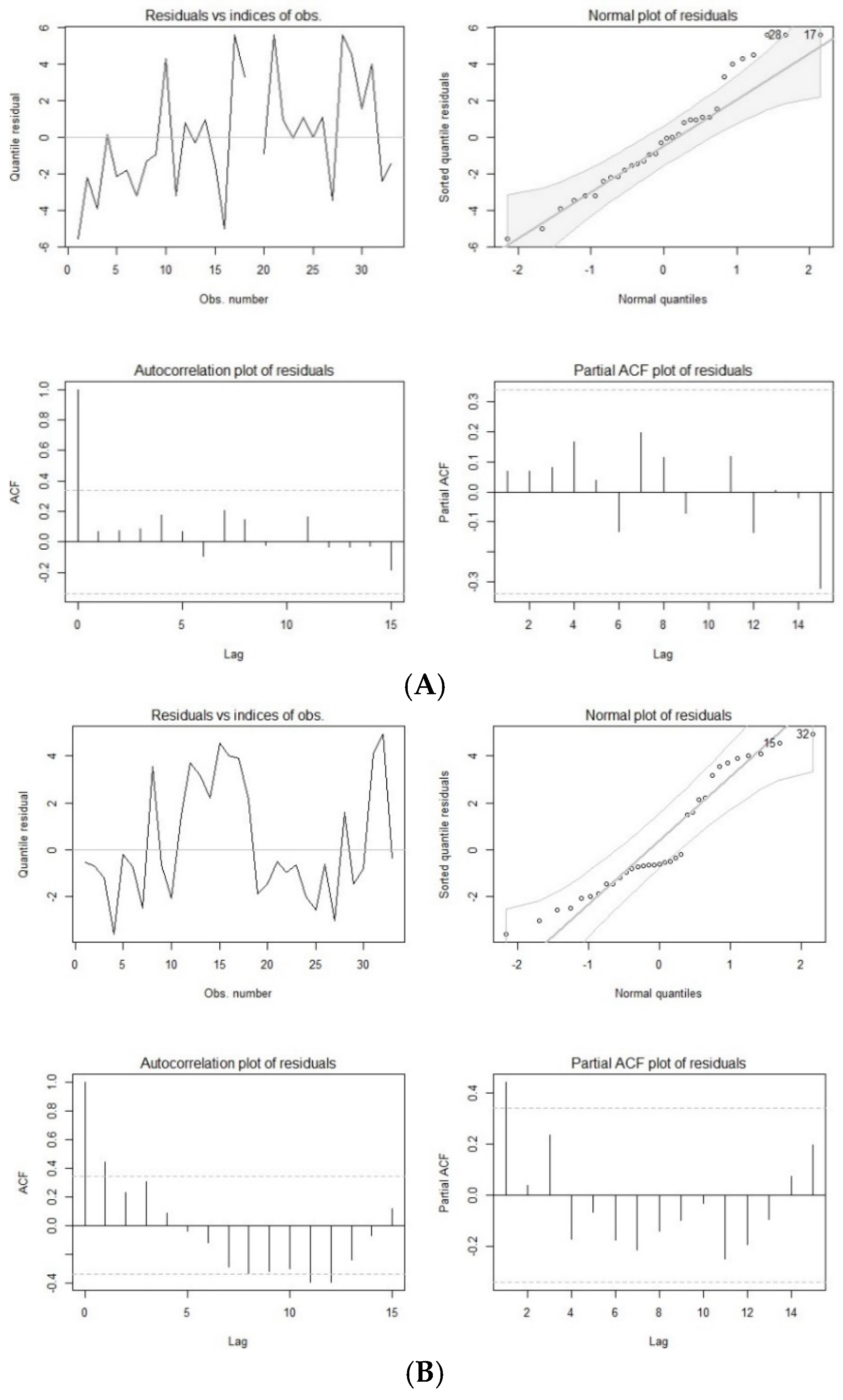
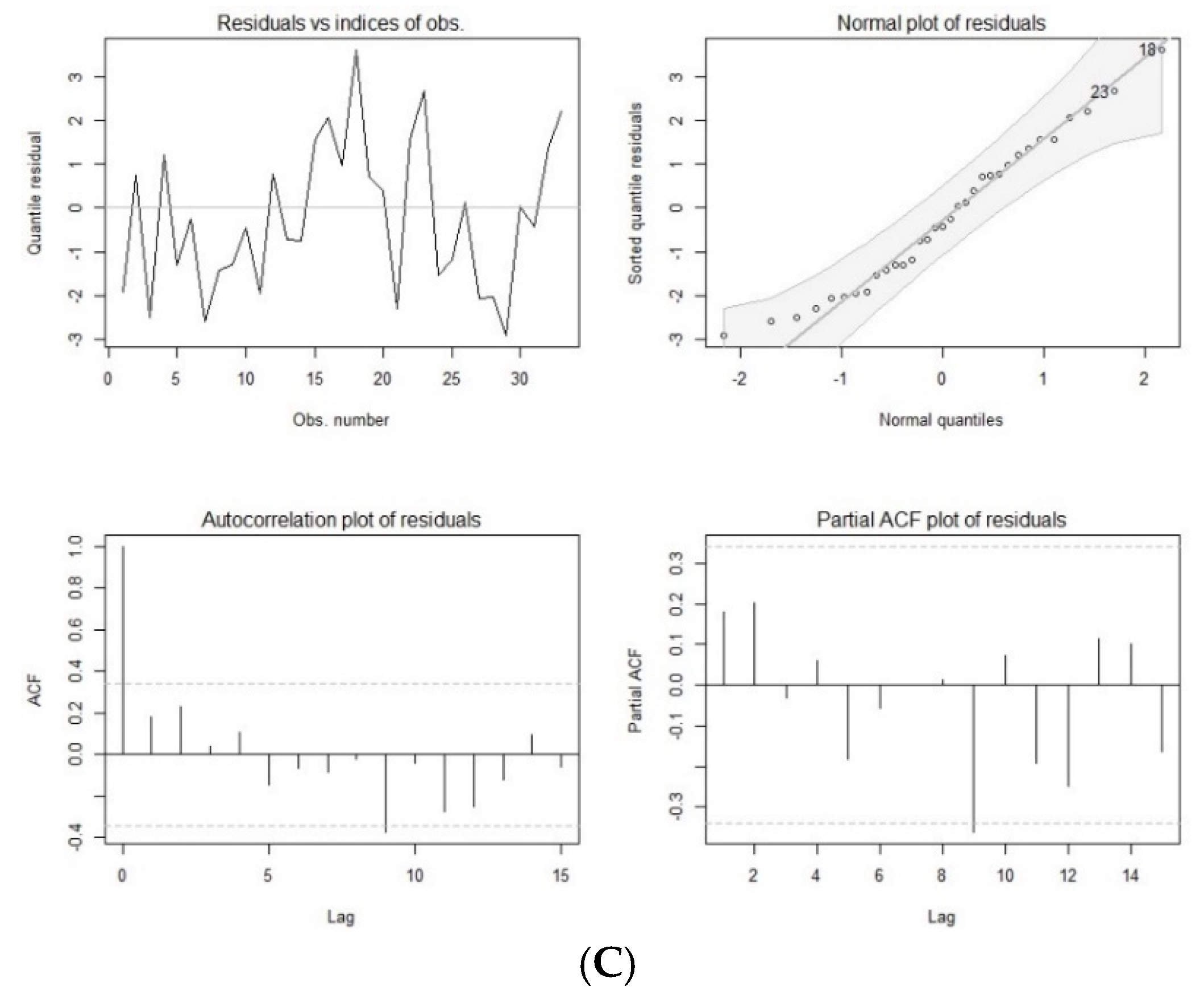
3.2. ARMA Time Series Analysis

The optimization analysis indicated that the combination of p = 1 and q = 1 was the optimal choice for the AR and MA parameters of the ARMA model, as determined by AIC values, dispersion parameters, and the coefficients of the AR and MA terms, respectively (Table 1). Using a Poisson distribution, the AIC values from the ARMA (1,1) model for COVID-19 cases, hospitalization cases, and death cases ranged from 165 to 356 with missing data, and from 188 to 595 with imputed data. Both the AR and MA parameters of the ARMA (1,1) model were statistically significant (p < 0.05) in the time series analyses for both missing and imputed data (Table 1). Using a negative binomial distribution, the AIC values from the ARMA (1,1) model for both missing and imputed data fell within a reasonable range, from 133 to 218. The dispersion parameters for COVID-19 cases, hospital admissions, and deaths were also significant for both missing and imputed data (Table 1).
This model was validated through multiple methods. First, the ACF plot suggested that the model was stationary, as the plot showed a relatively quick decay. Second, the PACF plot, used to assess the MA parameter, also indicated a quick decay after the cutoff point. Third, the qq-plots for the ARMA (1,1) model across all clinical case groups (with both missing and imputed data) exhibited 45-degree lines, and the residual plots for imputed data fell within a narrow interval (Figure 1). The qq-plots and residual plots confirmed that the ARMA (1,1) model was appropriate for predicting trends in the clinical cases (Figure 1). The optimization analysis and modeling validation supported that the ARMA (1,1) model was used and integrated in the CTS marginal regression model for forecasting the clinical cases.

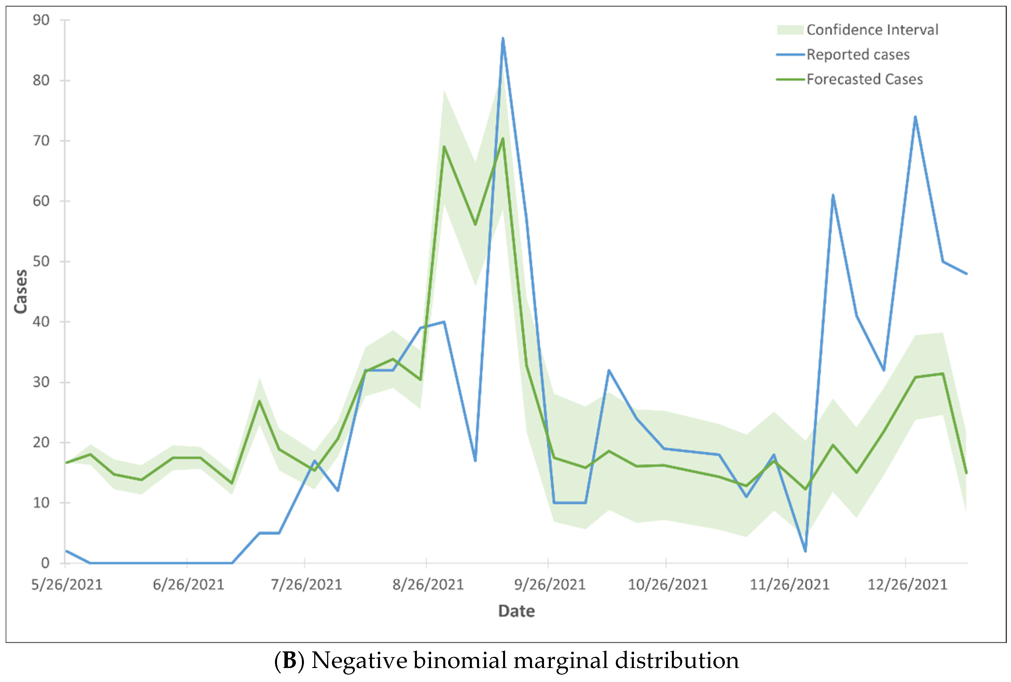
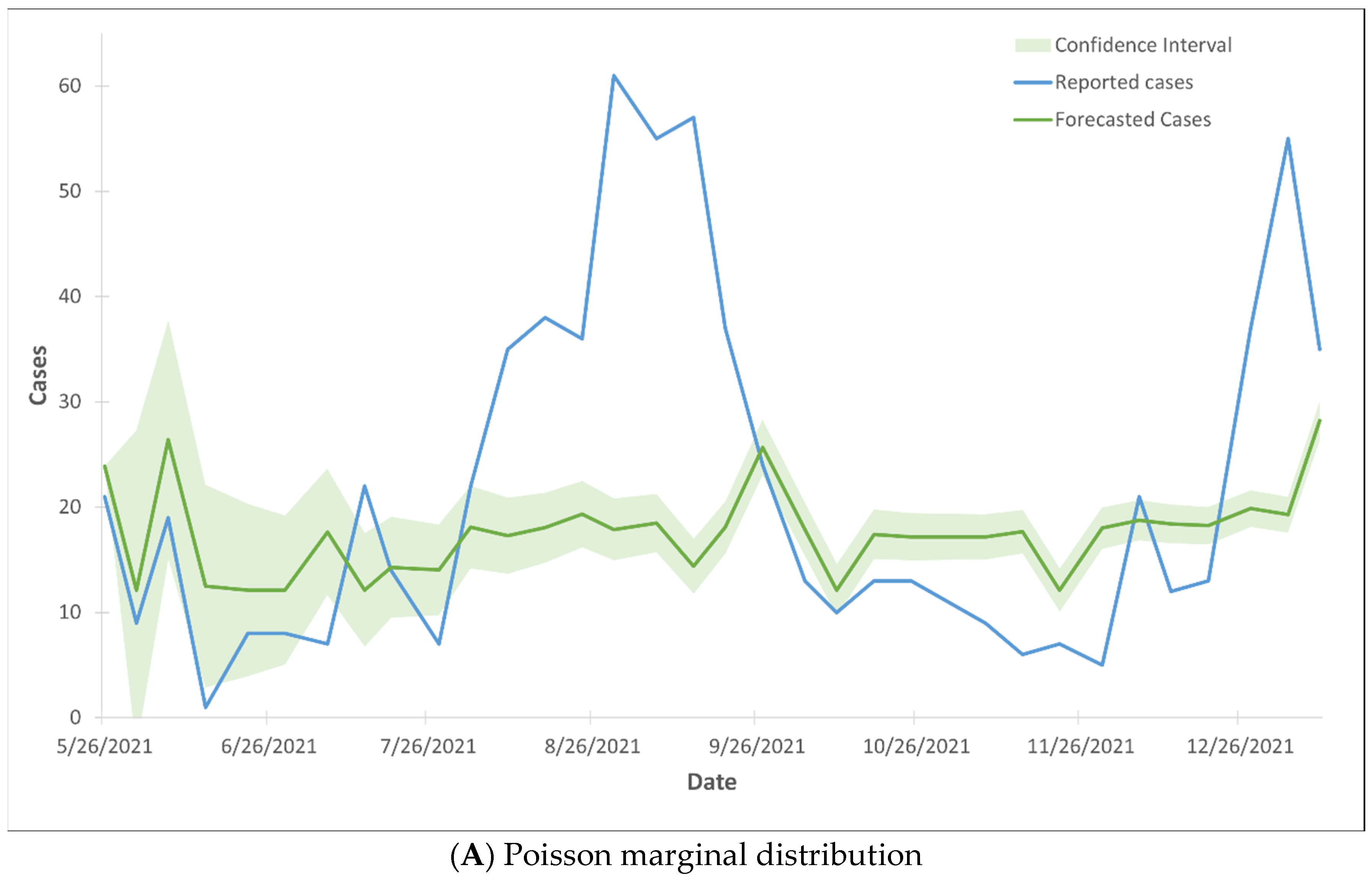
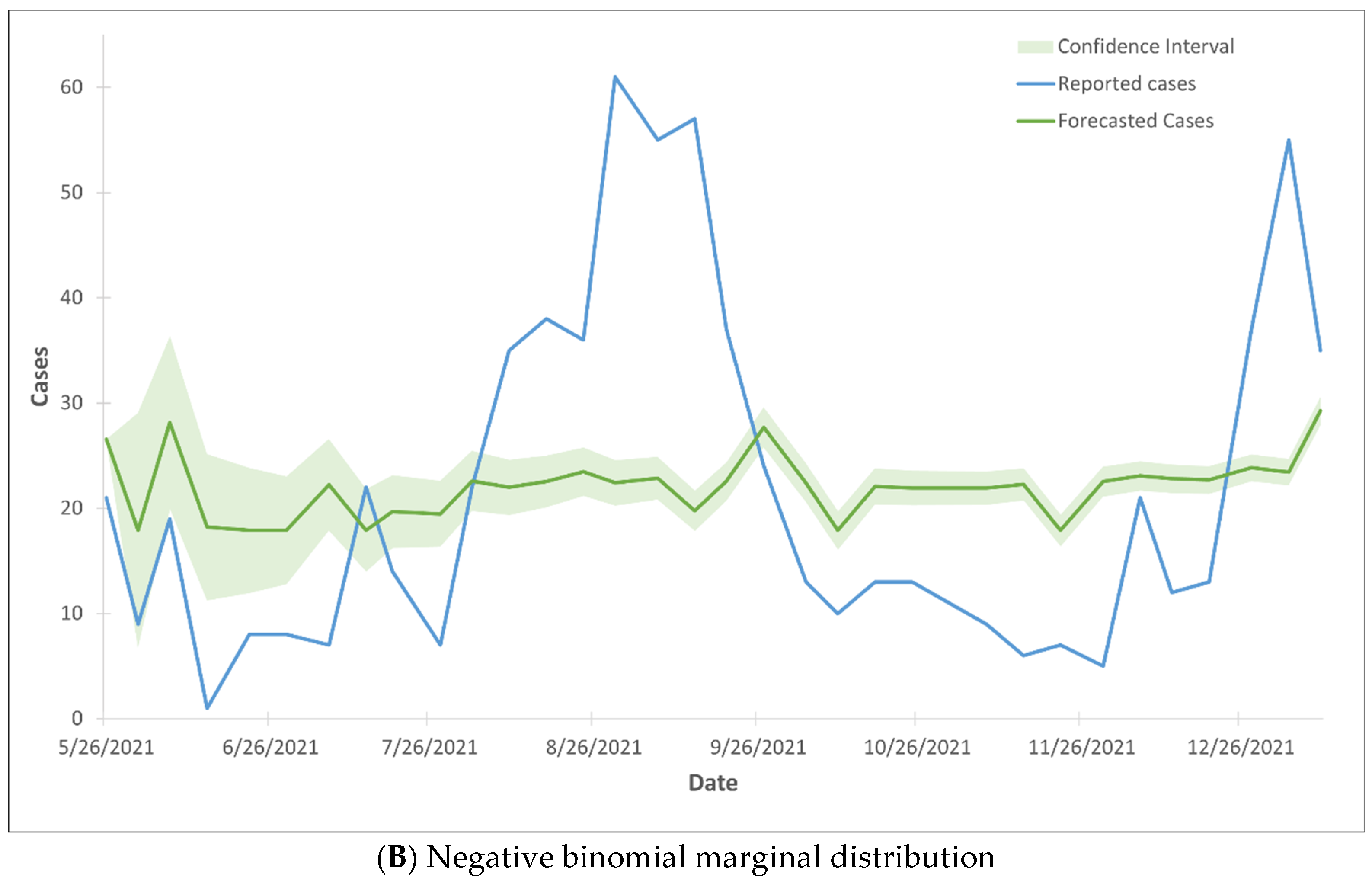
3.3. Modeling COVID-19 Cases

The forecasted COVID-19 cases, generated using the CTS marginal regression model, closely corresponded to the reported cases, as they fell within the 99% confidence interval (Figure 1). The observation held true for both Poisson marginal and negative binominal marginal distributions. Over 96% of the observations fall within the 99% confidence intervals, with the exception of the months of June and July. During these two months, only 27% of the observations fell within the 99% confidence interval (Figure 2).

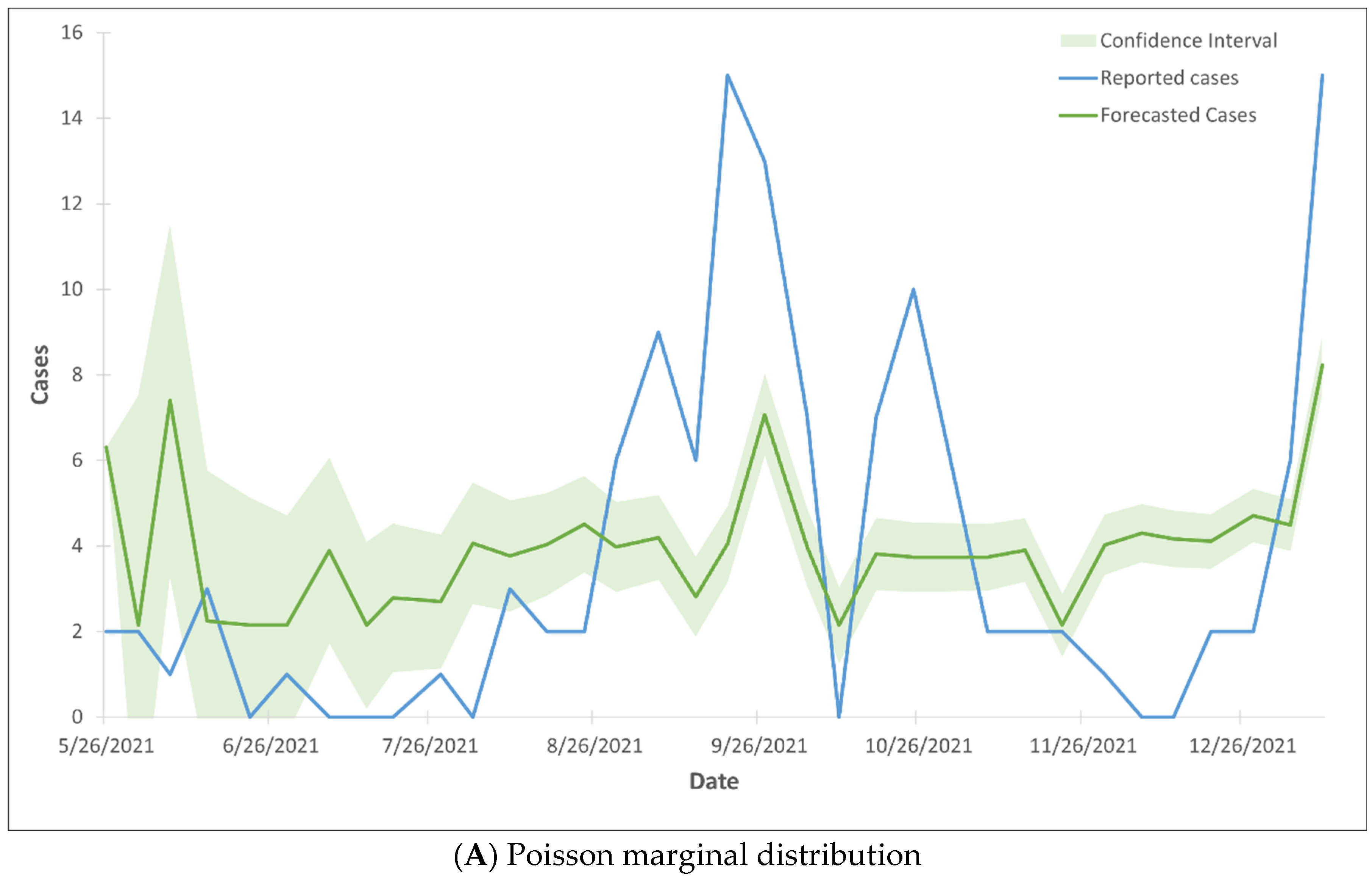
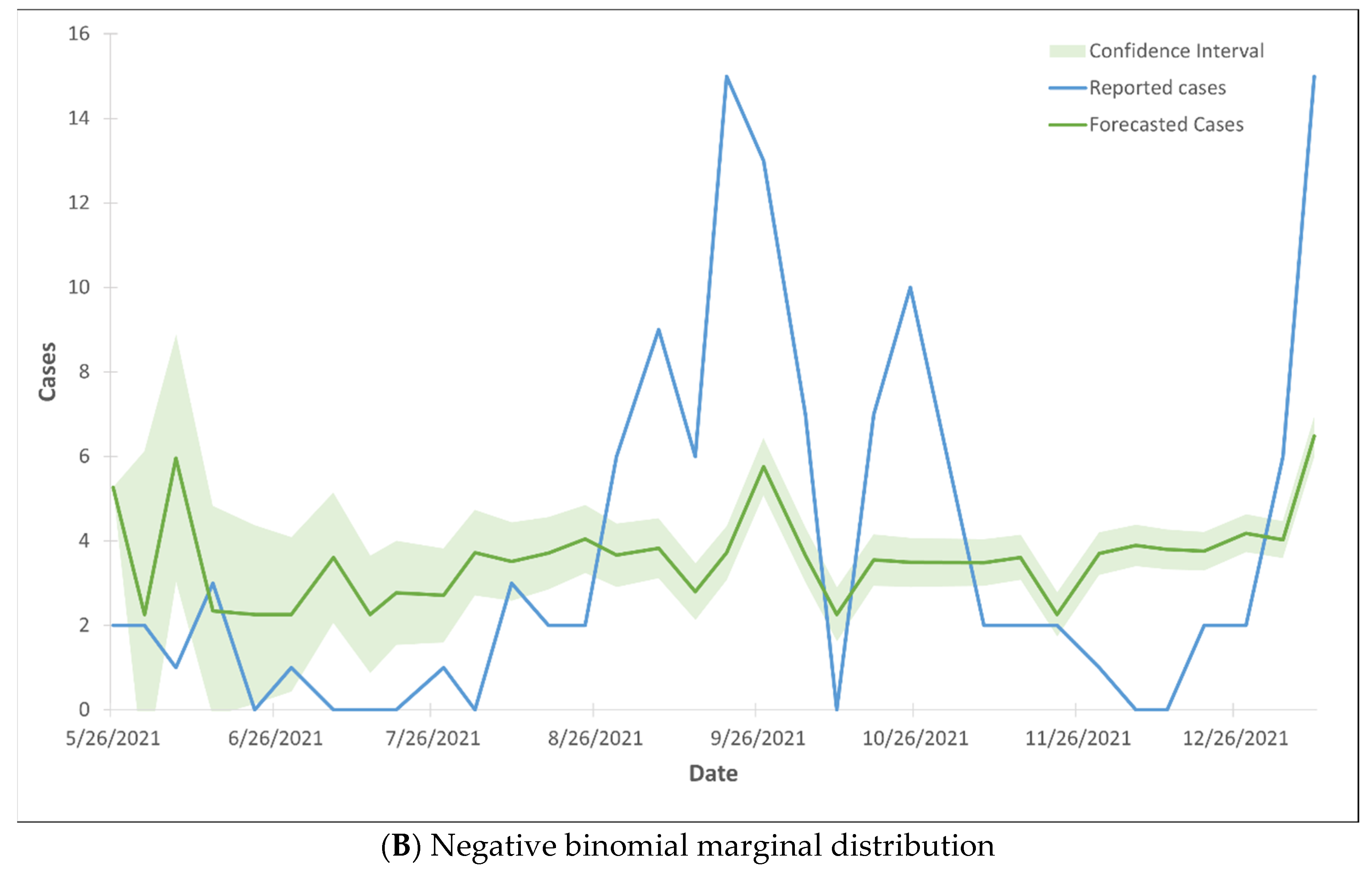
3.4. Modeling Hospital Admissions

The forecasted hospital admissions did not align with the reported cases, as the majority of the forecasted cases fell outside the 99% confidence interval range (Figure 3). The Gaussian CTS marginal regression models with both Poisson and negative binomial marginal distributions did not predict the rise in hospital admissions.

3.5. Modeling Death Cases

The forecasted death cases did not align with the reported cases, as the majority of the forecasted cases fell outside the 99% confidence interval range (Figure 4). The Gaussian CTS marginal regression models with both Poisson and negative binomial marginal distributions did not predict the rise in death cases.

4. Discussion

The Gaussian CTS marginal regression model was employed to address the non-normal distributions of wastewater SARS-CoV-2 viral load and clinical cases, as well as the time-dependent nature of discrete variables. An innovative aspect of this work is the inclusion of hospital admissions and deaths. Additionally, this model can capture the correlation between wastewater viral load and clinical cases. A strong correlation was observed between wastewater SARS-CoV-2 viral load and COVID-19 cases, consistent with findings reported in previous studies [7,9]. However, the correlations between wastewater viral load and hospital admissions or deaths were weak. This disparity may be attributed to the wide availability of vaccines. Additionally, a large number of zero cases, particularly for deaths, were recorded. Although the PMM imputation technique was applied to address the prevalence of zero cases, it could not fully overcome the limitations of the dataset.
The ARMA model played a crucial role in the Gaussian CST marginal regression model by examining the marginal distribution of each variable. Both Poisson and negative binomial distributions were evaluated to determine the most suitable condition for using an ARMA model to forecast clinical cases. The inclusion of the negative binomial distribution was particularly significant, as it contributes to the limited body of research currently available on forecasting clinical cases. Robust validation approaches, including Gaussian copula marginal regression (GCMR) residual analysis, QQ plots, and ACF/PACF plots, were employed to validate the ARMA model’s suitability for forecasting. To select the best-fit model, the combination p and q order was examined to identify the optimal values for forecasting. The ARMA (1,1) model emerged as the best fit, striking a balance between model accuracy and complexity. Residual plots in Figure 1 further justified the selected models for both reported and forecasted cases. These plots demonstrate that the sample autocorrelations for lags −10 to 5 do not exceed the significance bounds, supporting the validity of the chosen ARMA (1,1) model.
The integration of Poisson and negative binomial ARMA (1,1) models with the Gaussian copula demonstrated that the Gaussian CTS Marginal Regression model was capable of forecasting clinical cases, particularly COVID-19 cases, using wastewater SARS-CoV-2 viral load as a key predictor. Gaussian copula was chosen for its simplicity, though ongoing research continues to explore alternative copula models.
The marginal regression model could predict the trends of COVID-19 and rising numbers of cases. In predicting COVID-19 cases, the negative binomial outperformed Poisson in either missing or imputed data. However, the model with both Poisson and negative binomial marginal distributions occasionally overestimated or underestimated the reported cases. The discrepancy may be due to the time lag in reported cases or underreported cases, personal behaviors [24], vaccination [25], and herd immunity [26]. The forecasting model revealed that predicted COVID-19 cases were approximately 5 to 8 days earlier than clinical records. Several previous studies have observed similar results, indicating that an up-to-one-week-long lag period occurs between the increase in wastewater SARS-CoV-2 viral load and the subsequent rise in reported clinical PCR test cases [3,10,12,23,27].
Although the forecasting model was validated with low AIC values and normally distributed residual errors, the models in both Poisson and negative binomial did not effectively predict trends in hospital admissions and death cases. Specifically, the Poisson and negative binomial models failed to capture spikes in these outcomes, likely due to variations in lag times between RNA detection in wastewater and subsequent hospitalizations or deaths. After vaccines became widely available, hospital admissions and death cases declined significantly, leading to smaller sample sizes and an increased presence of zero cases. These data limitation reduced the accuracy of the forecasts, particularly for death case trends. While Gaussian copula helped manage extreme observations, biases may still be present in the forecasting outcomes.
Modeling COVID-19 cases and trends using wastewater viral load presents significant challenges due to the time-dependent nature of the data, the presence of missing and zero observations, and the complex dynamic of the pandemic. The new forecasting model introduced several strengths and innovations. While traditional time series models perform well with large datasets containing minimal missing data, copula-based approaches offer a more robust alternative for modeling clinical data related to the COVID-19 pandemic. Because clinical cases—including COVID-19 diagnoses, hospital admissions, and deaths—are temporally dependent, GCMR can effectively capture and incorporate these correlations under non-linear terms in the forecast modeling. The copula can combine the joint distributions of two variables, such as wastewater SARS-CoV-2 viral load and COVID-19 cases or hospital admissions, allowing for making inferences of predicted values of clinical cases.
Another key strength of this approach was its ability to handle sparse missing data more effectively. Our model demonstrated that accurate inference and prediction remain achievable even when assumptions of normality and data continuity are violated. Additionally, the Gaussian CTS marginal regression model offers the flexibility to extend from single-variable regression to multivariate analysis while preserving the ability to specify marginal distributions [28,29]. This adaptability is particularly useful for complex applications such as longitudinal data analysis, spatial statistics, and time series modeling [28,29,30].
The application of Gaussian copula has limitations, including (1) the lack of tail dependence, (2) the inability to handle asymmetric dependence, and (3) the difficulty in accurately capturing extreme numbers of rising cases [31]. However, these limitations did not significantly affect the forecasting capacity of the Gaussian CTS marginal regression model, as evidenced by COVID-19 cases forecasting (Figure 2). Specific limitations of the Gaussian CTS marginal regression model include (1) a limited amount of data at prediction times [32], (2) a lack of additional relevant variables related to clinical cases [27,33,34,35,36,37,38], (3) a high number of zero cases [39], (4) uncontrolled factors associated with the COVID-19 pandemic, and (5) the linear correlation between clinical cases and wastewater SARS-CoV-2 levels [40]. Ongoing research aims to address these limitations to enhance its forecasting power.
To improve the predictive powers of the Gaussian CTS marginal regression model, future studies can include additional relevant covariates that are associated with the COVID-19 distribution and infection, such as comorbidity [27], age [33,34], race [35,36,37], or socio-economic status [38]. These covariates should be incorporated into the development of modeling. Also, extending the length of the study period can increase the model’s predictive powers. The current study lasted for one year, during which both wastewater and clinical data were varying simultaneously. Larger data can enhance the prediction power of the models. By extending the study length in this the complex model, the autoregressive integrated moving average model can take seasonal effect into account. Finally, implementing a zero-inflation function in the model can help address the bias caused by a large number of zero cases observed in certain periods, particularly in hospital admissions and deaths after vaccination [39].
The transmission dynamics of SARS-CoV-2 and the COVID-19 pandemic are complex, leading to inherent limitations in modeling. One key limitation is the small number of clinical cases, which may impact the model’s predictive accuracy. A large number of zero cases in hospital admissions and deaths further reduces the model’s accuracy. Forecasting models generally require large datasets to enhance precision. However, despite this constraint, the use of copulas for time series has proven to be a valid approach for constructing forecasting models. These models may still possess sufficient power to predict cases and trends effectively. The second limitation concerns seasonal patterns. The autoregressive component of the ARMA model is most reliable when seasonal fluctuations influence the underlying factors of COVID-19 cases and trends. Ongoing research contributes to exploring seasonal pattern effects on the model performance. Third, local public health policies, such as lockdowns, re-opening of local activities, and traveler movement, may have introduced inconsistencies in the prediction outcomes. Fourth, variables related to personal behaviors were not included in the study, which could contribute to case spikes and affect the model parameters, particularly the variance of the error terms. Finally, changes in vaccination status during the study period may also have impacted the results.

5. Conclusions

SARS-CoV-2 viral loads in wastewater were found to correlate with reported COVID-19 cases, consistent with previous studies [6,7,8,9]. Also, the study introduced a new finding: a correlation between SARS-CoV-2 viral loads in wastewater and hospital admissions. The CTS marginal regression model, which combines the ARMA model and the copula function, was successfully developed and validated for time series forecasting. Notably, this model demonstrated the ability to forecast COVID-19 cases and trends using only SARS-CoV-2 viral load in wastewater. The model using wastewater data only has significant predictive power and accuracy for clinical data forecasting, offering valuable potential for COVID-19 control and broader public health applications. Wastewater surveillance has been recommended as an effective monitoring tool for detecting the presence of COVID-19 and informing public health responses. The CTS marginal regression model could enhance the efficiency and accuracy of wastewater surveillance by forecasting COVID-19 trends across specific and large geographic areas, providing lead time prior to hospital admissions.

Author Contributions

Conceptualization, H.A.J. and N.D.; methodology: H.A.J., N.D., K.C. and R.G.; software, N.D. and S.A.; validation, N.W., C.J. and R.S.; resources, D.J. and R.S.; writing, H.A.J. and N.D.; project administration, H.A.J.; funding acquisition, R.S. All authors have read and agreed to the published version of the manuscript.

Funding

The project was supported by the Data Science Seed Funding and the School of Public Health Initiative Grant from Old Dominion University.

International Review Board Statement

Not applicable.

Informed Consent Statement

Not applicable.

Data Availability Statement

All data generated and analyzed during this study are included in this article. The authors do not have permission to share raw data.

Acknowledgments

We acknowledge the staff and laboratory technicians from the Hampton Roads Sanitation District for wastewater sampling and SARS-CoV-2 analysis. Also, we thank the staff from the Chesapeake Health Department for participating in data interpretation.

Conflicts of Interest

The authors declare that they have no known competing financial interests that could have appeared to influence the work reported in this paper.

References

  1. Agrawal, S.; Orschler, L.; Lackner, S. Long-term monitoring of SARS-CoV-2 RNA in wastewater of the Frankfurt Metropolitan A in southern Germany. Sci. Rep. 2021, 11, 5372. [Google Scholar] [CrossRef] [PubMed]
  2. Gonzalez, R.; Curtis, K.; Bivins, A.; Bibby, K.; Weir, M.H.; Yetka, K. COVID-19 surveillance in southeastern Virginia using wastewater-based epidemiology. Water Res. 2020, 186, 116296. [Google Scholar] [CrossRef] [PubMed]
  3. Parasa, S.; Desai, M.; Thoguluva Chandrasekar, V.; Patel, H.K.; Kennedy, K.F.; Roesch, T.; Spadaccini, M.; Colombo, M.; Gabbiadini, R.; Artifon, E.L.A.; et al. Prevalence of gastrointestinal symptoms and fecal viral shedding in patients with coronavirus disease 2019: A systematic review and meta-analysis. JAMA Netw. Open 2020, 3, e2011335. [Google Scholar] [CrossRef]
  4. Peccia, J.; Zulli, A.; Brackney, D.E.; Grubaugh, N.D.; Kaplan, E.H.; Casanovas-Massana, A.I.; Ko, A.A.; Malik, D.; Wang, M.; Warren, J.L. Measurement of SARS-CoV-2 RNA in wastewater tracks community infection dynamics. Nat. Biotechnol. 2020, 38, 1164–1167. [Google Scholar] [CrossRef] [PubMed]
  5. Tang, A.; Tong, D.; Wang, H.L.; Dai, Y.X.; Li, K.F.; Liu, J.N.; Wu, W.J.; Yuan, C.Y.; Yu, M.L.; Li, P.; et al. Detection of novel coronavirus by RT-PCR in stool specimen from asymptomatic child, China. Emerg. Infect. Dis. 2020, 26, 1337–1339. [Google Scholar] [CrossRef] [PubMed]
  6. Wu, F.; Zhang, J.; Xiao, A.; Gu, X.; Lee, W.L.; Armas, F.; Kauffman, K.; Hanage, W.; Matus, M.; Ghaeli, N.; et al. SARS-CoV-2 titers in wastewater are higher than expected from clinically confirmed cases. mSystems 2020, 5, e00614. [Google Scholar] [CrossRef]
  7. Markt, R.; Endler, L.; Amman, F.; Schedl, A.; Penz, T.; Büchel-Marxer, M.; Grünbacher, D.; Mayr, M.; Peer, E.; Pedrazzini, M.; et al. Detection and abundance of SARS-CoV-2 in wastewater in Liechtenstein, and the estimation of prevalence and impact of the B. 1.1.7 variant. J. Water Health 2022, 1, 114–125. [Google Scholar] [CrossRef]
  8. Trottier, J.; Darques, R.; Ait Mouheb, N.; Partiot, E.; Bakhache, W.; Deffieu, M.S.; Gaudin, R. Post-lockdown detection of SARS-CoV-2 RNA in the wastewater of Montpellier, France. One Health 2020, 10, 100157. [Google Scholar] [CrossRef] [PubMed]
  9. Jeng, H.A.; Singh, R.; Diawara, N.; Curtis, K.; Gonzalez, R.; Welch, N.; Jackson, C.; Jurgens, D.; Adikari, S. Application of wastewater-based surveillance and copula time-series model for COVID-19 forecasts. Sci. Total Environ. 2023, 885, 163655. [Google Scholar] [CrossRef]
  10. D’Aoust, P.M.; Mercier, E.; Montpetit, D.; Jia, J.J.; Alexandrov, I.; Neault, N.; Baig, A.T.; Mayne, J.; Zhang, X.; Alain, T.; et al. Quantitative analysis of SARS-CoV-2 RNA from wastewater solids in communities with low COVID-19 incidence and prevalence. Water Res. 2021, 188, 116560. [Google Scholar] [CrossRef]
  11. Róka, E.; Khayer, B.; Kis, Z.; Kovács, L.B.; Schuler, E.; Magyar, N.; Málnási, T.; Oravecz, O.; Pályi, B.; Pándics, T.; et al. Ahead of the second wave: Early warning for COVID-19 by wastewater surveillance in Hungary. Sci. Total Environ. 2021, 786, 147398. [Google Scholar] [CrossRef] [PubMed]
  12. Kisand, V.; Laas, P.; Palmik-Das, K.; Panksep, K.; Tammert, H.; Albreht, L.; Allemann, H.; Liepkalns, L.; Vooro, K.; Ritz, C.; et al. Prediction of COVID-19 positive cases, a nation-wide SARS-CoV-2 wastewater-based epidemiology study. Water Res. 2023, 231, 119617. [Google Scholar] [CrossRef] [PubMed]
  13. Wurtz, N.; Lacoste, A.; Jardot, P.; Delache, A.; Fontaine, X.; Verlande, M.; Annessi, A.; Giraud-Gatineau, A.; Chaudet, H.; Fournier, P.E.; et al. Viral RNA in city wastewater as a key indicator of COVID-19 recrudescence and containment measures effectiveness. Front. Microbiol. 2021, 12, 664477. [Google Scholar] [CrossRef]
  14. Daza-Torres, M.L.; Montesinos-López, J.C.; Kim, M.; Olson, R.; Bess, C.W.; Rueda, L.; Susa, M.; Tucker, L.; García, Y.E.; Schmidt, A.J.; et al. Model training periods impact estimation of COVID-19 incidence from wastewater viral loads. Sci. Total Environ. 2023, 858, 159680. [Google Scholar] [CrossRef]
  15. Taghia, J.; Kulyk, V.; Ickin, S.; Folkesson, M.; Nyström, C.; Ȧgren, K.; Brezicka, T.; Vingasre, T.; Karlsson, J.; Fritzell, I.; et al. Development of forecast models for COVID-19 hospital admissions using anonymized and aggregated mobile network data. Sci. Rep. 2022, 12, 17726. [Google Scholar] [CrossRef] [PubMed]
  16. Galani, A.; Aalizadeh, R.; Kostakis, M.; Markou, A.; Alygizakis, N.; Lytras, T.; Adamopoulos, P.G.; Peccia, J.; Thompson, D.C.; Kontou, A.; et al. SARS-CoV-2 wastewater surveillance data can predict hospitalizations and ICU admissions. Sci. Total Environ. 2022, 804, 150151. [Google Scholar] [CrossRef]
  17. Nelsen, R.B. An Introduction to Copulas; Springer Science & Business Media: Berlin/Heidelberg, Germany, 2007. [Google Scholar]
  18. Sen, S.; Diawara, N. Supervised Classification Using Finite Mixture Copula. J. Probab. Stat. Sci. 2017, 15, 189–201. [Google Scholar]
  19. Shahriari, S.; Sisson, S.A.; Rashidi, T. Copula ARMA-GARCH modeling of spatially and temporally correlated time series data for transportation planning use. Transp. Res. Part C Emerg. Technol. 2023, 146, 103969. [Google Scholar] [CrossRef]
  20. Ekinci, A. Modelling and forecasting of growth rate of new COVID-19 cases in top nine affected countries: Considering conditional variance and asymmetric effect. Chaos Solitons Fractals 2021, 151, 111227. [Google Scholar] [CrossRef] [PubMed]
  21. Wulff, J.N.; Jeppesen, L.E. Multiple imputation by chained equations in praxis: Guidelines and review. Electron. J. Bus. Res. Methods 2017, 15, 41–56. [Google Scholar]
  22. Alzahrani, S.I.; Aljamaan, I.A.; Al-Fakih, E.A. Forecasting the spread of the COVID-19 pandemic in Saudi Arabia using ARIMA prediction model under current public health interventions. J. Infect. Public Health 2020, 13, 914–919. [Google Scholar] [CrossRef] [PubMed]
  23. Tounkara, F.; Lefebvre, G.; Greenwood, C.; Oualkacha, K. A flexible copula-based approach for the analysis of secondary phenotypes in ascertained samples. Stat. Med. 2020, 39, 517–543. [Google Scholar] [CrossRef] [PubMed]
  24. Aouissi, H.A.; Kechebar, M.S.A.; Ababsa, M.; Roufayel, R.; Neji, B.; Petrisor, A.I.; Hamimes, A.; Epelboin, L.; Ohmagari, N. The Importance of behavioral and native factors on COVID-19 infection and severity: Insights from a preliminary cross-sectional study. Healthcare 2022, 10, 1341. [Google Scholar] [CrossRef]
  25. Plescia, M.; Hannan, C.; Baggett, J. A pandemic success story: Distribution and administration of COVID-19 vaccines. J. Public Health Manag. Pract. 2022, 28, 749–750. [Google Scholar] [CrossRef]
  26. Suryawanshi, Y.; Biswas, D.A. Herd immunity to fight against COVID-19: A narrative review. Cureus 2023, 15, e33575. [Google Scholar] [CrossRef]
  27. Gasmi, A.; Peana, M.; Pivina, L.; Srinath, S.; Benahmed, G.A.; Semenova, Y.; Menzel, A.; Dadar, M.; Bjørklund, G. Interrelations between COVID-19 and other disorders. Clin. Immunol. 2021, 224, 108651. [Google Scholar] [CrossRef] [PubMed]
  28. Masarotto, G.; Varin, C. Gaussian copula regression in R. J. Stat. Softw. 2017, 77, 1–26. [Google Scholar] [CrossRef]
  29. Song, P.X.-K. Multivariate dispersion models generated from Gaussian copula. Scand. J. Stat. 2020, 27, 305–320. [Google Scholar] [CrossRef]
  30. Guolo, A.; Varin, C. Beta regression for time series analysis of bounded data, with application to Canada Google Flu Trends. Ann. Appl. Stat. 2014, 8, 74–88. [Google Scholar] [CrossRef]
  31. Henn, L.L. Limitations and performance of three approaches to Bayesian inference for Gaussian copula regression models of discrete data. Comput. Stat. 2022, 37, 909–946. [Google Scholar] [CrossRef]
  32. Suresh, K.; Taylor, J.M.G.; Tsodikov, A. A Gaussian copula approach for dynamic prediction of survival with a longitudinal biomarker. Biostatistics 2019, 22, 504–521. [Google Scholar] [CrossRef]
  33. Smith, M.; Abdesselem, H.B.; Mullins, M.; Tan, T.M.; Nel, A.J.M.; Al-Nesf, M.A.Y.; Bensmail, I.; Majbour, N.K.; Vaikath, N.N.; Naik, A.; et al. Age, disease severity and ethnicity influence humoral responses in a multi-ethnic COVID-19 cohort. Viruses 2021, 13, 786. [Google Scholar] [CrossRef] [PubMed]
  34. Akpinar, G.; Demir, M.C.; Sultanoglu, H.; Sonmez, F.T.; Karaman, K.; Keskin, B.H.; Ince, N.; Guclu, D. The demographic analysis of the probable COVID-19 cases in terms of RT-PCR results and age. Clin. Lab. 2021, 67, 1058. [Google Scholar] [CrossRef] [PubMed]
  35. Raine, S.; Liu, A.; Mintz, J.; Wahood, W.; Huntley, K.; Haffizulla, F. Racial and ethnic disparities in COVID-19 Outcomes: Social Determination of Health. Int. J. Environ. Res. Public Health 2020, 17, 8115. [Google Scholar] [CrossRef] [PubMed]
  36. Mahajan, U.V.; Larkins-Pettigrew, M. Racial demographics and COVID-19 confirmed cases and deaths: A correlational analysis of 2886 US counties. J. Public Health 2020, 42, 445–447. [Google Scholar] [CrossRef]
  37. Xu, A.; Loch-Temzelides, T.; Adiole, C.; Botton, N.; Dee, S.G.; Masiello, C.A.; Osborn, M.; Torres, M.A.; Cohan, D.S. Race and ethnic minority, local pollution, and COVID-19 deaths in Texas. Sci. Rep. 2022, 12, 1002. [Google Scholar] [CrossRef] [PubMed]
  38. Hawkins, R.B.; Charles, E.J.; Mehaffey, J.H. Socio-economic Status and COVID-19-Related Cases and Fatalities. Public Health 2020, 189, 129–134. [Google Scholar] [CrossRef] [PubMed]
  39. Alqawba, M.; Diawara, N. Copula-based Markov zero-inflated count time series models with application. J. Appl. Stat. 2021, 48, 786–803. [Google Scholar] [CrossRef]
  40. Ashrafi, M.; Soltanian-Zadeh, H. Multivariate Gaussian copula mutual information to estimate functional connectivity with less random architecture. Entropy 2022, 24, 631. [Google Scholar] [CrossRef]
Figure 1. Residual plots of autoregressive moving average model with Poisson distribution of COVID-19 cases (A), hospital admissions (B), and deaths (C) with imputed data.
Covid 05 00025 g001aCovid 05 00025 g001b
Figure 2. 99% confidence interval of the trend lines of forecasted COVID-19 cases using Gaussian CTS marginal regression model with imputed cases and by Poisson marginal distribution (A) and negative binominal marginal distribution (B).
Covid 05 00025 g002aCovid 05 00025 g002b
Figure 3. 99% confidence interval of the trend lines of hospital admission cases using Gaussian CTS marginal regression model with imputed cases and by Poisson marginal distribution (A) and negative binominal marginal distribution (B).
Covid 05 00025 g003aCovid 05 00025 g003b
Figure 4. 99% confidence interval of the trend lines of death cases using Gaussian CTS marginal regression model with imputed cases and by Poisson marginal distribution (A) and negative binominal marginal distribution (B).
Covid 05 00025 g004aCovid 05 00025 g004b
Table 1. Parameters estimations from Poisson ARMA (1,1) and Negative Binomial ARMA (1,1) for clinical cases.
COVID-19 CasesHospital AdmissionsDeaths
AICDispersion ParametersGaussian Copula Coefficients (AR, MA) with SignificanceAICDispersion ParametersGaussian Copula Coefficients (AR, MA) with SignificanceAICDispersion ParametersGaussian Copula Coefficients (AR, MA) with Significance
Poisson ARMA (1,1)
with missing data
356.04 0.71   * , 0.26   * 340.43 (0.51 *, −0.21)165.11 (0.67 *, −0.38 *)
Negative Binomial ARMA (1,1)
with missing data
195.11 1.48 ( 0.78   * , 0.04 ) 218.960.42 *(0.76 *, −0.21)133.221.17(0.77 *, −0.33)
Poisson ARMA (1,1)
with imputed data
596.15 ( 0.81   * , 0.55   * ) 409.46 (0.49 *, −0.23)188.75 (0.64 *, −0.37 *)
Negative Binomial ARMA (1,1)
with imputed data
255.93 1.87 ( 0.90   * , 0.42   * ) 253.990.42 *(0.71 *, −0.14)155.800.85 *(0.71 *, −0.29)
* Significance p < 0.05 .
Disclaimer/Publisher’s Note: The statements, opinions and data contained in all publications are solely those of the individual author(s) and contributor(s) and not of MDPI and/or the editor(s). MDPI and/or the editor(s) disclaim responsibility for any injury to people or property resulting from any ideas, methods, instructions or products referred to in the content.

