Abstract
Eddy covariance measurements are increasingly utilized for assessing the exchange of matter and energy between ecosystems and the atmosphere across various time scales, ranging from hours to years. The flux footprint represents the area observable by flux tower sensors and illustrates how the surface influences the measured flux. Flux footprint models describe both the spatial extent and the specific location of the surface area contributing to the observed turbulent fluxes. In this study, we applied a simple two-dimensional parameterization for flux footprint prediction (FFP), developed by Kljun et al. to identify the location of peak footprint contribution every half hour over a six-year period. Monthly cluster analysis was performed on these data. Using an open-source geographic information system (GIS) software, the resulting clusters were overlaid on a base map of the site obtained from the Estonian Land Board, where different compartments have varying growth stages and species compositions. Our main objective was to integrate forest inventory data with ecosystem exchange and productivity data continuously recorded by the eddy covariance measurement tower at Järvselja, Estonia. This integration enabled spatially explicit visualization of half-hourly flux contributions using geographic information system software.
1. Introduction
Forest ecosystems are crucial in shaping both local and global climates by managing the exchange of energy and matter between the atmosphere, vegetation and soil [1]. However, the role of forests as global carbon sink and in the regulation of natural aerosol load, cloud formation processes, energy and matter exchange, water cycle, air quality and climate mitigation are complex and yet not fully understood.
In recent years, eddy covariance (EC) measurements have become a preferred method for evaluating the exchange of matter and energy between ecosystems and the atmosphere over various time scales, from hours to years [2,3]. These flux measurements, conducted over different ecosystem time frames and spatial areas, help us understand ecosystem processes and their responses to changing biophysical conditions such as light, temperature, precipitation, soil moisture, CO2 levels, phenology and plant functional traits [3]. Long-term environmental measurements from SMEAR (Station for Measuring Ecosystem–Atmosphere Relations) stations in Estonia and Finland [4,5] provide valuable insights into these processes and allow us to quantify the interactions between forest ecosystems and their environment. The ability to integrate fluxes over time and space, combined with machine learning techniques, high-resolution satellite data, images and spatial and temporal meteorological data, now allows us to study ecosystems from specific moments to extended periods [6,7,8]. Understanding the spatial distribution of atmospheric matter and quantifying it within ecosystems necessitates detailed ground-based and satellite observations enhanced by mathematical modeling [1].
The flux footprint outlines the area visible to flux tower sensors and indicates how the surface affects the measured flux. The flux footprint is influenced by measurement height, surface roughness, wind speed and direction and thermal stability [9,10]. Flux footprint models have been developed since the 1970s [11] and describe both the spatial extent and the location of the surface areas contributing to the measured turbulent flux at any given moment [7,12]. This study applies the two-dimensional flux footprint parameterization by Kljun et al. [7], which is based on Lagrangian stochastic modeling and captures both along-wind and crosswind dispersion. Kljun’s two-dimensional parameterization incorporates both measurement height and surface roughness into the FFP model [7]. Compared to the analytical model by Kormann & Meixner [13], it offers a broader applicability across atmospheric stability conditions and over heterogeneous terrain. Its simplified empirical formulation ensures realistic footprint estimates while maintaining computational efficiency, making it well-suited for long-term flux tower studies and automatized processing of large datasets.
The fluxes measured at the eddy covariance station are also affected by the spatial distribution and structure of forest elements, such as tree species composition and their developmental stages. Recent research on the footprint climatology’s variability in terms of spatial extent and time [14] has revealed that forest stand elements, such as clear-cut areas or stand thinning, change the structure within the footprint area by natural and man-made means on a small scale. This is especially true for forests that contain a high degree of natural elements, such as the Järvselja old-growth forest [15], which is part of the SMEAR Estonia’s flux tower footprint and exhibits a very fine-grained spatial variability of the forest elements that determine the area’s overall flux signature. Because the wind direction and speed are the major factors that determine where the maximal flux signal is located within the footprint area, meteorological large-scale events like prevailing wind directions that are linked to the global atmospheric transport or local scale storms lead to different spatial distributions of the measured flux.
To properly assess such spatially dynamic events, we also need to include information about the forest elements, including standing stock, species distribution and the age of the forest stands. Since 1999, the National Forest Inventory (NFI) has been carried out in Estonia to provide a comprehensive overview of the country’s forest resources [16,17]. The NFI offers detailed data on land distribution by land-use categories, afforestation trends and the growing stock of non-forest areas [18]. It also includes key stand structural attributes such as species composition, tree diameter, height, annual growth increment and stand volume, which are essential for characterizing forest structure and development across compartments. So far, integration of flux and biometrical data has been achieved by combining forest inventory measurements at the plot scale, such as aboveground biomass increment, tree-ring width, or wood density measurements [19,20]. However, the usual heterogeneity in most measurement sites is due to changing wind patterns, surface characteristics and differing species distributions [21,22], and it cannot be avoided. Estimating the location of the origin of most of the half-hourly flux data and the potential flux hotspots within the footprint therefore offers valuable information for carbon budgets.
We aim to develop a novel approach that utilizes the location of maximum footprint contribution in combination with unsupervised clustering algorithms to spatially link flux data with specific forest ecosystem features at the stand level. By integrating spatiotemporal datasets, this method will enable a finer scale understanding of forest processes and their spatial variability.
The footprint spatial representativeness is relevant in terms of upscaling, for example, when integrating in situ measurements with remote sensing [23] or when the footprint may contain point sources of GHG emissions [24]. Typical challenges are the possible heterogeneity within the footprint area and the changing source areas over time intervals.
2. Materials and Methods
2.1. Study Area
The SMEAR Estonia [4,5], located at 58.2714° N, 27.2703° E at 36 m a.s.l., is situated at the Järvselja Experimental Forestry Centre, which is the southernmost SMEAR station in the European SMEAR network (Figure 1). The forest around SMEAR Estonia can be classified as hemiboreal [5,25]. The experimental forest covers 10,408 hectares, of which 62.75% is forest. The forest has a mix of broad leaf and coniferous species such as birch species (Betula pendula and B. pubescens), Scots pine (Pinus sylvestris), Norway spruce (Picea abies), Aspen (Populus tremula) gray alder (Alnus incana) and black alder (A. glutinosa).
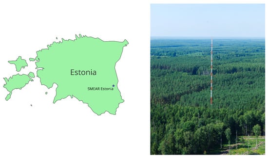
Figure 1.
Location of SMEAR Estonia and photo of the measurement tower.
The mean annual temperature is 4–6 °C, and mean annual precipitation is 500–750 mm, of which 40–80 mm is received as snow. The station has a 130 m high atmospheric measurement tower and a main cottage, which hosts the main power supply and power backup, provides internet access, a storage server for online data, controls for information technology solutions and the pumping facilities and gas analyzers for the large atmospheric mast [5].
2.2. Workflow Diagram
Figure 2 presents a schematic overview of data acquisition, integration processes and final outputs. Eddy covariance data were pre-processed using the REddyProc online tool [26], while forest inventory data, base maps and satellite imagery were obtained from the National Forest Register of Estonia (accessed on 28 February 2024). The green boxes highlight the specific steps undertaken in this study.
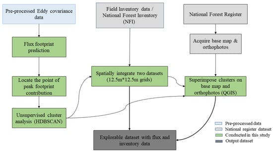
Figure 2.
The complete toolchain for the data integration and visualization is shown schematically.
2.3. Flux Measurement and Calculation
Since April 2014, the eddy covariance technique has been used to continuously measure CO2 and H2O fluxes at heights of 30 m and 70 m using METEK uSonic-3 Class A sonic anemometers (Elmshorn, Germany) and LI-COR LI-7200 gas analyzers (Lincoln, NE, USA). Additionally, greenhouse gas concentrations (CO2, H2O and CH4) have been monitored at five heights (30 m, 50 m, 70 m, 90 m and 110 m) since November 2015 with an LGR GGA analyzer (ABB, Zurich, Switzerland). All measurements were sampled at 10 Hz [5]. For this study, we used data from the 70 m level.
CO2 fluxes were calculated with EddyPro software (version 6.2.0, LI-COR, Lincoln, NE, USA) using the eddy covariance method [6,27,28], defined as the covariance between vertical wind velocity and CO2 concentration. The fluxes were averaged over 30 min intervals, and subsequent data processing was performed in MATLAB (Release R2013a & R2013b, The Mathworks, Inc., Natick, MA, USA) [29]. Net Ecosystem Exchange (NEE) was estimated as the sum of CO2 flux and storage, where storage was estimated as the average change in CO2 concentration within the air column below the measurement height over the corresponding time interval [29] and gap-filled using marginal distribution sampling [26,30] with the REddyProcWeb online tool [26,29]. Further details on instrumentation, data processing and gap-filling procedures are available in [5,29].
2.4. Footprint Calculation
Our flux footprint calculation was based on the two-dimensional parameterization for flux footprint prediction [7], and we employed the Python version 3.11.6 so we could automate the calculation for a large number of monthly datasets. Kljun’s FFP model enabled us to calculate a single footprint for every half hour, and a footprint climatology was calculated over longer time intervals (e.g., monthly or yearly) (Figure 3). The Kljun et al. [7] parameterization (FFP) is an empirical scaling model derived from a large ensemble of simulations using the Lagrangian stochastic particle dispersion model LPDM-B. It retains the physical realism of a Lagrangian framework while providing a computationally efficient, two-dimensional approximation that captures both the along-wind and crosswind structures of the footprint. FFP is explicitly validated for a wide range of boundary-layer conditions (convective, neutral and stable), receptor heights up to the full planetary boundary layer and surface roughness lengths from smooth to forested surfaces. Importantly, the model explicitly includes the effects of surface roughness length (z0) and Obukhov length (ol) through dimensionless scaling parameters, ensuring realistic footprint behavior across varying stability regimes. The key function used in flux footprint analysis are given below [7,31]:
where zm = z − d denotes the effective observation height, z is the height of the receptor above ground and d is zero-plane displacement; R denotes the area of the underlying surface that contributes to the fluxes, Fc is flux density and Qc(x, y) is a source or sink integrated over a unit area; f(x, y) is the footprint function that denotes the conversion function between the Fc and Qc; is a crosswind-integrated footprint function, which means that the integral of the receptor location to the upwind distance where the contribution of interest is obtained and Dy is a crosswind dispersion function.
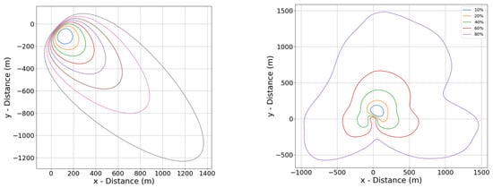
Figure 3.
Plots showing the single footprint in one half-hour instant (left) and footprint climatology (right) (measurement height 70 m) for July 2018.
The necessary input variables for the single-footprint calculation are measurement height above the displacement height (zm), roughness length (z0), mean wind speed at zm (umean), boundary layer height (h), Obukhov length (ol), standard deviation of lateral velocity fluctuations (sigmav) and friction velocity (ustar or u*). A uniform boundary layer height of 1000 m was applied across all datasets, aligning with the validated range reported by Kljun et al. [7]. Additional micrometeorological variables, such as the Obukhov length, wind direction, wind speed, roughness length, friction velocity, etc., were computed using the REddyProcWeb processing tool [26]. All parameters were obtained from the previously calculated fluxes or were specified according to the SMEAR Estonia’s eddy covariance equipment setup and the forest height data. The friction velocity (u*) was set more than or equal to 0.3 for the study to avoid the use of non-turbulent intervals for the footprint calculation [7,32], as previously used for the same measurements [28]. About 30% of the data were excluded due to low u* values, mostly occurring between 17:00 and 04:00 (nighttime). Wind from the northeast to east accounted for a slightly higher proportion of the low-turbulence cases, with no clear seasonal or monthly bias observed. All data analyses were performed in Python version 3.11.6 (Python Software Foundation, 2023).
2.5. Calculation of Peak Footprint Contribution
We calculated a single (two-dimensional flux) footprint function for each half-hourly flux dataset for all years from 2015 to 2020. Each single footprint can be seen as a signal transfer function that maps the source region for a single half-hourly integrated flux. For each flux data point, we get a different output, such as a structure array with the footprint (FFP) distribution, the downwind location of the footprint peak, a gridded array of crosswind-integrated footprint area and the gridded footprint function values of the crosswind-integrated footprint. However, in this study, we were interested in the maximum footprint contribution (the area of the highest contribution to the flux measured), which can be approximated by the peak location of the crosswind-integrated footprint function [7] in the downwind direction. The locations of footprint peaks with respect to the mast were calculated with the help of the wind direction information and the footprint functions’ distance information, as shown in Equations (3) and (4):
Then, the x and y coordinates were transformed to the Estonian Coordinate system of 1997 (EPSG:3301) so that they could be overlayed on the available base map layers in Geographic Information System software version 3.30.1. lmax represents the downwind distance from the measurement point to the location of the peak footprint contribution.
2.6. Cluster Analysis
Combining the half-hourly calculated peaks of the footprint function on a monthly basis revealed that depending on the wind direction, clusters of the EC flux signals were apparent (Figure 4). To determine spatially explicit areas that are dominating the flux signal, we used cluster algorithms specifically for spatial data. The hierarchical density-based spatial clustering of applications with noise (HDBSCAN) algorithm was employed for this analysis, utilizing the Python module ‘sklearn.cluster.HDBSCAN’ [33]. The HDBSCAN algorithm was selected because it is optimized for cluster recognition in large spatial datasets that include noise [34]. Using an unsupervised learning algorithm that evaluates the density of the points distributed in the footprint’s spatial domain let us process large quantities of data without having to provide prior estimates or parameters that, for instance, the k-means algorithm would require. Nevertheless, we conducted an assessment to determine the best match between the necessary hyperparameters of our data and the algorithm needs prior to its application to the large dataset. We determined the parameters, including the minimum number of points (min_samples) needed for a point to qualify as a core cluster point and neighborhood radius (ε epsilon). HDBSCAN performs DBSCAN over a range of ε values and integrates the results to identify clusters that maximize stability [35]. In this study, the values for minimum cluster size and min_samples were both set to 15 to ensure that the clusters were large enough to be meaningful while minimizing the formation of small, spurious clusters. The algorithm assigns numbers to the detected clusters starting from 0 in ascending order, while outliers are labeled as cluster −1. We note that the term “outlier” is somewhat misleading in the context of our data, but as it is used in the literature, we adopted it. Even though the term “outliers” may imply discarding them in the analyses, we treat them as points that do not belong to any cluster according to the distance definition used by HDBSCAN. The input data were scaled by applying the robust scaler procedure of the scikit-learn package [36] (with ‘StandardScaler’ applied in cases where a standard normalization was required).
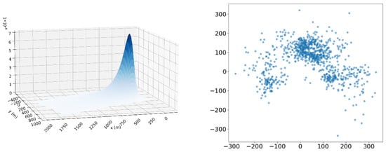
Figure 4.
Single footprint in three dimensions and points of maximum footprint contribution for July 2018. The coordinate origin (0,0) corresponds to the position of the measurement tower.
2.7. National Forest Inventory Dataset
The forest inventory dataset consists of information on land use information, information on road, ditch or track, area of the compartments, stand volume, proportion of tree species, soil type, site index, stand age, stand diameter, increment by year, stand volume, height and diameter by year. The dataset used in this study is available through the National Forest Register of Estonia (Metsaressursi arvestuse riiklik register, 2023) [https://register.metsad.ee/#/].
2.8. Merging Flux Footprint Data with Forest Inventory Data
To integrate the two datasets, spatial operations were performed using the open-source Python library GeoPandas [37]. The first dataset contained latitude and longitude coordinates representing footprint peak distances, along with associated micrometeorological data. The second dataset provided forestry information, including basal area, tree species composition and more. The forestry data were organized into a regular grid with a cell size of 12.5 × 12.5 m, as shown in Figure 5. In the first dataset, each peak distance was represented as a point with geographic coordinates. To align this with the forestry grid, each point was converted into a circular area centered on its respective coordinates. The radius of the circle was selected to approximate the area of a single forestry grid cell, ensuring a compatible spatial resolution between the two datasets.
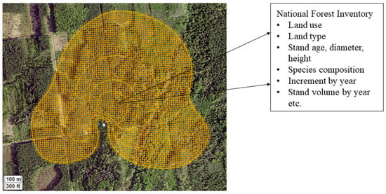
Figure 5.
Footprint climatology contours for July 2018 with 12.5 m × 12.5 m grids. The box showing the variables of the National Forest Inventory dataset. The white star represents the location of measurement tower. The map uses the EPSG:3301 (Estonian Coordinate System 1997) coordinate reference system. Shaded area indicates the flux footprint climatology for July 2018.
It is important to note that while peak distances are recorded as points, they represent only an approximate location of the signal’s origin and, as visible in Figure 3, cover an elliptic area. In practical terms, it is more accurate to consider an area surrounding each point as the likely source region. Therefore, the circular area was defined to correspond to the smallest available grid size (12.5 × 12.5 m), providing a reasonable basis for spatial comparison. By overlapping the outer boundaries of these peak-distance circles with the forestry grid, a spatial join was conducted. This operation associated each peak distance area, along with its micrometeorological data, with the corresponding forestry information. The resulting dataset combined footprint peak distance (location of maximum footprint contribution) information, eddy flux, micrometeorological measurements and forestry attributes, enabling further analysis.
3. Results
3.1. Overlaying the Clusters of Peak Footprint Contribution on Base Map
In order to reach a combined dataset of spatially explicit features and flux characteristics, the peak footprint clusters were superimposed onto the base map, which included quarters and compartments that denote different site types, utilizing the Quantum Geographic Information System (QGIS) version 3.30.1. This base map layer encompassed the footprint contribution area. The cluster data, comprising the X and Y coordinates of each peak footprint location, datetime, corresponding flux data and cluster ID for each footprint point, was incorporated into QGIS as a delimited text layer (Figure 6).
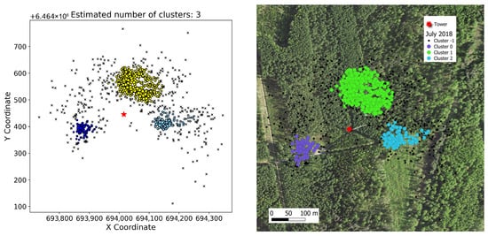
Figure 6.
Clusters obtained from the HDBSCAN cluster analysis (left), overlaid on the base map of the study site (right). The red star indicates the position of the measurement tower, and the map uses the EPSG:3301 (Estonian Coordinate System of 1997) coordinate reference system.
3.2. Results of Cluster Analysis
The number of clusters ranged from 2 (observed in several months) to 7 (January 2018 and February 2019). Outlier percentages varied between 11.7% (January 2019) and 58% (August 2017) (Figure 7). On average over the years, January exhibited the lowest proportion of outliers (20.65%), whereas August had the highest (42.65%). Details of the cluster characteristics are provided in Table A1.
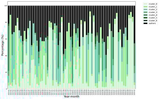
Figure 7.
Percentage of points in each cluster for all months from 2015 to 2020. Each color represents a different cluster, and black represents the outliers (Cluster −1).
Figure 8 illustrates wind direction patterns for August 2017 and January 2019, representing the months with the highest and lowest numbers of outliers, respectively. August shows a greater proportion of wind originating from heterogeneous directions, which likely contributed to the increased number of outliers observed during that period compared to the more uniform wind patterns in January.
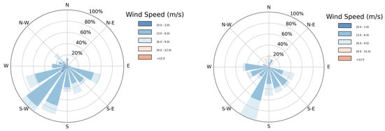
Figure 8.
Wind direction and wind speed for the months August 2017 (left) and January 2019 (right).
3.3. Species Composition by Cluster
One very interesting characteristic is the species composition within the footprint and the spatial distribution that can be revealed by the cluster analysis. Following the integration of flux data and forest inventory data, we were able to visualize these aspects of the forest ecosystem with respect to clusters obtained from the cluster analysis. Figure 9 shows the species composition by clusters on the left, and the wind rose on the right shows the related wind directions for July 2018. The bar graph shows the species composition percentage for each cluster, such that Pine is the dominating species in Clusters −1 (outliers), 0 and 1. However, in Cluster 2, Pine and Spruce made up almost the same share of the species composition.
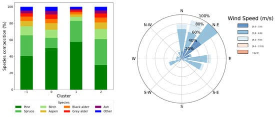
Figure 9.
Species composition of each cluster and wind rose showing the wind directions for July 2018.
Most of the wind in July 2018 blew from between north and east, with the highest frequency originating from the northeast. In contrast, winds were very sparse between the southwest and southeast, with no wind observed from the south. When analysing Figure 6, we can see that the wind direction and the cluster locations align, which is expected, since the wind direction coordinates are an input to the HDBSCAN algorithm.
3.4. Species Composition by Cluster with Wind Direction
Figure 10 gives a more detailed look at the species composition in the clusters than Figure 9. Here, the species composition is plotted against the wind direction, with breaks every 10 degrees. The proportion of Pine is 40–60% in Cluster 0 and slightly higher, 50–60%, in Cluster 1. Similarly, Pine and Spruce dominate Cluster 2, with Pine covering 20–40% and Spruce covering 20–60%. On the right, the plot shows the species composition for the outliers (those not belonging to any cluster). The species composition percentage in Cluster 2 is similar to that of other clusters; however, the gap between 160 and 220 degrees on the right-hand plot is due to the absence of wind from that direction, which can also be confirmed by the wind rose in Figure 9.
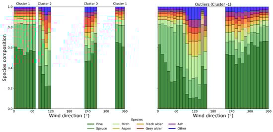
Figure 10.
Species composition with wind direction for each cluster for July 2018.
3.5. Species Composition and Cluster Dynamics (2015–2020)
Across the different years in July, three clusters were identified each year, except in 2017. These clusters were predominantly composed of conifer species, which accounted for approximately 30–80% of their composition (Figure 11a). However, the number of clusters in September across the years is more variable than in July. In 2016, 2019 and 2020, two clusters were identified, while 2018 had three clusters and 2015 and 2017 showed five and four clusters, respectively.
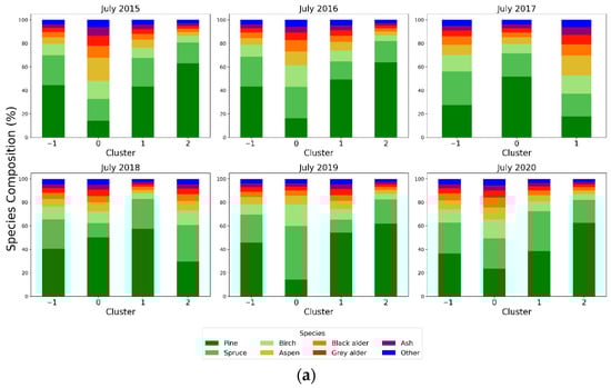
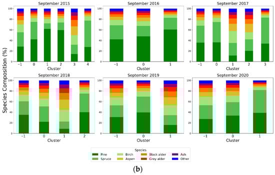
Figure 11.
Species composition by cluster (Cluster −1 represents the outlier group) for July (a) and September (b) from 2015 to 2020.
3.6. Spatiotemporal Data Usage and Feature Identification in QGIS
The merged dataset can be explored in multiple ways. Since we have monthly GeoJSON files, these can be used in, for instance, Python for feature visualization, data extraction and further analysis. The database we created allows us to implement, for instance, a microservice structure to enable machine-to-machine access and provide data for users via network and the possibility of automated access.
Alternatively, the data can be inspected interactively in QGIS for point-wise exploration. In Figure 12, each cluster is represented by differently colored points, while outliers are shown in black. The box highlights the features of the points within the cluster circled in red. A similar inspection can be carried out for any point, and the corresponding features can be easily retrieved.
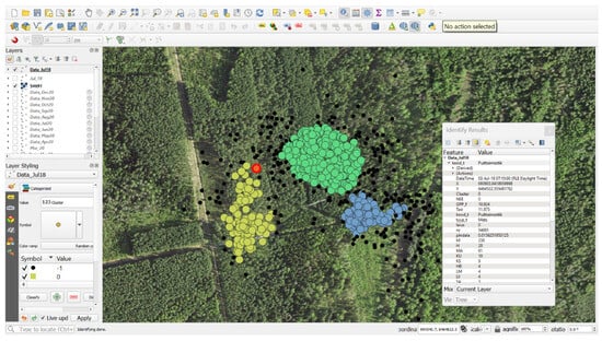
Figure 12.
Screenshot of the QGIS software, where the dataset is loaded as a delimited text file and each point is clickable to view its features. Each color represents a separate cluster, where black represents the outliers and the point highlighted with red is the selected point for exploration.
4. Discussions
The number of clusters identified each month ranged from 2 to 7 (Figure 7), mainly due to seasonal variations and changing wind conditions. The occurrence of a low number of clusters (2–3), and thereof one cluster containing a high number of points, occurs mostly during the autumn and winter months (October–January). In contrast, the number of clusters was mostly higher during the growing season (Appendix B) [38], making it more likely to observe greater variation in the characteristics of the underlying forest ecosystem when using the clusters. The observed variability in outlier percentages (see Table A1) may result from the combined influence of fluctuations in both wind direction and wind speed during the respective months.
The percentage weights of the detected clusters and outliers (Figure 7) can be used to assess the impact of an area on NEE:
Here, we can use a monthly aggregated NEE estimate as an example, and using Equation (5), the contribution of a spatial area—either by the clusters or the outliers—within the flux tower’s footprint can be calculated.
The spatial distribution of clusters and the number of outliers is influenced by the variability in wind direction, as shown in Figure 8 for August 2017 and January 2019. The greater heterogeneity in wind direction during August corresponds to a higher number of outliers. Similarly, species composition within clusters also varies from month to month.
In July 2018, species composition analysis showed that conifers dominated across all clusters (Figure 9). We interpret this result by comparing it with the overall reported species composition of drained peatland forests [39], where the coniferous fraction is approximately 30%. In contrast, the clusters contained between 60% and 80% of conifers. The dominance of Pine, followed by Spruce, aligns with known species distribution patterns. Among broadleaf species, Birch was dominant, consistent with its overall share reported in the literature.
Mapping the data of July 2018 using 10° bins (Figure 10) showed that clusters may exhibit a higher degree of homogeneity compared to outliers. This is expected, as outliers have a spatially wider distribution than the clusters. This enables the selection of different scenarios for assessing, for instance, carbon exchange associated with specific species distributions. It also makes it possible to detect clusters of approximately similar species contributions across the entire dataset.
The number of clusters in September across the years was more variable than in July. In 2016, 2019 and 2020, two clusters were identified, while 2018 had three clusters and 2015 and 2017 showed five and four clusters, respectively (Figure 11). This was an expected outcome, as the cluster selection algorithm was based on wind direction and wind speed data, which were different over the full annual cycle. The usual climatic conditions in Estonia include four distinct seasons, with spring and autumn typically showing greater variability than summer and winter due to the changes in sunlight. Despite these differences, the species composition remained comparable to July, with conifers (Pine and Spruce) accounting for between 20% and 80% of the cluster composition.
The consistent number of clusters observed in July compared to September (Figure 11) across different years indicates that increased wind pattern stability contributes to the emergence of spatial patterns in flux data. At sites like SMEAR Estonia, where the forest has a high degree of heterogeneity due to the management activities and the mosaic of changing soil conditions ranging from mineral to peatland soils, often on small spatial scales, the impact of clusters contributing to the overall flux to higher degree may introduce biases in the flux estimations. Chu et al. [40] discuss the influence of individual footprints at AmeriFlux sites, noting that they may introduce uncertainties while emphasizing the value of using single half-hourly footprints to capture fine-scale variability. At this stage, our clustering algorithm indicates that even the proposed use of footprint climatologies to reduce uncertainties [40] may still be influenced by dense single-footprint areas. Since our approach relies on peak single-footprint points, which capture the strongest contributions to flux estimates, future work should incorporate footprint climatologies and compare them with the aggregated flux estimates derived from the clusters.
By integrating eddy covariance fluxes, atmospheric concentrations and forest-related measurements, cluster information can be utilized to quantify NEE, GPP and RE at both site-specific and regional scales as well as for selected species groups. Such an approach offers a robust framework to support decision-making in carbon-smart forest management.
5. Conclusions
This study demonstrates the value of integrating high-frequency eddy covariance flux measurements with detailed forest inventory data to better understand the spatial and temporal dynamics of ecosystem–atmosphere exchanges in a heterogeneous hemiboreal forest. By applying a two-dimensional flux footprint model and unsupervised clustering algorithms, we were able to identify and map the dominant source areas contributing to measured fluxes at the SMEAR Estonia site. The overlay of these clusters with forest stand characteristics revealed clear links between flux patterns, wind direction and species composition, highlighting the influence of both biotic and abiotic factors on carbon and energy exchange.
The resulting merged dataset, structured at a fine spatial resolution (12.5 × 12.5 m2), enables spatially explicit analyses of forest growth and flux dynamics. Our approach allows for the detection of temporal changes in cluster patterns, the quantification of cluster contributions to net ecosystem exchange, and the assessment of how forest management and natural variability shape flux footprints. This framework provides a robust basis for future research on carbon cycling, supports the development of carbon-smart forest management strategies and offers a scalable methodology for other flux tower sites with heterogeneous landscapes.
Author Contributions
Conceptualization, A.T.M. and S.M.N.; methodology, A.T.M., D.K., A.P., E.G.F.M. and S.M.N.; project administration, S.M.N.; software, A.T.M., D.K., A.P., E.G.F.M. and S.M.N.; supervision, S.M.N.; writing—original draft, A.T.M.; writing—review and editing, A.T.M., D.K., A.P., E.G.F.M. and S.M.N. All authors have read and agreed to the published version of the manuscript.
Funding
This research was funded by the Estonian Research Council Grant PRG 1674 and the European Union’s Horizon 2020 Research and Innovation program (grant agreement no. 871115) ACTRIS IMP.
Data Availability Statement
The data will be made available upon request.
Acknowledgments
We acknowledge the Estonian Research Council Grant PRG 1674 and the European Union’s Horizon 2020 Research and Innovation program (grant agreement no. 871115) ACTRIS IMP.
Conflicts of Interest
The authors declare no conflicts of interest.
Abbreviations
The following abbreviations are used in this manuscript:
| FFP | Flux Footprint Prediction |
| HDBSCAN | Hierarchical Density-Based Spatial Clustering of Applications with Noise |
| NEE | Net Ecosystem Exchange |
| GPP | Gross Primary Productivity |
| RE | Respiration |
| EC | Eddy Covariance |
| QGIS | Quantum Geographic Information System |
| NFI | National Forest Inventory |
Appendix A

Table A1.
Result of HDBSCAN cluster analysis for years 2015–2020.
Table A1.
Result of HDBSCAN cluster analysis for years 2015–2020.
| Month | Metric | 2015 | 2016 | 2017 | 2018 | 2019 | 2020 |
|---|---|---|---|---|---|---|---|
| January | Num_Clusters | 6 | 3 | 2 | 7 | 3 | 2 |
| In_Cluster_Points | 752 (78.3%) | 582 (81.7%) | 907 (79.8%) | 742 (63.7%) | 885 (88.3%) | 1105 (84.3%) | |
| Outliers | 209 (21.7%) | 130 (18.3%) | 230 (20.2%) | 422 (36.3%) | 117 (11.7%) | 206 (15.7%) | |
| February | Num_Clusters | 2 | 4 | 4 | 3 | 7 | 2 |
| In_Cluster_Points | 461 (89.0%) | 597 (52.6%) | 598 (71.3%) | 579 (78.2%) | 736 (63.7%) | 1090 (91.2%) | |
| Outliers | 57 (11.0%) | 539 (47.4%) | 241 (28.7%) | 161 (21.8%) | 419 (36.3%) | 105 (8.8%) | |
| March | Num_Clusters | 4 | 3 | 3 | 4 | 6 | 4 |
| In_Cluster_Points | 691 (65.7%) | 621 (78.7%) | 753 (78.7%) | 722 (66.9%) | 865 (67.9%) | 677 (68.1%) | |
| Outliers | 360 (34.3%) | 168 (21.3%) | 204 (21.3%) | 358 (33.1%) | 409 (32.1%) | 317 (31.9%) | |
| April | Num_Clusters | 3 | 4 | 4 | 4 | 5 | 2 |
| In_Cluster_Points | 650 (68.2%) | 636 (67.2%) | 781 (76.2%) | 699 (72.7%) | 479 (55.4%) | 758 (71.4%) | |
| Outliers | 303 (31.8%) | 310 (32.8%) | 244 (23.8%) | 262 (27.3%) | 385 (44.6%) | 303 (28.6%) | |
| May | Num_Clusters | 2 | 4 | 5 | 3 | 2 | 4 |
| In_Cluster_Points | 610 (76.1%) | 470 (58.1%) | 501 (52.8%) | 455 (50.8%) | 695 (74.1%) | 528 (50.3%) | |
| Outliers | 192 (23.9%) | 339 (41.9%) | 448 (47.2%) | 440 (49.2%) | 243 (25.9%) | 521 (49.7%) | |
| June | Num_Clusters | 2 | 5 | 4 | 2 | 5 | 3 |
| In_Cluster_Points | 823 (85.2%) | 382 (44.8%) | 651 (67.8%) | 820 (82.7%) | 572 (60.5%) | 585 (66.3%) | |
| Outliers | 143 (14.8%) | 471 (55.2%) | 309 (32.2%) | 172 (17.3%) | 374 (39.5%) | 298 (33.7%) | |
| July | Num_Clusters | 3 | 3 | 2 | 3 | 3 | 3 |
| In_Cluster_Points | 624 (70.3%) | 612 (61.9%) | 737 (86.2%) | 586 (62.3%) | 500 (56.3%) | 665 (73.7%) | |
| Outliers | 263 (29.7%) | 377 (38.1%) | 118 (13.8%) | 354 (37.7%) | 388 (43.7%) | 237 (26.3%) | |
| August | Num_Clusters | 3 | 2 | 5 | 2 | 5 | 4 |
| In_Cluster_Points | 463 (63.8%) | 532 (57.4%) | 379 (42.0%) | 648 (81.1%) | 296 (40.9%) | 405 (58.8%) | |
| Outliers | 263 (36.2%) | 395 (42.6%) | 523 (58.0%) | 151 (18.9%) | 427 (59.1%) | 284 (41.2%) | |
| September | Num_Clusters | 5 | 2 | 4 | 3 | 2 | 2 |
| In_Cluster_Points | 430 (57.4%) | 461 (57.3%) | 416 (48.1%) | 580 (64.7%) | 548 (63.2%) | 924 (88.8%) | |
| Outliers | 319 (42.6%) | 344 (42.7%) | 448 (51.9%) | 317 (35.3%) | 319 (36.8%) | 117 (11.2%) | |
| October | Num_Clusters | 2 | 3 | 2 | 5 | 2 | 2 |
| In_Cluster_Points | 495 (69.7%) | 490 (61.6%) | 689 (69.1%) | 592 (67.3%) | 686 (78.6%) | 836 (92.4%) | |
| Outliers | 215 (30.3%) | 305 (38.4%) | 308 (30.9%) | 287 (32.7%) | 187 (21.4%) | 69 (7.6%) | |
| November | Num_Clusters | 4 | 6 | 2 | 2 | 4 | 2 |
| In_Cluster_Points | 628 (60.1%) | 463 (63.4%) | 820 (79.5%) | 920 (93.1%) | 707 (69.5%) | 967 (86.5%) | |
| Outliers | 417 (39.9%) | 267 (36.6%) | 212 (20.5%) | 68 (6.9%) | 310 (30.5%) | 151 (13.5%) | |
| December | Num_Clusters | 2 | 2 | 4 | 4 | 5 | 5 |
| In_Cluster_Points | 790 (72.8%) | 963 (81.5%) | 711 (62.6%) | 659 (66.4%) | 744 (62.4%) | 696 (54.7%) | |
| Outliers | 295 (27.2%) | 219 (18.5%) | 425 (37.4%) | 333 (33.6%) | 449 (37.6%) | 576 (45.3%) |
Appendix B. Ecosystem Exchange Variables
Figure A1 presents the daily averages of NEE, GPP and Respiration as calculated from the SMEAR Estonia tower footprint. The shaded gray area represents the range of these variables from 2015 to 2020, while the black line indicates their mean values over the same period. We observe an increase in gross primary production and respiration around the 100th day of the year, reaching and maintaining peak values, with some fluctuations, between approximately the 175th and 225th days, followed by a gradual decline. GPP approaches near zero around the 300th day of the year, while respiration reaches its minimum around the 340th day. Based on GPP onset and offset, the growing season length was estimated at approximately 200 days, which is consistent with the 204 days duration reported for Järvselja using the GDD5 approach [38]. We also observe that NEE turns negative just before day 100 and begins rising toward day 200, only becoming positive around day 250. The half-hourly flux data are the basis for the spatiotemporal dataset we aim to develop. To organize the input data so that we later can visualize the datasets in a meaningful way; therefore, we collected half-hourly data into monthly subsets for the whole 2015–2020 period.

Figure A1.
Annual representation of average net ecosystem exchange, gross primary production and ecosystem respiration from 2015 to 2020. The shaded area represents the range of measurements for the variables for the day of year, and the black line is the average of all years combined.
References
- Hari, P.; Andreae, M.O.; Kabat, P.; Kulmala, M. A Comprehensive Network of Measuring Stations to Monitor Climate Change. Boreal Environ. Res. 2009, 14, 442–446. [Google Scholar]
- Baldocchi, D.D. Assessing the Eddy Covariance Technique for Evaluating Carbon Dioxide Exchange Rates of Ecosystems: Past, Present and Future. Glob. Change Biol. 2003, 9, 479–492. [Google Scholar] [CrossRef]
- Baldocchi, D.D. How Eddy Covariance Flux Measurements Have Contributed to Our Understanding of Global Change Biology. Glob. Change Biol. 2020, 26, 242–260. [Google Scholar] [CrossRef]
- Hari, P.; Kulmala, M. Station for Measuring Ecosystem-Atmosphere Relations (SMEAR II). Boreal Environ. Res. 2005, 10, 315–322. [Google Scholar]
- Noe, S.M.; Niinemets, Ü.; Krasnova, A.; Krasnov, D.; Motallebi, A.; Kängsepp, V.; Jõgiste, K.; Hõrrak, U.; Komsaare, K.; Mirme, S.; et al. SMEAR Estonia: Perspectives of a Large-Scale Forest Ecosystem–Atmosphere Research Infrastructure. For. Stud. 2015, 63, 56–84. [Google Scholar] [CrossRef]
- Baldocchi, D. Measuring Fluxes of Trace Gases and Energy between Ecosystems and the Atmosphere–the State and Future of the Eddy Covariance Method. Glob. Change Biol. 2014, 20, 3600–3609. [Google Scholar] [CrossRef]
- Kljun, N.; Calanca, P.; Rotach, M.W.; Schmid, H.P. A Simple Two-Dimensional Parameterisation for Flux Footprint Prediction (FFP). Geosci. Model Dev. 2015, 8, 3695–3713. [Google Scholar] [CrossRef]
- Running, S.W.; Baldocchi, D.D.; Turner, D.P.; Gower, S.T.; Bakwin, P.S.; Hibbard, K.A. A Global Terrestrial Monitoring Network Integrating Tower Fluxes, Flask Sampling, Ecosystem Modeling and EOS Satellite Data. Remote Sens. Environ. 1999, 70, 108–127. [Google Scholar] [CrossRef]
- Burba, G. Eddy Covariance Method: For Scientific, Regulatory, and Commercial Applications; Updated and Expanded 2022 Edition; LI-COR Biosciences: Lincoln, NE, USA, 2022; ISBN 978-0-578-97714-0. [Google Scholar]
- Yu, M.; Wu, B.; Zeng, H.; Xing, Q.; Zhu, W. The Impacts of Vegetation and Meteorological Factors on Aerodynamic Roughness Length at Different Time Scales. Atmosphere 2018, 9, 149. [Google Scholar] [CrossRef]
- Schmid, H.P. Footprint Modeling for Vegetation Atmosphere Exchange Studies: A Review and Perspective. Agric. For. Meteorol. 2002, 113, 159–183. [Google Scholar] [CrossRef]
- Vesala, T.; Kljun, N.; Rannik, Ü.; Rinne, J.; Sogachev, A.; Markkanen, T.; Sabelfeld, K.; Foken, T.; Leclerc, M.Y. Flux and Concentration Footprint Modelling: State of the Art. Environ. Pollut. 2008, 152, 653–666. [Google Scholar] [CrossRef] [PubMed]
- Kormann, R.; Meixner, F.X. An Analytical Footprint Model For Non-Neutral Stratification. Bound.-Layer Meteorol. 2001, 99, 207–224. [Google Scholar] [CrossRef]
- Kollo, J.; Padari, A.; Krasnova, A.; Kangur, A.; Noe, S.M. Development of a Footprint Description Tool Utilizing SMEAR Estonia Eddy-Covariance Data and Footprint Modelling in Combination with Remote Sensed Forest Species and Land Cover Data. For. Stud. 2023, 79, 90–104. [Google Scholar] [CrossRef]
- Kangur, A.; Nigul, K.; Padari, A.; Kiviste, A.; Korjus, H.; Laarmann, D.; Põldveer, E.; Mitt, R.; Frelich, L.E.; Jõgiste, K.; et al. Composition of Live, Dead and Downed Trees in Järvselja Old-Growth Forest. For. Stud. 2021, 75, 15–40. [Google Scholar] [CrossRef]
- Kohava, P. Forests in Estonia 1999 (Eesti Metsad 1999); OÜ Eesti Metsakorralduskeskus: Tallinn, Estonia, 2000. [Google Scholar]
- Lang, M.; Sims, A.; Pärna, K.; Kangro, R.; Möls, M.; Mõistus, M.; Kiviste, A.; Tee, M.; Vajakas, T.; Rennel, M. Remote-Sensing Support for the Estonian National Forest Inventory, Facilitating the Construction of Maps for Forest Height, Standing-Wood Volume, and Tree Species Composition. For. Stud. 2020, 73, 77–97. [Google Scholar] [CrossRef]
- Omoniyi, T.O.; Sims, A. Enhancing the Precision of Forest Growing Stock Volume in the Estonian National Forest Inventory with Different Predictive Techniques and Remote Sensing Data. Remote Sens. 2024, 16, 3794. [Google Scholar] [CrossRef]
- Babst, F.; Bouriaud, O.; Papale, D.; Gielen, B.; Janssens, I.A.; Nikinmaa, E.; Ibrom, A.; Wu, J.; Bernhofer, C.; Köstner, B.; et al. Above-ground Woody Carbon Sequestration Measured from Tree Rings Is Coherent with Net Ecosystem Productivity at Five Eddy-covariance Sites. New Phytol. 2014, 201, 1289–1303. [Google Scholar] [CrossRef]
- Ferster, C.J.; Trofymow, J.; Coops, N.C.; Chen, B.; Black, T.A. Comparison of Carbon-Stock Changes, Eddy-Covariance Carbon Fluxes and Model Estimates in Coastal Douglas-Fir Stands in British Columbia. For. Ecosyst. 2015, 2, 13. [Google Scholar] [CrossRef]
- Giannico, V.; Chen, J.; Shao, C.; Ouyang, Z.; John, R.; Lafortezza, R. Contributions of Landscape Heterogeneity within the Footprint of Eddy-Covariance Towers to Flux Measurements. Agric. For. Meteorol. 2018, 260–261, 144–153. [Google Scholar] [CrossRef]
- Griebel, A.; Bennett, L.T.; Metzen, D.; Cleverly, J.; Burba, G.; Arndt, S.K. Effects of Inhomogeneities within the Flux Footprint on the Interpretation of Seasonal, Annual, and Interannual Ecosystem Carbon Exchange. Agric. For. Meteorol. 2016, 221, 50–60. [Google Scholar] [CrossRef]
- Wang, H.; Jia, G.; Zhang, A.; Miao, C. Assessment of Spatial Representativeness of Eddy Covariance Flux Data from Flux Tower to Regional Grid. Remote Sens. 2016, 8, 742. [Google Scholar] [CrossRef]
- Coates, T.W.; Flesch, T.K.; McGinn, S.M.; Charmley, E.; Chen, D. Evaluating an Eddy Covariance Technique to Estimate Point-Source Emissions and Its Potential Application to Grazing Cattle. Agric. For. Meteorol. 2017, 234–235, 164–171. [Google Scholar] [CrossRef]
- Ahti, T.; Hämet-Ahti, L.; Jalas, J. Vegetation Zones and Their Sections in Northwestern Europe. Ann. Bot. Fenn. 1968, 5, 169–211. [Google Scholar]
- Wutzler, T.; Lucas-Moffat, A.; Migliavacca, M.; Knauer, J.; Sickel, K.; Šigut, L.; Menzer, O.; Reichstein, M. Basic and Extensible Post-Processing of Eddy Covariance Flux Data with REddyProc. Biogeosciences 2018, 15, 5015–5030. [Google Scholar] [CrossRef]
- Baldocchi, D.D.; Hincks, B.B.; Meyers, T.P. Measuring Biosphere-Atmosphere Exchanges of Biologically Related Gases with Micrometeorological Methods. Ecology 1988, 69, 1331–1340. [Google Scholar] [CrossRef]
- Krasnova, A.; Mander, Ü.; Noe, S.M.; Uri, V.; Krasnov, D.; Soosaar, K. Hemiboreal Forests’ CO2 Fluxes Response to the European 2018 Heatwave. Agric. For. Meteorol. 2022, 323, 109042. [Google Scholar] [CrossRef]
- Krasnova, A.; Kukumägi, M.; Mander, Ü.; Torga, R.; Krasnov, D.; Noe, S.M.; Ostonen, I.; Püttsepp, Ü.; Killian, H.; Uri, V.; et al. Carbon Exchange in a Hemiboreal Mixed Forest in Relation to Tree Species Composition. Agric. For. Meteorol. 2019, 275, 11–23. [Google Scholar] [CrossRef]
- Reichstein, M.; Falge, E.; Baldocchi, D.; Papale, D.; Aubinet, M.; Berbigier, P.; Bernhofer, C.; Buchmann, N.; Gilmanov, T.; Granier, A.; et al. On the Separation of Net Ecosystem Exchange into Assimilation and Ecosystem Respiration: Review and Improved Algorithm. Glob. Change Biol. 2005, 11, 1424–1439. [Google Scholar] [CrossRef]
- Gong, H.; Wang, Y.; Wang, G.; Gao, Y.; Li, G.; Kuang, Z.; Zhuo, X.; Bi, J.; Wang, P.; Wang, W.; et al. Quantifying the Spatial Representativeness of Carbon Flux Footprints of a Grassland Ecosystem in the Semi-Arid Region. JGR Atmos. 2023, 128, e2022JD038269. [Google Scholar] [CrossRef]
- Mammarella, I.; Kolari, P.; Rinne, J.; Keronen, P.; Pumpanen, J.; Vesala, T. Determining the Contribution of Vertical Advection to the Net Ecosystem Exchange at Hyytiälä Forest, Finland. Tellus B Chem. Phys. Meteorol. 2007, 59, 900. [Google Scholar] [CrossRef]
- McInnes, L.; Healy, J. Accelerated Hierarchical Density Based Clustering. In Proceedings of the 2017 IEEE International Conference on Data Mining Workshops (ICDMW), New Orleans, LA, USA, 18–21 November 2017; pp. 33–42. [Google Scholar]
- Campello, R.J.G.B.; Moulavi, D.; Sander, J. Density-Based Clustering Based on Hierarchical Density Estimates. In Advances in Knowledge Discovery and Data Mining; Pei, J., Tseng, V.S., Cao, L., Motoda, H., Xu, G., Eds.; Lecture Notes in Computer Science; Springer: Berlin/Heidelberg, Germany, 2013; Volume 7819, pp. 160–172. ISBN 978-3-642-37455-5. [Google Scholar]
- McInnes, L.; Healy, J.; Astels, S. Hdbscan: Hierarchical Density Based Clustering. J. Open Source Softw. 2017, 2, 205. [Google Scholar] [CrossRef]
- Pedregosa, F.; Varoquaux, G.; Gramfort, A.; Michel, V.; Thirion, B.; Grisel, O.; Blondel, M.; Prettenhofer, P.; Weiss, R.; Dubourg, V.; et al. Scikit-Learn: Machine Learning in Python. J. Mach. Learn. Res. 2011, 12, 2825–2830. [Google Scholar]
- Jordahl, K.; den Bossche, J.V.; Fleischmann, M.; Wasserman, J.; McBride, J.; Gerard, J.; Tratner, J.; Perry, M.; Badaracco, A.G.; Farmer, C.; et al. Geopandas/Geopandas: V0.8.1; Zenodo: Genève, Switzerland, 2020. [Google Scholar]
- Kollo, J.; Metslaid, S.; Padari, A.; Hordo, M.; Kangur, A.; Noe, S.M. Trends in Thermal Growing Season Length from Years 1955–2020—A Case Study in Hemiboreal Forest in Estonia. Boreal Environ. Res. 2023, 28, 169–180. [Google Scholar]
- Sirkas, F.; Valgepea, M. (Eds.) Aastaraamat Mets 2023 (Yearbook Forest 2023); Keskkonnaagentuur: Tallinn, Estonia, 2025. [Google Scholar]
- Chu, H.; Luo, X.; Ouyang, Z.; Chan, W.S.; Dengel, S.; Biraud, S.C.; Torn, M.S.; Metzger, S.; Kumar, J.; Arain, M.A.; et al. Representativeness of Eddy-Covariance Flux Footprints for Areas Surrounding AmeriFlux Sites. Agric. For. Meteorol. 2021, 301–302, 108350. [Google Scholar] [CrossRef]
Disclaimer/Publisher’s Note: The statements, opinions and data contained in all publications are solely those of the individual author(s) and contributor(s) and not of MDPI and/or the editor(s). MDPI and/or the editor(s) disclaim responsibility for any injury to people or property resulting from any ideas, methods, instructions or products referred to in the content. |
© 2025 by the authors. Licensee MDPI, Basel, Switzerland. This article is an open access article distributed under the terms and conditions of the Creative Commons Attribution (CC BY) license (https://creativecommons.org/licenses/by/4.0/).