Experimental–Numerical Investigation of Natural Convection from a Plate Fin Heat Sink with Correlation Assessment

Abstract

This study investigates the thermal performance of a passive vertical aluminum heat sink with plate fins through combined experimental measurements and numerical simulations. Using a custom-made experimental apparatus which used water as the heat source, heat transfer rate was determined, and heat transfer coefficient was compared against established empirical correlations, demonstrating good agreement. A 3D steady-state mathematical model was developed to capture the conjugate heat transfer problem of conduction and natural convection, with buoyancy-driven airflow modeled with the incompressible ideal gas law. The problem was solved numerically using the finite volume method through ANSYS Fluent 18.2 solver and validated against experimental data and analytical correlations, exhibiting good agreement throughout. Parametric analysis followed, investigating the influence of various base (50, 65, 80 °C) and ambient (19, 24, 29 °C) temperatures, resulting in base-to-ambient temperature differences from 21 to 61 °C. Increasing this temperature difference led to a significant increase in heat transfer rate, while heat transfer coefficient increased and overall thermal resistance decreased moderately. Additionally, a Nusselt–Rayleigh (Nu–Ra) number correlation, consistent with ranges reported in the literature, was derived, providing the scaling to predict the thermal performance of similar natural convection-governed heat sinks. The validated computational methodology, combined with obtained experimental and numerical results, presents a foundation for future studies focused on more complex heat sink geometries and physics.

1. Introduction

Since Gordon Moore’s 1965 prediction that transistor density would double approximately every two years, the thermal load of electronic devices has risen steadily. While computational performance has surged, the ability to remove waste heat without performance degradation has emerged as a key limiting factor. In high-power electronics, lighting systems, and renewable energy converters, thermal management is not only a matter of efficiency, but also a key factor in component reliability, operational lifespan, and safety [1]. Heat sinks operate by transferring heat from a solid surface to the surrounding fluid, often air, through a combination of conduction within the solid, convection between the solid and fluid, and radiation to the surroundings, with the intensity of the latter depending on the emissivity of the surface. They can be classified by cooling mode, being split into passive, active, and hybrid types. Active heat sinks use forced convection, typically via fans or blowers, to increase heat transfer rates, and are common in high-density electronics such as CPUs and telecommunications equipment [2]. Passive heat sinks rely solely on natural convection and radiation, making them ideal for applications requiring silence, low maintenance, and high reliability, such as LED lighting, photovoltaic inverters, and certain aerospace systems [3].

Plate fin heat sinks are widely used for their predictable performance and ease of manufacture, while pin fin arrangements [4] can provide more isotropic cooling in multidirectional flow environments. More complex geometries, such as wavy fins [5], rippling fins [6], louvered fins [7], and porous metal foams [8], have been explored to disrupt boundary layers and enhance convection. Vertical orientation promotes stable airflow and plume formation, while horizontal or inclined arrangements typically reduce heat transfer rates [9].

Early theoretical treatments of natural convection in vertical fin arrays date back to the work of Elenbaas [10] in the mid-20th century, but the formulations and guidelines provided by Bar-Cohen and Rohsenow [11] remain foundational in modern heat sink considerations. Their semi-analytical model provided a framework for predicting thermally optimal fin spacing in passive heat sinks, balancing conductive and convective resistances. In addition to analytical and semi-analytical treatments, passive heat sinks have been investigated through both experiments and numerical simulations.

Ahmadi et al. [12] performed an experimental and numerical investigation of steady-state natural convection from vertical rectangular interrupted fins. After observing that interruptions greatly influence thermal performance, they provided a correlation for determining the optimum interruption length.

Quintino et al. [13] numerically studied buoyancy-driven convection from staggered heated vertical plates in air using a SIMPLE-C solver. Varying Rayleigh number, normalized spacing, and vertical misalignment, they found an optimal separation that maximizes heat transfer and depends on Ra and alignment, and derived dimensionless correlations for plates and arrays.

Shen et al. [14] conducted an experimental and CFD study of rectangular plate fin heat sinks on LEDs across eight orientations, observing that orientation and fin spacing are the significant operating parameters. They provided simple Nusselt–Rayleigh (Nu–Ra) correlations for several inclined cases across a range of operating temperatures.

Fuse et al. [15] included both base and ambient temperature variation in their experiments, providing valuable validation data for CFD models and demonstrating that changes in ambient temperature can significantly shift optimal design points.

Dewilde et al. [16] conducted an extensive 2D and quasi-3D CFD analysis of natural convection plate fin heat sinks spanning a wide range of Rayleigh, Grashof, and Elenbaas numbers, comparing laminar and turbulence models and offering mesh refinement guidelines tailored to buoyancy-driven flows. They found that the quasi-3D model with transition-SST performed best but modestly overestimated the heat flux. The authors also observed that several classical correlations can deviate and often underestimate Nu once transitional or turbulent flow appears, i.e., at high Ra.

Lee et al. [17] experimentally proposed a correlation for Nusselt number for enhancing the thermal efficiency of a cylindrical heat sink with perpendicularly oriented triangular fins under natural convection. Their study included different fin numbers, different fin heights, and varied base temperatures. They found that the correlation was suitable for the Rayleigh number range between 10³ and 1.2 × 10⁵.

Rao and Somkuwar [18] investigated heat dissipation through a heat sink with tapered fin heat sink. Varying taper between 1 and 3° under different thermal loads, they found that an inclination of approximately 2° minimized thermal resistance and maximized heat transfer coefficient among the tested geometries.

Joo and Kim [19] analytically compared and optimized plate fin and pin fin heat sinks in natural convection with a vertical base. They proposed and experimentally validated a new heat transfer coefficient correlation for pin fins, then optimized both designs under equal base-to-ambient temperature difference, base size, and fin height. They observed that plate fins maximize total heat dissipation, while pin fins maximize heat per unit mass.

Huang et al. [20] analyzed natural convection behavior of a heat pipe heat sink with a plate fin array of variable height using 3D CFD and multi-objective optimization. With the heat sink operating under still air, fin height distributions were varied to reduce flow resistance and improve thermal performance relative to uniform fins.

As seen from the overview, one of the most practical outcomes of both experimental and numerical studies is the derivation of Nu–Ra correlations, which provide compact predictive relationships for convective performance. The classical form, Nu = C·Raⁿ, is widely used but often requires geometry-specific constants and exponents. While substantial progress has been made in modeling, testing, and correlating the performance of passive heat sinks, relatively few studies integrate a numerical framework with systematic variation of both base and ambient temperatures. Even fewer derive generalized Nu–Ra correlations that explicitly account for temperature-dependent air properties in their considerations.

Addressing this gap, the present work develops an experimentally validated CFD model using the incompressible ideal gas formulation for density, evaluates performance over a range of operating temperatures, and proposes a Nu–Ra correlation applicable to similar geometries and conditions. The novelty lies in delivering a validation quality reference that simultaneously reconciles the calorimetry-based heat transfer rate and the average heat transfer coefficient with fin and base temperature distribution, as well as employing a 3D model that resolves finite array end effects, fin tip exchange, and lateral bypass absent in 2D idealizations. The geometry and boundary conditions needed to enable reproducibility and benchmarking are fully documented. Additionally, the compact Nu–Ra scaling with explicit bounds for the tested geometry and operating range is reported to enable rapid sizing and preliminary design screening of similar plate fin heat sinks under natural convection. This integrated experiment–model dataset serves as a practical reference for designers working in passive, power-free cooling.

2. Physical Model

The heat sink analyzed in the present study is a commercially available extruded aluminum unit with straight, vertical plate fins (Figure 1). No additional surface treatment was applied, so all surfaces are bare aluminum. Geometrically, the heat sink has an overall width (W) of 123 mm. A planar base with a thickness (t_b) of 6 mm supports an array of 11 identical fins (N) with a length (L) of 100 mm, which is equal to the overall length. Each fin is rectangular, with a thickness (t_f) of 3 mm and height (H), i.e., perpendicular distance from the base, of 30 mm. Fin spacing (s) is 9 mm. These dimensions were used in subsequent experimental and numerical investigations.

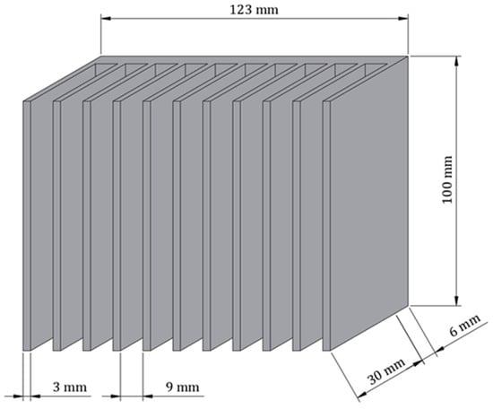
Figure 1. Schematic of the passive heat sink analyzed in the present study with indicated dimensions.

3. Experimental Setup and Procedure

3.1. Experimental Methodology

A calorimetric experiment was conducted to assess the heat sink thermal performance. Water was used as the internal heat source to enable straightforward sensible heat calorimetry: integrating the time history of the bulk temperature yields a direct, low-uncertainty estimate of the exchanged thermal energy and the corresponding heat transfer rate for validation. The use of other heat sources (e.g., phase change materials) instead of water, while facilitating near-isothermal energy release, would complicate energy accounting (by introducing latent heat, moving phase front, and subcooling/hysteresis) and increase the uncertainty in estimating the thermal energy exchanged. The heat sink was mounted and fixed onto the vessel, and the heat sink base was coated with a thin, uniform layer of silicone thermal paste before mounting to ensure low thermal contact resistance. To prevent heat dissipation to the environment, every face of the vessel (except the one in contact with the heat sink) was insulated with 25 mm of expanded rubber foam and covered in aluminum foil [21].

Four K-type thermocouples, with declared accuracies of ±0.2 °C, were placed along the width and length of a representative inner fin surface in order to monitor time-wise temperature changes at various characteristic positions. Thermocouples TC1 and TC2 were placed mid-length along the fin height, 1 and 15 mm from the heat sink base surface, respectively. Thermocouples TC3 and TC4 were placed near the edge of the fin in the height direction, 29 mm from the heat sink base surface, at the bottom and top positions along the length, at 1 and 99 mm from the bottom of the fin. An additional thermocouple was placed at the junction between the vessel and the heat sink base to obtain the heat sink base temperature (TCb). Water bulk temperature inside the vessel (T_w) and ambient air temperature (T_a) were measured using thermistor probes, with declared accuracies of ±0.02 °C. Temperatures were logged every second using a data logger and stored in computer memory. A schematic with thermocouple positions is given in Figure 2, while Figure 3 depicts the assembled experimental setup.

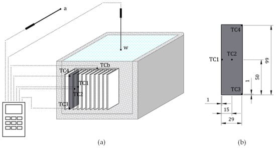
Figure 2. Schematic of the experimental setup (a) and placement of thermocouples on the fin (TC1–TC4) with reference offsets ((b); mm).

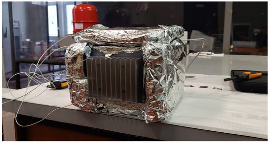
Figure 3. Assembled experimental setup.

The experiment, i.e., temperature sampling, began once water at the uniform temperature was poured into the vessel. After the initial unsteady phase, where both the vessel and heat sink temperatures increase as a result of heat transfer from the water, and water bulk temperature decreases rapidly as a result, the heat sink reached its operating temperature, i.e., steady-state set in, where water temperatures decreased more steadily and heat sink surface temperatures exhibited very little variation. This state was observed for 16 min, after which the experiment was discontinued.

3.2. Uncertainty in Thermal Energy Input

Thermal energy Q transferred from the water vessel to the aluminum heat sink during the steady-state interval was calculated as

$$Q=m_{\mathrm{w}}{c}_{\mathrm{w}}\mathsf{\Delta }{T}_{\mathrm{w}}$$

(1)

where m_w is the mass of water, c_w is its specific heat capacity, and ΔT_w is the measured temperature drop during the observed steady-state period. In the present experiments, m_w = 3.467 kg (balance uncertainty u_mw = 0.005 kg), c_w = 4184 J/(kg·K) (standard uncertainty u_cw = 2.09 J/(kg·K)) and ΔT_w = 0.61 K (u_ΔTw = 0.02 K). Inputting the values of m_w, c_w, and ΔT_w into Equation (1) gives Q = 8848.6 J.

To quantify the uncertainty in Q, the root-sum-square propagation of the individual uncertainties was obtained according to Moffat [22]. The sensitivity coefficients are defined as:

$$S_{\mathrm{m}}={\displaystyle \frac{\mathsf{\partial }Q}{\mathsf{\partial }m}}=c_{\mathrm{w}}\mathsf{\Delta }{T}_{\mathrm{w}}$$

(2)

$$S_{\mathrm{c}\mathrm{w}}={\displaystyle \frac{\mathsf{\partial }Q}{\mathsf{\partial }{c}_{\mathrm{w}}}}=m\mathsf{\Delta }{T}_{\mathrm{w}}$$

(3)

$$S_{\mathsf{\Delta }\mathrm{T}\mathrm{w}}={\displaystyle \frac{\mathsf{\partial }Q}{\mathsf{\partial }\mathsf{\Delta }{T}_{\mathrm{w}}}}=m_{\mathrm{w}}{c}_{\mathrm{w}}$$

(4)

The combined standard uncertainty u_Q is calculated as

$$u_{\mathrm{Q}}=\sqrt{{\left(S_{\mathrm{m}\mathrm{w}}{u}_{\mathrm{m}\mathrm{w}}\right)}^2+{\left(S_{\mathrm{c}\mathrm{w}}{u}_{\mathrm{c}\mathrm{w}}\right)}^2+{\left(S_{\mathsf{\Delta }\mathrm{T}\mathrm{w}}{u}_{\mathsf{\Delta }\mathrm{T}\mathrm{w}}\right)}^2}$$

(5)

Inputting corresponding calculated values of S_m, S_cw, and S_ΔTw into Equation (5) results in the combined standard uncertainty of 290.4 J or relative uncertainty of 3.28% for obtained Q. Because the average heat transfer rate and both specific heat fluxes are derived from the same thermal energy, their relative standard uncertainties are identical to that of Q.

4. Experimental Results

The total experiment ran for 28 min. For the first 12 min, thermocouples at the heat sink positions showed an increase in temperature, but after that, steady-state set in, and it was kept for t = 16 min (960 s). Throughout that time, bulk water temperature had been gradually decreasing. At the start and the end of the steady-state period, bulk water temperature was read, standing at T_w,start = 52.82 and T_w,end = 52.21 °C, respectively. In the same interval, the heat sink base temperature decreased by 0.4 °C, going from 50.2 to 49.8 °C, averaging to 50 °C throughout the interval. Heat sink surface temperatures exhibited even less variation in the same period, up to 0.3 °C. Temperature profiles of water (w) and air (a), as well as the heat sink base (TCb) and surface (TC1, TC2, TC3, TC4) throughout the measurement period and their averaged steady-state readings, are given in Figure 4 and Table 1, respectively.

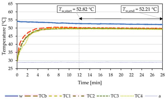
Figure 4. Temperature profiles of water, air, and heat sink base and surface for the performed measurement.

Table 1. Thermocouple designations and their corresponding steady-state readings.

Temperature Sensor	Steady-State Reading [°C]
TCb	50
TC1	49.8
TC2	49.7
TC3	49.4
TC4	49.6
Tb	50
w	52.82–52.21
a	29.02

From the obtained steady-state temperatures at different positions on the characteristic fin, it can be observed that the highest recorded temperatures, TC1 and TC2, are located closest to the base junction, i.e., closest to the heat source. The temperature drop increases as the position moves away from the heat source, at positions TC3 and TC4. At position TC3, located at the bottom of the fin and near the tip, the incoming air is at ambient temperature and has a thinner boundary layer, so it removes heat more intensely, making position TC3 the coolest examined position. As the buoyant air warms and the boundary layer thickens while it rises, local heat transfer coefficients drop. As a result, at the top of the fin, position TC4, the temperature is slightly higher than at the equivalent position at the bottom.

Heat transfer rate ($\dot{Q}$) between the water and the heat sink base equals the one between the heat sink surface and the ambient, and is calculated by dividing Q of 8848.6 J by the time of 960 s, resulting in $\dot{Q}$ = 9.22 W.

Due to the very low emissivity of the aluminum surface of the heat sink, it can be estimated that radiation contributes to approximately 5% or less in the overall heat transfer from the heat sink [23]. Therefore, for the simplicity of the investigation, it is assumed that heat dissipation from the heat sink occurs only via natural convection.

In order to obtain specific heat fluxes on the base surface area and on the ambient side, their surface areas need to be defined:

$$A_b=WL$$

(6)

$$A_s=2NHL+2NH{t}_f+NL{t}_f+2L{t}_{\mathrm{b}}+2W{t}_{\mathrm{b}}+\left(N-1\right)Ls$$

(7)

When corresponding values of geometry parameters are input in Equations (6) and (7), base surface area is 0.0123 m², while heat sink surface area on the ambient side is 0.082 m². Specific heat fluxes at the heat sink base (${\dot{q}}_{\mathrm{b}}$) and at the heat sink surface (${\dot{q}}_{\mathrm{s}}$) can be calculated by dividing the heat transfer rate by their respective surface areas, resulting in ${\dot{q}}_{\mathrm{b}}$ = 749.37 W/m² and ${\dot{q}}_{\mathrm{s}}$ = 112.63 W/m².

Heat transfer coefficient h is obtained by dividing the specific heat flux at the heat sink surface by the temperature difference between the average temperature on the heat sink surface (T_s) and the temperature of the ambient air (T_a). Temperature T_s is calculated as the average between the characteristic fin surface steady-state temperatures collected from thermocouples TC1, TC2, TC3, and TC4:

$$T_{\mathrm{s}}={\displaystyle \frac{1}{4}}\sum _{i=1}^4{T}_{\mathrm{T}\mathrm{C}i}$$

(8)

The experimentally determined heat transfer coefficient can be evaluated through comparison against two established correlations. The correlations provide empirical expressions as a means to obtain the dimensionless Nusselt number (Nu) and often contain other dimensionless parameters. These dimensionless parameters depend on geometry and thermophysical properties, which are evaluated at the film temperature, which is calculated as the arithmetic mean of the surface temperature and the free stream (ambient) fluid temperature. The list of thermophysical properties, taken at the film temperature of 40 °C, are given in Table 2.

Table 2. Thermophysical properties of air at film temperature.

Thermophysical Property	Value
Thermal expansion coefficient, βa [1/K]	0.0032
Density, ρa [kg/m3]	1.13
Thermal conductivity, ka [W/(m·K)]	0.0267
Specific heat capacity, cp,a [J/(kg·K)]	1007
Dynamic viscosity, μa [Pa∙s]	1.872 × 10−5

The correlation for a vertical isothermal plate proposed by Churchill and Chu [24] expresses the average Nusselt number as:

$${\mathrm{N}\mathrm{u}}_{\mathrm{L}}={\left\{0.825+{\displaystyle \frac{0.387{\mathrm{R}\mathrm{a}}_L^{1/6}}{{\left[1+{\left(0.492/\mathrm{P}\mathrm{r}\right)}^{\frac{9}{16}}\right]}^{8/27}}}\right\}}^2$$

(9)

In the expression, Ra_L is the Rayleigh number based on the fin length L, while Pr is the Prandtl number:

$${\mathrm{R}\mathrm{a}}_L={\displaystyle \frac{g{\beta }_{\mathrm{a}}{\rho }_{\mathrm{a}}^2{c}_{\mathrm{p},\mathrm{a}}\left(T_s-T_a\right)L^3}{{\mu }_{\mathrm{a}}{k}_{\mathrm{a}}}}$$

(10)

$$\mathrm{P}\mathrm{r}={\displaystyle \frac{{\mu }_{\mathrm{a}}{c}_{\mathrm{p},\mathrm{a}}}{k_{\mathrm{a}}}}$$

(11)

Recognizing that the considered heat sink is a finned surface, i.e., a collection of plates, rather than a single plate, the correlation for symmetric isothermal plates, assembled by Bar-Cohen and Rohsenow [11], has also been examined:

$${\mathrm{N}\mathrm{u}}_{\mathrm{s}}={\left[{\displaystyle \frac{576}{{\left(R{a}_{\mathrm{s}}s/L\right)}^2}}+{\displaystyle \frac{2.873}{{\left(R{a}_{\mathrm{s}}s/L\right)}^{0.5}}}\right]}^{-0.5}$$

(12)

In their formulation, the Rayleigh number is based on the fin spacing s, with the relation between Ra_s and Ra_L defined as $R{a}_{\mathrm{s}}=R{a}_{\mathrm{L}}{\displaystyle \frac{s^3}{L^3}}$.

Calculated values of Ra_L, Pr, Nu_L, Ra_s, and Nu_s, necessary for the calculation of correlation-based heat transfer coefficients, are provided in Table 3.

Table 3. Values of dimensionless parameters used in the correlations.

Dimensionless Parameter	Value
RaL	1,722,699.86
Pr	0.706
NuL	18.971
Ras	1255.85
Nus	1.781

Heat transfer coefficient is calculated from obtained Nusselt numbers, the thermal conductivity of the fluid k, and the characteristic geometry parameter. For the flat plate correlation, the characteristic geometry parameter is the fin length L, while for the finned surface correlation, it is the fin spacing s:

$$h_{\mathrm{L}}={\displaystyle \frac{{\mathrm{N}\mathrm{u}}_{\mathrm{L}}{k}_{\mathrm{a}}}{L}}$$

(13)

$$h_{\mathrm{s}}={\displaystyle \frac{{\mathrm{N}\mathrm{u}}_{\mathrm{s}}{k}_{\mathrm{a}}}{s}}$$

(14)

Table 4 compares heat transfer coefficients derived from experiments with those predicted by flat-plate and finned-surface correlations.

Table 4. Experimental heat transfer coefficient compared with predictions from vertical-plate and finned-surface correlations.

Source	h [W/(m2·K)]
Experimental	5.46
Vertical plate correlation [24]	5.11
Finned surfaces correlation [11]	5.28

It can be observed that the heat transfer coefficient calculated from experimentally obtained data corresponds well with both correlations, with 6.41% deviation from the heat transfer coefficient obtained for the flat plate, and 3.3% deviation from the finned-surface correlation, supporting the validity of the measurements and confirming that the heat sink operates in a regime consistent with canonical natural convection behavior.

5. Mathematical Model and Numerical Procedure

5.1. Physical Problem and Computational Domain

In the present study, a solid vertically oriented aluminum passive heat sink mounted on a heat-generating component and exposed to still air is investigated. In passive heat sinks, heat generated by an electronic component is transferred to the base of the heat sink, before spreading laterally and upward through the network of fins via conduction. Each fin conducts heat from its base toward its tip, establishing a temperature gradient along its length. At the fin surfaces, thermal energy is transferred to the surrounding air by natural convection, driven by buoyancy as the warmed air adjacent to the fin rises and is replaced by cooler ambient air.

As observed from Figure 1, the heat sink geometry is symmetric along both length and height; however, since natural convection develops in the vertical direction, physical symmetry exists only in the width direction. As a result, considering just one half of the width is sufficient for numerical analysis, as it encompasses all relevant physical processes. This reduction substantially decreases computational effort while maintaining solution accuracy.

To accurately describe the natural convection phenomena in the vicinity of the heat sink, a surrounding air enclosure was defined. In the y direction, it extends 100 mm below the bottom of the sink and 100 mm above its top. In the x direction, the air region extends 30 mm beyond its side. In front of the heat sink, the air region reaches 90 mm outward from the fin tips, and at the back, it extends 30 mm from the base (both in z direction). The latter does not include the region behind the heat sink base, since that surface is in contact with the electronic component. The computational domain defined in this manner consists of two subdomains—the aluminum heat sink and the surrounding air—and is shown in Figure 5.

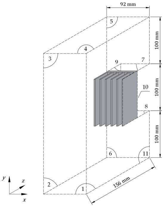
Figure 5. Computational domain with labeled outer boundaries (1–11).

5.2. Governing Equations

The described process is a 3D steady-state conjugate heat transfer problem involving conduction within the heat sink and natural convection in the surrounding air. A corresponding three-dimensional mathematical model has been defined, formulated under the following assumptions:

• The solid is homogeneous and isotropic, with constant thermophysical properties;
• Natural convection flow is steady, laminar, and driven solely by buoyancy, while density variations are accounted for using the incompressible ideal gas law formulation;
• All other fluid thermophysical properties are constant and evaluated at the film temperature;
• Viscous dissipation and effects of radiative heat transfer are neglected;
• Symmetry at mid-width is modeled as adiabatic and impermeable;
• Uniform temperature is assumed at the heat sink base;
• Ambient temperature far from the heat sink is constant.

Governing equations for each subdomain are given below. For the solid aluminum heat sink, the following energy equation is applied:

$${\displaystyle \frac{{\mathsf{\partial }}^{2}T}{\mathsf{\partial }{x}^2}}+{\displaystyle \frac{{\mathsf{\partial }}^{2}T}{\mathsf{\partial }{y}^2}}+{\displaystyle \frac{{\mathsf{\partial }}^{2}T}{\mathsf{\partial }{z}^2}}=0$$

(15)

For the fluid (air), continuity, three momentum (x, y, and z directions), and energy equations are applied:

$${\displaystyle \frac{\mathsf{\partial }\left[{\rho }_{\mathrm{a}}\left(T\right)w_x\right]}{\mathsf{\partial }x}}+{\displaystyle \frac{\mathsf{\partial }\left[{\rho }_{\mathrm{a}}\left(T\right)w_y\right]}{\mathsf{\partial }y}}+{\displaystyle \frac{\mathsf{\partial }\left[{\rho }_{\mathrm{a}}\left(T\right)w_z\right]}{\mathsf{\partial }z}}=0$$

(16)

$${\rho }_{\mathrm{a}}\left(T\right)\left(w_x{\displaystyle \frac{\mathsf{\partial }{w}_x}{\mathsf{\partial }x}}+w_y{\displaystyle \frac{\mathsf{\partial }{w}_x}{\mathsf{\partial }y}}+w_z{\displaystyle \frac{\mathsf{\partial }{w}_x}{\mathsf{\partial }z}}\right)=-{\displaystyle \frac{\mathsf{\partial }{p}^{*}}{\mathsf{\partial }x}}+{\mu }_{\mathrm{a}}\left({\displaystyle \frac{{\mathsf{\partial }}^2{w}_x}{\mathsf{\partial }{x}^2}}+{\displaystyle \frac{{\mathsf{\partial }}^2{w}_x}{\mathsf{\partial }{y}^2}}+{\displaystyle \frac{{\mathsf{\partial }}^2{w}_x}{\mathsf{\partial }{z}^2}}\right)$$

(17)

$$\begin{array}{l}{\rho }_{\mathrm{a}}\left(T\right)\left(w_x{\displaystyle \frac{\mathsf{\partial }{w}_y}{\mathsf{\partial }x}}+w_y{\displaystyle \frac{\mathsf{\partial }{w}_y}{\mathsf{\partial }y}}+w_z{\displaystyle \frac{\mathsf{\partial }{w}_y}{\mathsf{\partial }z}}\right)\\ =-{\displaystyle \frac{\mathsf{\partial }{p}^{*}}{\mathsf{\partial }y}}+{\mu }_{\mathrm{a}}\left({\displaystyle \frac{{\mathsf{\partial }}^2{w}_y}{\mathsf{\partial }{x}^2}}+{\displaystyle \frac{{\mathsf{\partial }}^2{w}_y}{\mathsf{\partial }{y}^2}}+{\displaystyle \frac{{\mathsf{\partial }}^2{w}_y}{\mathsf{\partial }{z}^2}}\right)+\left[{\rho }_{\mathrm{a}}\left(T\right)-{\rho }_{\mathrm{o}\mathrm{p}}\right]g_y\end{array}$$

(18)

$${\rho }_{\mathrm{a}}\left(T\right)\left(w_x{\displaystyle \frac{\mathsf{\partial }{w}_z}{\mathsf{\partial }x}}+w_y{\displaystyle \frac{\mathsf{\partial }{w}_z}{\mathsf{\partial }y}}+w_z{\displaystyle \frac{\mathsf{\partial }{w}_z}{\mathsf{\partial }z}}\right)=-{\displaystyle \frac{\mathsf{\partial }{p}^{*}}{\mathsf{\partial }z}}+{\mu }_{\mathrm{a}}\left({\displaystyle \frac{{\mathsf{\partial }}^2{w}_z}{\mathsf{\partial }{x}^2}}+{\displaystyle \frac{{\mathsf{\partial }}^2{w}_z}{\mathsf{\partial }{y}^2}}+{\displaystyle \frac{{\mathsf{\partial }}^2{w}_z}{\mathsf{\partial }{z}^2}}\right)$$

(19)

$${\rho }_{\mathrm{a}}\left(T\right)\left(w_x{\displaystyle \frac{\mathsf{\partial }T}{\mathsf{\partial }x}}+w_y{\displaystyle \frac{\mathsf{\partial }T}{\mathsf{\partial }y}}+w_z{\displaystyle \frac{\mathsf{\partial }T}{\mathsf{\partial }z}}\right)={\displaystyle \frac{k_{\mathrm{a}}}{c_{\mathrm{p},\mathrm{a}}}}\left({\displaystyle \frac{{\mathsf{\partial }}^{2}T}{\mathsf{\partial }{x}^2}}+{\displaystyle \frac{{\mathsf{\partial }}^{2}T}{\mathsf{\partial }{y}^2}}+{\displaystyle \frac{{\mathsf{\partial }}^{2}T}{\mathsf{\partial }{z}^2}}\right)$$

(20)

In the incompressible ideal gas law formulation, buoyancy-driven density variations are captured without solving the fully compressible Navier–Stokes equations. An operating pressure (p_op), most commonly the atmospheric pressure, is defined, and the local fluid density is computed via the ideal gas relation [25]:

$${\rho }_{\mathrm{a}}\left(T\right)={\displaystyle \frac{p_{\mathrm{o}\mathrm{p}}}{RT}}$$

(21)

In Equation (21), R [J/(kg·K)] is the specific gas constant. In Equations (17)–(19), p* [Pa] is the modified pressure after subtracting the hydrostatic part based on operating density. Operating density ρ_op [kg/m³] is the air density evaluated at the ambient temperature T_∞ [K] and the operating pressure p_op [Pa].

The temperature-dependent density field enters the continuity equation, ensuring mass conservation even with variable density. The buoyancy source term in the momentum equations produces an upward force wherever the fluid is warmer, i.e., lighter. Unlike the Boussinesq approximation, this density formulation is applicable for larger temperature differences, allowing the examination of a wider range of ambient and heat sink operating temperatures.

5.3. Boundary Conditions

Boundary conditions are defined at the domain outer boundaries (as denoted in Figure 5) and at the interface between the solid (heat sink) and fluid (air).

At the domain bottom boundary (1), a pressure inlet is imposed. It specifies zero-gauge pressure, with flow direction normal to the boundary, and constant temperature at the boundary, corresponding to ambient temperature:

$$p=p_{\mathrm{\infty }}$$

(22)

$${T=T}_{\mathrm{\infty }}$$

(23)

At the lateral (2), front (3), top (4), upper rear (5), and bottom rear (6) boundaries, pressure outlet conditions are applied. A zero-gauge pressure is specified, while in the event of backflow, the flow direction is aligned with that of the adjacent interior cells, and the backflow temperature is set equal to the ambient temperature:

$$p=p_{\mathrm{\infty }}$$

(24)

$${T=T}_{\mathrm{\infty }}$$

(25)

It should be noted that at pressure-specified boundaries, pressure is fixed, rather than velocity. Velocity at those boundaries is computed so that the continuity with outlet conditions and the internal flow field is satisfied.

Adiabatic wall and no-slip condition are defined at the upper (7) and lower (8) horizontal boundaries, as well as the rear vertical boundary (9) behind the heat sink:

$${\displaystyle \frac{\mathsf{\partial }T}{\mathsf{\partial }n}}=0$$

(26)

$$w_x=0$$

(27)

$$w_y=0$$

(28)

$$w_z=0$$

(29)

At the heat sink base (10), an isothermal boundary condition is imposed:

$$T=T_{\mathrm{b}}$$

(30)

A symmetry boundary condition is applied at the symmetry plane (11). It assumes that there is no flow or heat transfer normal to the symmetry plane and that all variables have zero gradient in the direction perpendicular to the plane. For both the solid and fluid, this implies the following:

$${\displaystyle \frac{\mathsf{\partial }T}{\mathsf{\partial }x}}=0$$

(31)

For the fluid subdomain, additional constraints are applied:

$$w_x=0$$

(32)

$${\displaystyle \frac{\mathsf{\partial }{w}_y}{\mathsf{\partial }x}}=0$$

(33)

$${\displaystyle \frac{\mathsf{\partial }{w}_z}{\mathsf{\partial }x}}=0$$

(34)

At the solid–fluid interface, the boundary layer heat transfer is defined, and a no-slip condition is enforced:

$$k_{\mathrm{A}\mathrm{l}}{\displaystyle \frac{\mathsf{\partial }T}{\mathsf{\partial }n}}=k_{\mathrm{a}}{\displaystyle \frac{\mathsf{\partial }T}{\mathsf{\partial }n}}$$

(35)

$$w_x=0$$

(36)

$$w_y=0$$

(37)

$$w_z=0$$

(38)

5.4. Numerical Procedure

The problem was solved numerically using the finite volume method [26,27], and the solution was obtained via the ANSYS Fluent 18.2 solver. The SIMPLE algorithm was employed for pressure–velocity coupling, ensuring that density remained a function of temperature only, rather than being influenced by local pressure fluctuations. For pressure discretization, the PRESTO! scheme was applied. Convective terms in both the momentum and energy equations were discretized using the second-order upwind scheme. To enhance numerical stability and promote convergence, an operating density corresponding to the ambient temperature was defined to stabilize the pressure field in the incompressible ideal gas formulation. In addition, under-relaxation factors of 0.3, 0.6, and 1 were applied to the pressure, momentum, and energy equations, respectively. Convergence is considered achieved when residuals dropped below 10⁻³ for the continuity equation and 10⁻⁶ for the momentum and energy equations.

To ensure mesh independence of the numerical results, a grid sensitivity analysis was conducted by comparing the specific heat flux at the heat sink surface for three mesh sizes: 525,900, 4,119,600, and 8,968,725 cells (Figure 6). The results exhibited minimal variation across all mesh configurations, with the smallest relative difference observed between the two finest meshes (with 4,119,600 and 8,968,725 cells), indicating that the solution is mesh-independent. Consequently, the mesh with 4,119,600 cells was selected for all subsequent simulations. The corresponding mesh configuration is shown in Figure 7. Different colors indicate the multi-block decomposition of the air subdomain; the blocks were laid out to match the fin passages and to align the surrounding enclosure with the heat sink geometry, enabling a structured hexagonal mesh.

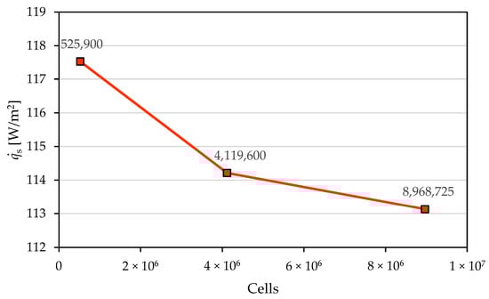
Figure 6. Comparison of considered mesh sizes.

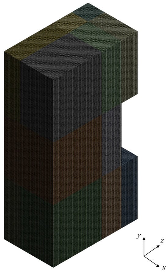
Figure 7. Selected mesh configuration.

6. Model Validation and Numerical Results

6.1. Model Validation

Results obtained numerically have been compared with experimental measurements. Accordingly, the operating conditions used in the numerical simulation were consistent with those in the performed experiment. The air inlet and backflow temperature were set to 29 °C (rounded from the experimentally obtained 29.02 °C), corresponding to the ambient conditions during testing. The heat sink base was maintained at a constant temperature of 50 °C, which represents the average value recorded during the steady-state interval of the experimental measurements. Atmospheric pressure (101,325 Pa) was specified at both the inlet and outlet to reflect the open environment of the test setup. The operating density was set to 1.17 kg/m³, consistent with the ambient temperature. The thermophysical properties of the air used were as listed in Table 2, whereas the thermal conductivity (k_Al) of aluminum was specified as 202.4 W/(m·K).

In order to validate the mathematical model and numerical procedure, a series of thermal parameters obtained numerically have been compared with those obtained from experimental measurements. Specific heat fluxes at the base (${\dot{q}}_{\mathrm{b}}$) and at the heat sink surface (${\dot{q}}_{\mathrm{s}}$), as well as average temperatures at the heat sink surface (T_s) and heat transfer coefficients (h), have also been compared, as shown in Table 5, along with respective deviations.

Table 5. Comparison of numerical predictions with experimental results and corresponding deviations.

Quantity	Numerical	Experimental	Deviation
${\dot{q}}_{\mathrm{b}}$ [W/m2]	770.28	749.37	2.79%
${\dot{q}}_{\mathrm{s}}$ [W/m2]	114.21	112.63	1.4%
Ts [°C]	49.83	49.63	0.06%
h [W/(m2·K)]	5.48	5.46	0.37%

As can be seen from Table 5, specific heat fluxes at the heat sink base (${\dot{q}}_{\mathrm{b}}$) and surface (${\dot{q}}_{\mathrm{s}}$) show deviations of 2.79% and 1.4%, respectively, indicating good agreement in predicted heat transfer rates. The average heat sink surface temperature (T_s) shows a good match, with a deviation of 0.06% relative to absolute temperature [K]. Finally, the heat transfer coefficient (h) shows a deviation of 0.37%. The observed deviations are within acceptable limits, thus validating the ability of the numerical model to accurately capture the physical phenomena of heat dissipation through the examined passive heat sink.

Additionally, temperature profiles along the characteristic fin height and length were compared between numerical and experimental results. Experimental profiles were taken at previously defined thermocouple positions (H_TC1 = 1 mm and H_TC2 = 15 mm at L = 50 mm; L_TC3 = 1 mm and L_TC4 = 99 mm at H = 29 mm). The comparison of numerical predictions with measured temperatures has been shown in Figure 8 and Figure 9.

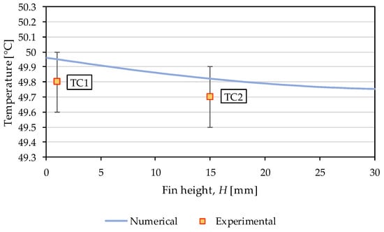
Figure 8. Comparison of numerically obtained temperature profiles along the representative fin height with experimentally measured temperatures at positions TC1 and TC2.

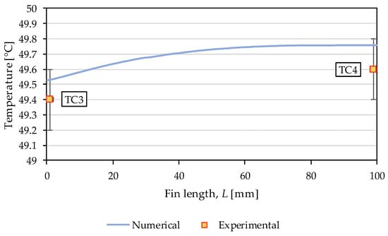
Figure 9. Comparison of numerically obtained temperature profiles along the representative fin length with experimentally measured temperatures at positions TC3 and TC4.

The comparison between the numerical and experimental temperature profiles along the fin height (Figure 8) and length (Figure 9) directions demonstrates good agreement, particularly when the accuracy of the thermocouples is considered. Along the fin height direction, a descending temperature gradient is observed as H increases, reflecting the conductive heat transfer from the heat sink base, where the temperature is highest. In contrast, along the fin length direction, an ascending temperature profile can be observed; the air near the bottom is coolest, leading to more intense heat transfer and lower surface temperatures in this region. As L increases, the surrounding air warms as it passes through the spacing between the fins, reducing the temperature gradient, resulting in slightly higher surface temperatures along the fin length.

These trends correspond to previously discussed experimental observations and further confirm the physical consistency between the experimental and numerical results.

6.2. Numerical Results

In order to further analyze natural convection behavior, temperature distributions and velocity vectors obtained using the validated numerical model have been shown in characteristic planes of the computational domain. The calculations were performed for the operating conditions of the conducted measurement: a base temperature of 50 °C and an ambient temperature of 29 °C. Figure 10 shows the temperature contours at the fins’ mid-height (H = 15 mm), while Figure 11 shows the temperature contours in the symmetry plane of the heat sink.

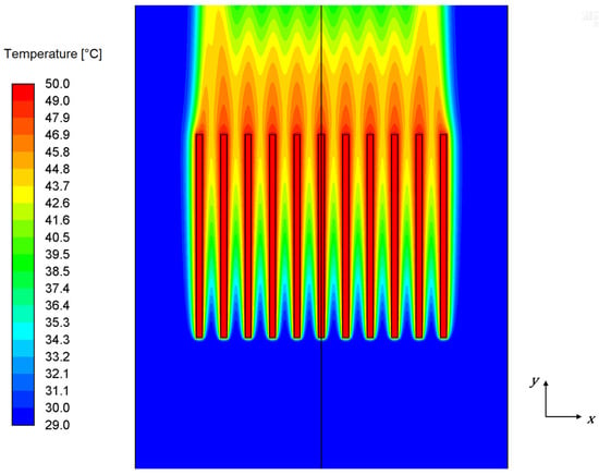
Figure 10. Temperature contours in the vertical plane at the fins’ mid-height (H = 15 mm) for a base temperature (T_b) of 50 °C and an ambient temperature (T_a) of 29 °C (T_b − T_a = 21 K).

Figure 11. Temperature contours in the symmetry plane for a base temperature (T_b) of 50 °C and an ambient temperature (T_a) of 29 °C (T_b − T_a = 21 K).

From Figure 10, it can be observed that heat dissipation through the heat sink is fairly uniform across all channels, i.e., within the spacings between adjacent fins. Boundary layers can be seen forming in between the surfaces of the fins, starting at the bottom as a result of buoyant upward motion of air particles, caused by heating from the fin surfaces, which creates localized plumes that rise between the fins. The temperature field indicates that air temperature is highest near the fin surfaces and gradually decreases toward the channel centerlines, which is consistent with typical thermal boundary layer development. Each channel between the fins acts like a miniature chimney, supporting the development of individual thermal plumes, which extend above the top of the heat sink, indicating an active heat removal via natural convection.

The symmetry plane temperature field (Figure 11) provides another view of the heat dissipation into the fluid subdomain. A characteristic plume of warm air is visible rising above the heat sink, consistent with buoyancy-driven flow, caused by the temperature difference between the heated fins and the ambient air. As the thermal plume ascends above the heat sink, it gradually becomes thinner. This is due to the entrainment of surrounding cooler air, which induces mixing and lateral thermal diffusion. Consequently, the temperature gradients subside, and the plume starts to diminish with height, becoming progressively narrower.

As seen in Figure 10 and Figure 11, the temperature distribution within the heat sink appears highly uniform. To examine this behavior more thoroughly, Figure 12 shows an isolated view of the heat sink, with the temperature scale adjusted from a global to a local range in order to more clearly capture subtle temperature variations.

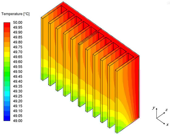
Figure 12. Local temperature contours on the heat sink surface for a base temperature (T_b) of 50 °C and an ambient temperature (T_a) of 29 °C (T_b − T_a = 21 K).

From Figure 12, it can be seen that the base of the heat sink, which is subjected to a constant temperature boundary condition, exhibits the highest temperature. Along the fin height, a gradual temperature decrease is observed, primarily due to heat conduction within the fin material and subsequent dissipation into the surrounding air via natural convection. The resulting temperature profile reflects the non-uniformity of heat transfer along the fin; the lower region remains cooler and is dominated by convective heat loss, driven by the larger temperature difference between the fin surface and the ambient air. As the air rises and becomes progressively warmer, the local temperature gradient decreases, thereby reducing convective heat transfer from the upper fin region. Additionally, the outer fins exhibit slightly lower temperatures compared to the inner ones, likely due to increased exposure to the surrounding cooler ambient air.

In order to examine the flow field, the distribution of velocity vectors in the fins’ mid-height plane (H = 15 mm) is presented in Figure 13.

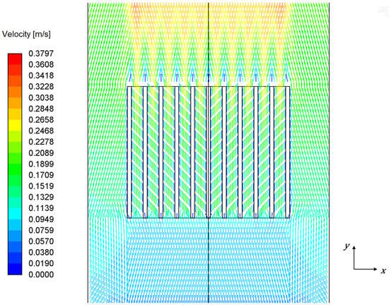
Figure 13. Velocity vectors in the vertical plane at the fins’ mid-height (H = 15 mm) for a base temperature (T_b) of 50 °C and an ambient temperature (T_a) of 29 °C (T_b − T_a = 21 K).

The velocity vector distribution, shown in Figure 13, provides a clear depiction of the buoyancy-driven airflow around the examined heat sink. At the bottom of the domain, where the pressure inlet is defined far from the heat sink, the velocity magnitude is minimal, indicating that the incoming ambient air is relatively inert. This is expected, as the air there is relatively cold and buoyancy forces are still weak. As air approaches the heat sink and is heated by the warm surfaces of the fins, its temperature increases, leading to a decrease in density. The density gradient gives rise to a buoyant force, which accelerates the fluid upward. As a result, an increase in velocity magnitude is observed in the spacing between the fins, as well as around the heat sink. Within the fin channels, the velocity vectors become more aligned in the vertical direction, indicating the formation of upward flow paths.

The velocity at the fin surfaces is zero due to the no-slip boundary condition applied at the solid–fluid interface. This enforces zero relative motion between the fluid and the solid walls and results in the formation of velocity boundary layers between the fins, as well as at the heat sink’s outer surfaces.

Above the heat sink, the flow accelerates further, forming the plumes. The highest velocities occur near the top of the enclosure, at the outlet region of the fin channels, where a pronounced upward jet of warm air is developed.

7. Analysis of the Influence of Operating Temperatures on Heat Sink Thermal Performance

7.1. Range Selection

To evaluate the influence of operating temperatures on the heat sink’s thermal performance, a parametric analysis was performed for different base and ambient temperatures.

Base temperatures of 50 °C, 65 °C and 80 °C were selected to represent typical operating conditions of low to moderately heated electronic components, such as processors under light load (corresponding to 50 °C), power transistors or voltage regulators in moderate thermal environments (operating at approximately 65 °C), and high-power devices or systems with limited cooling capacity (temperature of 80 °C).

Also, ambient temperatures of 19 °C, 24 °C, and 29 °C were considered to reflect representative environmental conditions ranging from air-conditioned indoor spaces (corresponding to 19 °C), to standard laboratory or office settings (temperatures of around 24 °C), to warmer industrial or passively ventilated environments (corresponding to 29 °C).

For the evaluation, three performance indicators were considered: total heat transfer rate ($\dot{Q}$), heat transfer coefficient (h), and overall thermal resistance (R).

In the numerical calculations, three different base temperatures were varied, along with three different ambient temperatures, covering all nine combinations of operating conditions. For clarity, the results are presented as functions of the temperature difference between the base and ambient air, and a list of investigated cases is provided in Table 6. Using base-to-ambient temperature difference as the independent variable collapses the data across cases and directly reflects the buoyancy driving potential under natural convection. Throughout the analysis, geometry parameters were held fixed, and properties were evaluated at the film temperature, so that observed trends can be attributed to operating temperatures alone.

Table 6. Operating conditions for the nine numerical cases.

Case	Tb [°C]	Ta [°C]	Tb − Ta [°C]
1	50	29	21
2	50	24	26
3	50	19	31
4	65	29	36
5	65	24	41
6	65	19	46
7	80	29	51
8	80	24	56
9	80	19	61

7.2. Influence on Heat Transfer Rate

In all calculations, heat transfer rate was obtained as the product of numerically obtained specific heat flux and the respective surface area. The influence of base-to-ambient temperature difference on heat transfer rate is shown in Figure 14.

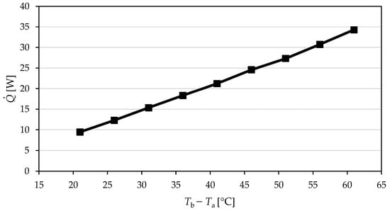
Figure 14. Influence of base-to-ambient temperature difference on heat transfer rate.

As seen from Figure 14, the heat transfer rate ($\dot{Q}$) increases almost linearly with the temperature difference between the heat sink base and ambient, ranging from 9.47 W at 21 °C to 34.28 W at 61 °C temperature difference. This behavior is expected since $\dot{Q}$ is directly proportional to the temperature gradient between the heat sink base and the ambient, the increase in which intensifies buoyancy-driven flow and thus increases heat dissipation from the heat sink surface.

7.3. Influence on Heat Transfer Coefficient

The heat transfer coefficient was obtained by dividing the numerically obtained specific heat flux on the heat sink surface by the temperature difference between the average heat sink surface temperature and the ambient temperature. The influence of base-to-ambient temperature difference on the heat transfer coefficient is provided in Figure 15.

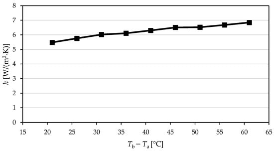
Figure 15. Influence of base-to-ambient temperature difference on the heat transfer coefficient.

It can be observed from Figure 15 that the heat transfer coefficient (h) increases from 5.48 to 6.84 W/(m²·K) as the surface-to-ambient temperature difference rises from 21 to 61 °C temperature difference. This rise reflects stronger buoyancy-driven natural convection at higher temperature differences, which enhances airflow around the fins and improves convective heat removal.

7.4. Influence on Overall Thermal Resistance

Overall thermal resistance R [K/W] is defined as the ratio of the base-to-ambient temperature difference and heat transfer rate:

$$R={\displaystyle \frac{T_{\mathrm{b}}-T_{\mathrm{a}}}{\dot{Q}}}$$

(39)

The influence of base-to-ambient temperature difference on the overall thermal resistance is presented in Figure 16.

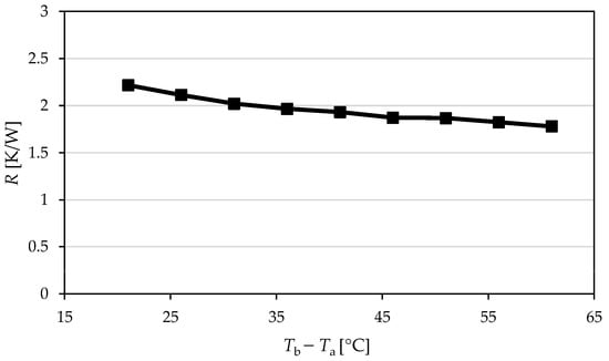
Figure 16. Influence of base-to-ambient temperature difference on the overall thermal resistance.

Figure 16 indicates that overall thermal resistance (R) decreases from 2.22 to 1.78 K/W as the temperature difference between the base and ambient increases. This is expected as the higher temperature difference strengthens buoyancy-driven convection in the channels between the fins, thus lowering the effective resistance.

7.5. Dimensionless Scaling

To further generalize the results and compare them with established natural convection models, the data were expressed in terms of the Nusselt number (Nu_s) and Rayleigh number (Ra_s). The Rayleigh number was calculated using the average heat sink surface temperature, with properties evaluated at respective film temperatures. Nusselt numbers were obtained in two ways: from the heat transfer coefficients obtained from the numerical results and by using the Bar-Cohen and Rohsenow correlation [11] given in Equation (12). The comparison, along with the best-fit power–-law correlation developed from the numerically obtained Nusselt values, is presented in Figure 17.

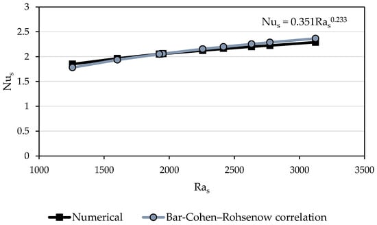
Figure 17. Spacing-based Nusselt number as a function of the Rayleigh number: comparison of numerical results with the Bar-Cohen–Rohsenow correlation [11].

As seen from Figure 17, numerically derived Nu_s values closely follow the correlation-predicted values across the investigated Rayleigh number range, spanning from approximately 1.25 × 10³ to 3.12 × 10³. The best-fit power-law correlation [28,29], obtained through the numerical data, yields the following:

$${\mathrm{N}\mathrm{u}}_{\mathrm{s}}=0.351{\mathrm{R}\mathrm{a}}_{\mathrm{s}}^{0.233}$$

(40)

The Bar-Cohen and Rohsenow framework for laminar natural convection in vertical parallel plate channels predicts a Rayleigh number exponent of 0.25. The present fit yields 0.233, which is mostly consistent with this trend. The fitted constant of 0.351 also matches the conventional vertical plate Nu–Ra coefficient range (0.33–0.36) for s/L ratios near 0.1. The close agreement with the classical vertical parallel plate correlation is expected for the present regime and geometry. The cases considered lie in the laminar natural convection range (with spacing-based Rayleigh numbers Ra_s of approximately 1.2 × 10³ to 3.6 × 10³), with quiescent air, vertical orientation, film temperature properties, and spacing-based nondimensionalization consistent with the correlation’s assumptions. Accordingly, the correlation applies to vertical, quiescent air operation with Pr ≈ 0.706, s/L = 0.09, and the stated Ra_s range. Extrapolation beyond these conditions (e.g., markedly different s/L, inclination, strong radiation, or higher Ra_s) should be treated with caution and validated against experiment or 3D simulation.

The small deviation from an exact exponent of 0.25 can be attributed to the limited Ra span, property evaluation, and modeling assumptions. Overall, for the conditions defined above, the scaling and numerical results are consistent with classical laminar natural convection theory and published results for vertical plate fin arrays.

8. Conclusions

In this paper, the thermal performance of a passive aluminum vertical heat sink with plate fins was comprehensively examined through both experimental measurement and numerical simulations. A custom-built experimental setup consisting of a water-filled vessel with the heat sink mounted on the side enabled measurement of water bulk temperature and fin surface temperatures during steady-state operation. From these measurements, the heat transfer rate and heat transfer coefficient were determined, with the latter showing good agreement with established correlations following comparison. A corresponding mathematical model and numerical procedure were developed and validated against experimental measurements and literature correlations, with the numerical results aligning well with both.

A parametric analysis was conducted, assessing the influence of operating base (50, 65, and 80 °C) and ambient temperatures (19, 24, and 29 °C), with temperature differences ranging from 21 to 61 °C. This analysis quantified key thermal performance indicators: heat transfer rate, heat transfer coefficient, and overall thermal resistance. The results showed a substantial increase in heat transfer rate with rising temperature difference, while the increase in heat transfer coefficient and the decrease in thermal resistance were milder in comparison. Additionally, a correlation between the Nusselt and Rayleigh numbers was established, providing the means for predicting the thermal behavior of similar natural convection-governed heat sinks.

Overall, the validated experimental–numerical framework provides a solid foundation for further studies on similar heat sink geometries and operating conditions. The framework is readily extendable to novel fin topologies (e.g., interrupted, chevroned, branched, or porous inserts), providing a screening tool for future design exploration under natural convection, and it can be directly extended to PCM-assisted heat sinks by incorporating an enthalpy-based PCM model. Beyond geometry, future work will consider transient operation and combined convective–radiative heat transfer to further enhance the thermal management of electronic systems.

References

- Ghadim, H.B.; Davodi, M.M.; Rezaei, F.; Jafari, A.; Eslami, M. Review of thermal management of electronics and phase change materials. Renew. Sustain. Energy Rev. 2025, 208, 115039. [Google Scholar] [CrossRef]
- Öztürk, E.; Tari, I. Forced air cooling of CPUs with heat sinks: A numerical study. IEEE Trans. Compon. Packag. Technol. 2008, 31, 650–660. [Google Scholar] [CrossRef]
- Kazem, H.A.; Al-Waeli, A.H.A.; Chaichan, M.T.; Sopian, K.; Al-Amery, A.; Wan Nor Roslam, W.I. Enhancement of photovoltaic module performance using passive cooling (Fins): A comprehensive review. Case Stud. Therm. Eng. 2023, 49, 103316. [Google Scholar] [CrossRef]
- Ismail, M. Experimental and numerical analysis of heat sink using various patterns of cylindrical pin-fins. Int. J. Thermofluids 2024, 23, 100737. [Google Scholar] [CrossRef]
- Lorenzini, M.; Fabbri, G.; Salvigni, S. Performance evaluation of a wavy-fin heat sink for power electronics. Appl. Therm. Eng. 2007, 27, 969–975. [Google Scholar] [CrossRef]
- El Ghandouri, I.; El Maakoul, A.; Saadeddine, S.; Meziane, M. Design and numerical investigations of natural convection heat transfer of a new rippling fin shape. Appl. Therm. Eng. 2020, 178, 115670. [Google Scholar] [CrossRef]
- Lyman, A.C.; Stephan, R.A.; Thole, K.A.; Zhang, L.W.; Memory, S.B. Scaling of heat transfer coefficients along louvered fins. Exp. Therm. Fluid Sci. 2002, 26, 547–563. [Google Scholar] [CrossRef]
- Shan, X.; Liu, B.; Zhu, Z.; Bennacer, R.; Wang, R.; Theodorakis, P.E. Analysis of the heat transfer in electronic radiator filled with metal foam. Energies 2023, 16, 4224. [Google Scholar] [CrossRef]
- Tari, I.; Mehrtash, M. Natural convection heat transfer from horizontal and slightly inclined plate-fin heat sinks. Appl. Therm. Eng. 2013, 61, 728–736. [Google Scholar] [CrossRef]
- Elenbaas, W. The dissipation of heat by free convection from vertical and horizontal cylinders. J. Appl. Phys. 1948, 19, 1148–1154. [Google Scholar] [CrossRef]
- Bar-Cohen, A.; Rohsenow, W.M. Thermally optimum spacing of vertical, natural convection-cooled, parallel plates. J. Heat Transf. 1984, 106, 116–123. [Google Scholar] [CrossRef]
- Ahmadi, M.; Mostafavi, G.; Bahrami, M. Natural convection from rectangular interrupted fins. Int. J. Therm. Sci. 2014, 82, 62–71. [Google Scholar] [CrossRef]
- Quintino, A.; Cianfrini, M.; Petracci, I.; Spena, V.A.; Corcione, M. Dimensionless correlations for natural convection heat transfer from a pair of vertical staggered plates suspended in free air. Appl. Sci. 2021, 11, 6511. [Google Scholar] [CrossRef]
- Shen, Q.; Sun, D.; Xu, Y.; Jin, T.; Zhao, X. Orientation effects on natural convection heat dissipation of rectangular fin heat sinks mounted on LEDs. Int. J. Heat Mass Transf. 2014, 75, 462–469. [Google Scholar] [CrossRef]
- Fuse, H.; Oe, S.; Haga, T. Effects of fin height, base thickness, blackening, emissivity and thermal conductivity on heat dissipation of die-cast aluminum alloy heat sink. Metals 2025, 15, 696. [Google Scholar] [CrossRef]
- Dewilde, L.; Ali, S.M.; Nimmagadda, R.; Persoons, T. On the numerical investigation of natural-convection heat sinks across a wide range of flow and operating conditions. Fluids 2024, 9, 252. [Google Scholar] [CrossRef]
- Lee, M.; Kim, H.J.; Kim, D.-K. Nusselt number correlation for natural convection from vertical cylinders with triangular fins. Appl. Therm. Eng. 2016, 93, 1238–1247. [Google Scholar] [CrossRef]
- Rao, A.K.; Somkuwar, V. Heat transfer of a tapered fin heat sink under natural convection. Mater. Today Proc. 2021, 46, 7886–7891. [Google Scholar] [CrossRef]
- Joo, Y.; Kim, S.J. Comparison of thermal performance between plate-fin and pin-fin heat sinks in natural convection. Int. J. Heat Mass Transf. 2015, 83, 345–356. [Google Scholar] [CrossRef]
- Huang, X.; Shi, C.; Zhou, J.; Zhang, L.; Xu, Z. Performance analysis and design optimization of heat pipe sink with a variable height fin array under natural convection. Appl. Therm. Eng. 2019, 160, 113939. [Google Scholar] [CrossRef]
- Fadiga, T. Investigation of Heat Transfer Through a Heat Sink. Master’s Thesis, Faculty of Engineering, University of Rijeka, Rijeka, Croatia, 2025. (In Croatian). [Google Scholar]
- Moffat, R.J. Describing the uncertainties in experimental results. Exp. Therm. Fluid Sci. 1988, 1, 3–17. [Google Scholar] [CrossRef]
- Sobhan, C.B.; Venkateshan, S.P.; Seetharamu, K.N. Experimental studies on steady free convection heat transfer from fins and fin arrays. Wärme-Und Stoffübertragung 1990, 25, 345–352. [Google Scholar] [CrossRef]
- Churchill, S.W.; Chu, H.H.S. Correlating equations for laminar and turbulent free convection from a vertical plate. Int. J. Heat Mass Transf. 1975, 18, 1323–1329. [Google Scholar] [CrossRef]
- ANSYS, Inc. In Ansys Fluent Theory Guide (Release 2024 R1); Section: Density—Incompressible Ideal Gas; ANSYS, Inc.: Canonsburg, PA, USA, 2024.
- Patankar, S.V. Numerical Heat Transfer and Fluid Flow; (1980/2018); CRC Press: Boca Raton, FL, USA, 2018. [Google Scholar] [CrossRef]
- Versteeg, H.K.; Malalasekera, W. An Introduction to Computational Fluid Dynamics: The Finite Volume Method, 2nd ed.; Pearson: London, UK, 2007. [Google Scholar]
- Heindel, T.J.; Ramadhyani, S.; Incropera, F.P. Laminar natural convection in a discretely heated cavity: I—Assessment of three-dimensional effects. J. Heat Transf. 1995, 117, 902–909. [Google Scholar] [CrossRef]
- Heindel, T.J.; Incropera, F.P.; Ramadhyani, S. Laminar natural convection in a discretely heated cavity: II—Comparisons of experimental and theoretical results. J. Heat Transf. 1995, 117, 910–917. [Google Scholar] [CrossRef]
Disclaimer/Publisher’s Note: The statements, opinions and data contained in all publications are solely those of the individual author(s) and contributor(s) and not of MDPI and/or the editor(s). MDPI and/or the editor(s) disclaim responsibility for any injury to people or property resulting from any ideas, methods, instructions or products referred to in the content. |
© 2025 by the authors. Licensee MDPI, Basel, Switzerland. This article is an open access article distributed under the terms and conditions of the Creative Commons Attribution (CC BY) license (https://creativecommons.org/licenses/by/4.0/).