Article

Simulation of Single Vapor Bubble Condensation with Sharp Interface Mass Transfer Model

Institute of Fluid Mechanics (ISTM), Karlsruhe Institute of Technology (KIT), 76131 Karlsruhe, Germany
*
Author to whom correspondence should be addressed.
Thermo 2022, 2(3), 149-159; https://doi.org/10.3390/thermo2030012
Submission received: 23 May 2022 / Revised: 27 June 2022 / Accepted: 28 June 2022 / Published: 30 June 2022

Abstract

:
Pure numerical simulation of phase-change phenomena such as boiling and condensation is challenging, as there is no universal model to calculate the transferred mass in all configurations. Among the existing models, the sharp interface model (Fourier model) seems to be a promising solution. In this study, we investigate the limitation of this model via a comparison of the numerical results with the analytical solution and experimental data. Our study confirms the great importance of the initial thermal boundary layer prescription for a simulation of single bubble condensation. Additionally, we derive a semi-analytical correlation based on energy conservation to estimate the condensing bubble lifetime. This correlation declares that the initial diameter, subcooled temperature, and vapor thermophysical properties determine how long a bubble lasts. The simulations are carried out within the OpenFOAM framework using the VoF method to capture the interface between phases. Our investigation demonstrates that calculation of the curvature of interface with the Contour-Based Reconstruction (CBR) method can suppress the parasitic current up to one order.

1. Introduction

Bubble condensation is an essential phenomenon for the description of heat and mass transfer in subcooled boiling. It is encountered in many industrial applications, such as microreactors or microchannels, where the bubble dynamics influence the cooling capacity and introduce instabilities to a robust operating condition [1,2]. The size and the shape of vapor bubbles change continuously during the condensation process, and this phenomenon significantly affects the flow structure. In order to better understand subcooled boiling, it is vital to obtain extensive knowledge of the condensing bubbles’ behavior.
Even though many experiments have been conducted on this topic [3], they are still limited to specific liquid properties or specific operating conditions. Moreover, experimental studies based on visualization with high-speed videography or PIV capture the bubble shape evolution but rarely provide detailed information on flow quantities such as temperature and pressure field. In the past decades, the numerical solvers evolved to provide more detailed information on the interface evolving phenomena such as vapor condensation. In reality, the interface between two phases is not sharp; it has a finite width, where the thermophysical properties change smoothly [4,5]. The interface thickness varies with temperature [6] or pressure [7] but remains in the range of a few nanometers [8]. It is not feasible to capture this thin transition region with conventional grid-based methods. Particle-based methods such as molecular dynamic (MD) can be employed to understand the process of formation of an equilibrium liquid-gas interface at the microscopic level [9,10]. The detailed physical insights obtained from MD simulations during phase-change [11,12,13] are utilized to apply appropriate boundary conditions or initial conditions around the liquid-gas interface in meso-scale or macro-scale simulations. Correspondingly, the interfacial region fits into one computational cell in these simulations, so the interface is assumed to be sharp. There are two general approaches for macro-scale simulations: two-fluid (Euler-Euler) methods and one-fluid methods [14]. The Euler-Euler method divides the gas-liquid into the continuous gas phase and the continuous liquid phase, and for each phase, the mass, momentum, and energy conservation equations are solved separately. It is the most practical method to simulate a two-phase system on a large macroscopic scale, as it requires lower grid resolution and is computationally less expensive compared to one-fluid methods [15]. However, this method is not in closed form and needs additional interaction terms depending on the two-phase flow regimes present. With different relationships under different flow regimes, it might be difficult to obtain an accurate solution for realistic scenarios [14,15]. The one-fluid method is sometimes termed direct numerical simulation for a two-phase system, as no assumptions or models for the interface shape are employed [16,17]. The one-fluid methods are classified into: sharp interface, such as Level-Set (LS) [18] and Volume-of-Fluid (VoF) [19,20], and diffuse interface, such as phase-field [21]. The one-fluid methods are applied for the simulation of a single vapor bubble condensation widely, but the main challenge in such numerical simulations is a reliable and physical computation of the mass transfer through the interface. Unfortunately, the mass transfer models are often based on semi-empirical correlations and hence are rarely generally applicable.
The Lee model [22] is one of the most popular mass transfer models. It assumes that mass is transferred at a constant pressure in a phase change flow system, and the model is derived for a quasi-thermo-equilibrium state:
m ˙ = r c α l ρ l T T s a t T s a t , for condensation T < T s a t .
where α (-) is the phase volume fraction and ρ (kg/m3) is density. The subscripts l and g represent the liquid and vapor phases, respectively. The volumetric mass flux m ˙ (kg/m3s) depends highly on the relaxation parameter r c (s−1). A wide range between 0.1 and 10 6 s−1 is proposed and successfully used for r c in previous studies [23]. Li et al. [24] derived a correlation for the relaxation parameter and showed the dependence of r c on the temperature, physical properties, and phase volume fraction of the grid element.
Another widespread model was derived by Tanasawa [25] based on the Schrage phase change model [26]. Schrage computed the interfacial mass flux m ˙ (kg/m2s) using Hertz–Knudsen equation assuming a jump in the temperature and pressure across the interface T s a t p l = T l T s a t p g = T g :
m ˙ = 2 2 γ c M 2 π R γ c p g T g γ e p l T l ,
where R = 8.314 (J/mol K) is the universal gas constant, M (kg/mol) is the molar mass, and γ is the fraction of molecules transferred from one phase to the other. The subscripts c and e refer to condensation and evaporation, respectively. γ c  = 1 means all vapor molecules hitting the interface are converted to liquid. In the numerical simulation, usually, γ c = γ e is considered. Tanasawa assumed the interface is at saturation temperature and the mass flux varies linearly with temperature difference and the bulk temperature. He simplified Equation (2) to:
m ˙ = 2 γ 2 γ M 2 π R ρ g h l g T T s a t T s a t 3 / 2 , m ˙ = m ˙ A V ,
where h l g (J/kg) is the latent heat, V (m3) is the cell volume, and A (m2) is the interfacial area in each cell obtained from the interface reconstruction technique (see Section 2.2). In Equations (2) and  (3), the computed mass flux depends on the empirical parameter γ . The γ = 0.1 1 is suggested for dynamically renewing water surfaces such as jets and moving films and γ < 0.1 for stagnant surfaces [27]. Samkhaniani and Ansari [28] report that the bubble lifetime is highly sensitive to the choice of γ in vapor condensation simulations and suggest that an appropriate value must be selected for simulations in comparison with experiments.
A wider list of available mass transfer models is given in ref. [29]. Almost all available models suffer from a dependence on tuning parameters. In the present study, the sharp interface model is employed where the mass transfer is calculated based on a heat flux balance using the Fourier equation:
m ˙ = q h l g = k l T k g T h l g , m ˙ = m ˙ A V ,
where k (w/m K) is the thermal conductivity. The main objective of the present study is to investigate the sharp interface model predictive capability for vapor bubble condensation in comparison with experiments and the Tanasawa model. Moreover, the model limitations are reported.

2. Methodology and Validation

Both liquid and vapor are treated as an incompressible and immiscible Newtonian fluid mixture. The interface between the two phases is resolved using the volume-of-fluid method (VoF) in OpenFOAM solver interFoam, which has been extended with the CBR method [30]. The reconstruction part is essential for an accurate mass flux rate and interface curvature calculation. This improves the surface tension estimation and reduces the parasitic current [31] by up to one order of magnitude (see Section 2.2). The two-phase Navier–Stokes equation in a single-fluid formulation is solved within the PIMPLE (merged PISO-SIMPLE) algorithm loop. The solver is extensively applied for simulations of boiling [30,32,33] and recently ported to OpenFOAM-6.
The following governing equations are utilized:
  • Mass conservation
    ρ t + · ρ u = m ˙ ,
  • Momentum conservation
    ρ u t + · ρ uu · μ u + u T = p + ρ g + κ σ α l ,
  • Energy conservation
    ρ c p T t + · ρ c p T u · k T = m ˙ h l g ,
  • Phase-fraction transport equation
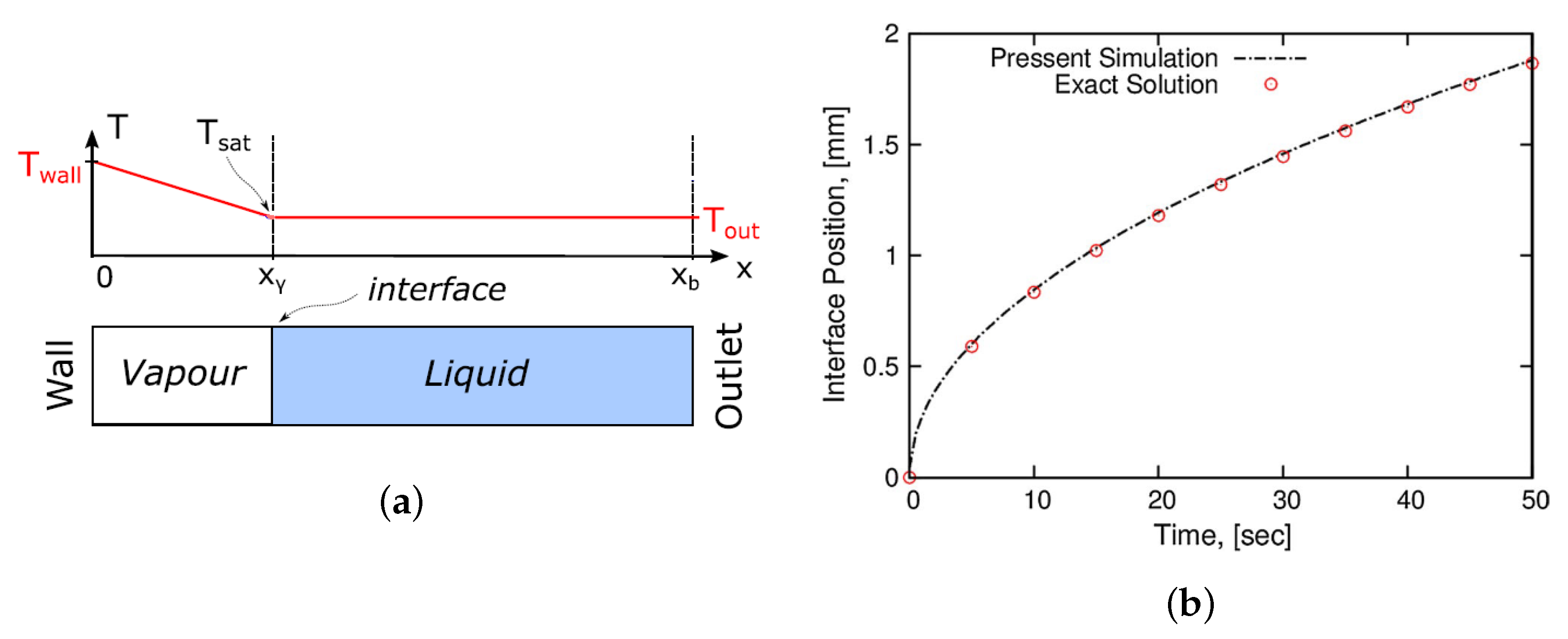
    α l t + · α l u = m ˙ α l ρ .
Here α l = V l V c e l l is the liquid volume fraction, while the physical properties such as density, heat capacity, thermal conductivity, and viscosity θ ρ , c p , k , μ are estimated with linear interpolation θ = θ l α l + θ g ( 1 α l ) in the interfacial region. The last term in the momentum equation, Equation (6), represents the surface tension force between two phases using a continuous surface force (CSF) model [34], where the interface curvature κ is obtained from the CBR method. In the present study, the volumetric mass transfer m ˙ due to condensation is calculated with the Fourier model from Equation (4).

2.1. Stefan Problem

The classical one-dimensional Stefan problem is applied to validate the phase change models. The problem setup has been extensively used for the validation of mass transfer models [20,35,36]. The schematic of the problem and the comparison with the analytical solution are shown in Figure 1. The exact solution for interface position x i (m) is calculated as:
x i ( t ) = 2 η d g t ,
where t (s) is time and d g = k / ρ c p (m2/s) is the vapor thermal diffusivity, and η is obtained from:
η exp ( η ) erf ( η ) = c p T w a l l T s a t π h l g .
The details of the test-case setup, including boundary conditions and the thermophysical properties, correspond to the ones reported in the previous study by Samkhaniani and Ansari [23]. The comparison with the analytical solution confirms that the sharp interface method is capable of accurately predicting the analytical solution.

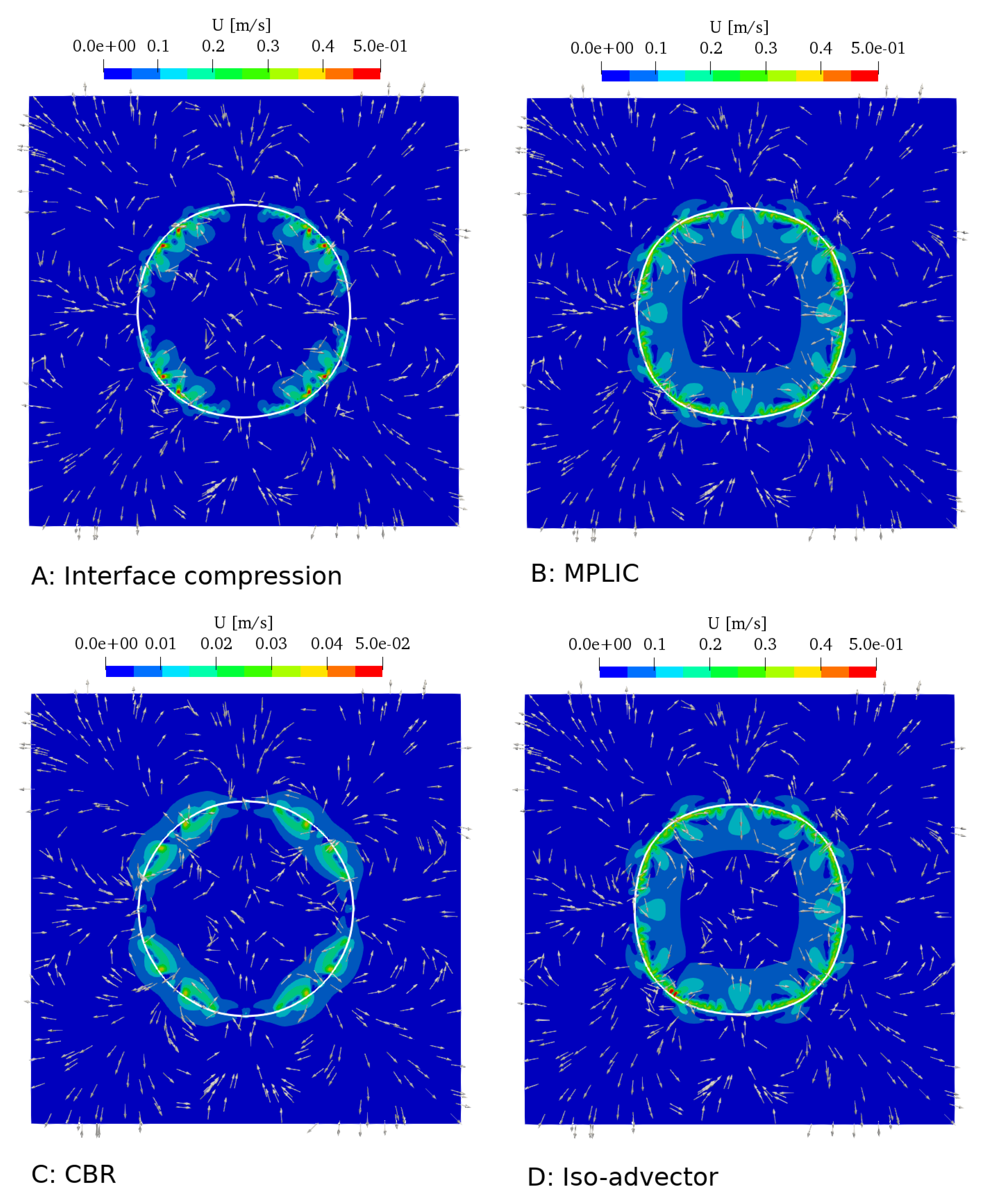
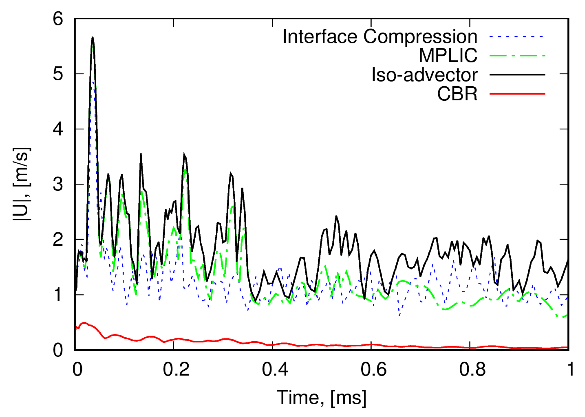
2.2. Parasitic Current

The spurious (parasitic) current is described as nonphysical velocity created near the interface region as a result of the numerical imbalance between surface tension force and pressure gradient force. This current is intensified where the surface tension becomes dominant.
The strength of the parasitic current is often measured with the maximal magnitude of velocity u for a single bubble placed in a stagnant liquid in zero gravity in the absence of phase change. The current may distort the interface [31] or impair the mass transfer estimation during phase change [28], rendering nonphysical results. Thus, it is crucial to improve surface tension modeling to avoid the parasitic current.
The conventional OpenFOAM VoF solver for simulations of the incompressible immiscible two-phase systems is interFoam [37]. It is an algebraic VoF method that does not reconstruct interface geometrically. The solver employs the Multidimensional Universal Limiter with Explicit Solution (MULES) technique with an additional interface compression term · ( α l ( 1 α l ) u c ) to Equation (8) to keep the interface sharp within 2 or 3 computational cells [38]. The compression velocity u c is calculated in the normal direction to the interface. This extra term acts only in the interfacial region to suppress numerical smearing in the α -field. Recently, the geometric VoF methods, such as the iso-advector method [39,40], and some variants of Piecewise the Linear Interface Calculation (PLIC) method [41], like Multicut Piecewise-Linear Interface Calculation (MPLIC) [42], have been implemented in the OpenFOAM framework. Those methods geometrically reconstruct the interface on polyhedral mesh, which improves the interface sharpness and provides a more accurate curvature estimation. In the present study, the CBR method [30] reconstructs the interface at iso-surface α l = 0.5 , which is then used only for the calculation of curvature κ , not for the phase flux calculation correction.
In order to investigate the performance of various VoF methods regarding spurious current, a 2-dimensional gas bubble with the diameter D 0 = 2 mm is placed in the centre of the computational domain with the size of 2 D 0 × 2 D 0 and filled with a quiescent liquid. Uniform hexahedral cells ( Δ x = D 0 / 100 ) are utilized for domain discretization. The liquid and gas physical properties are ρ l = 1000 kg/m3, ν l = μ l / ρ l = 10 6 m2/s, ρ g = 1 kg/m3, ν g = μ g / ρ g = 10 6 m2/s, σ = 0.1 N/m. The pressure value at the boundaries is considered as uniformly constant and equal to zero and the Neumann boundary condition is assigned for velocity.
The spurious current contour is displayed in Figure 2 for four considered VoF methods. In geometric VoF methods (case B and D), the parasitic current influences a thicker region around the interface and the bubble deviates from its initial spherical shape. As the density of the gas is much smaller than the liquid, the imbalance force accelerates the gas, and a higher velocity is observed on the gas side. The magnitude of the parasitic current in the CBR method is at least one order of magnitude smaller compared to the other methods provided by the standard interFoam implementation, as shown in Figure 3, where the time history of the maximal magnitude of the parasitic current is plotted.

3. Results and Discussion

In this section, a single vapor bubble of condensation is simulated with the Fourier model. The bubble lifetime is compared with experiments and previous numerical simulation based on the Tanasawa mass transfer model. In conclusion, a semi-analytical correlation for the bubble’s life is proposed.

3.1. Problem Definition
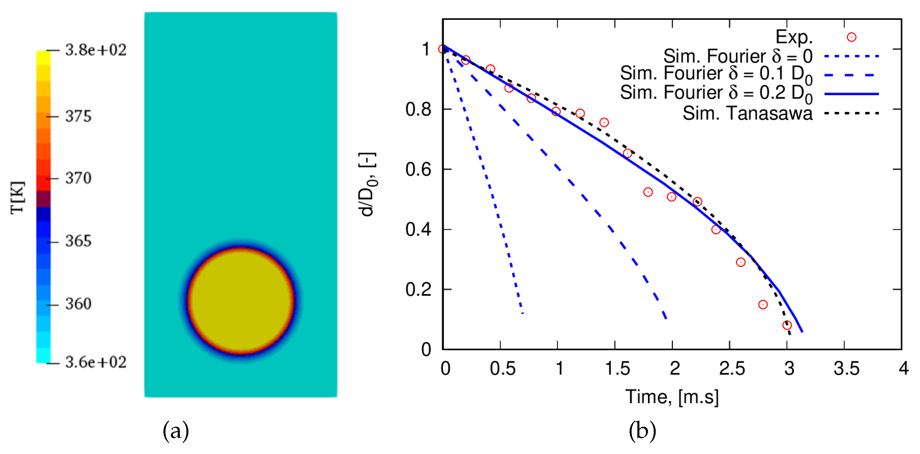
The rising of a single vapor bubble is simulated similar to [28,43]. The bubble is introduced at the saturated temperature T s a t = 380.2 K at P s a t = 0.13 MPa and is surrounded by quiescent water at T i n f = 355.2 K corresponding to a 25 K subcooling temperature. The thermophysical properties for vapor are ρ = 0.754 kg/m3, ν = 1.66 × 10 5 m2/s, k = 0.0259 W/m K, c p = 2110.7 J/kg K, and for liquid water ρ = 953.1 kg/m3, ν = 2.75 × 10 7 m2/s, k = 0.68 W/m K, c p = 4224.4 J/kg K. The surface tension σ = 0.057 N/m, latent heat h l g = 2237 kJ/kg, and gravity g = 9.81 m/s2 are used [43,44]. The computational domain size is 2 D 0 × 4 D 0 and filled with 100 × 200 uniform hexahedral cells, which corresponds to 50 cells per diameter. The initial diameter of the vapor bubble is D 0 = 1.008 mm, located at the middle line with distance D 0 from the bottom patch. There is a thin thermal region around the interface where the temperature smoothly changes from a saturated temperature inside the bubble to the subcooled temperature of the surrounding liquid. The temperature profile inside this region is initialized with [45]:
T r = a r 2 b r + c , a = T s a t T i n f δ 2 , b = 2 a D 0 2 + δ , c = T i n f + a D 0 2 + δ 2 ,
where r (m) is the distance to the bubble centre and δ (m) is the thickness of the thermal region. At the boundaries, the uniform constant dynamic pressure ( p d = 0 Pa) and temperature ( T = T i n f ) are introduced, while the velocity gradient and volume fraction gradient are set to be zero.

3.2. Validation

The bubble shape sequence is compared with an experiment from [43] and a previous numerical simulation [28] in Figure 4, and the result shows qualitatively good agreement. The vapor bubble condenses while moving upward and accelerates as it becomes smaller.
For quantitative comparison, the bubble’s lifetime is plotted against experimental data in Figure 5. Simulation of bubble evolution with the Fourier model for δ 0.2 D 0 coincides well with the experimental data [43] and previous numerical simulation [28].

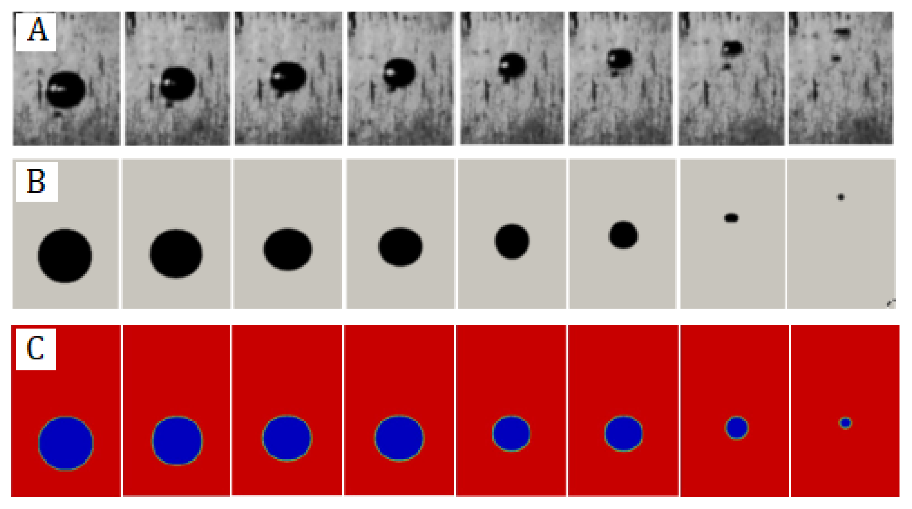
3.3. Thermal Boundary Layer

The bubble’s initial temperature profile is shown in Figure 5a. The bubble lifetime is influenced by this thin thermal region around the interface, as given in Figure 5b. It shows that when no thermal boundary region is defined, the bubble collapses too fast. In contrast, a thicker thermal boundary layer around the interface slows down the process and prolongs the bubble’s lifetime. The results indicate the importance of the sub-millimeter region around the interface for the bubble condensate rate. It is the most influencing parameter in the considered simulation with the Fourier model. Unfortunately, experimental studies often do not provide any information about this thermal boundary layer. A comparison with experimental data without the knowledge of the exact temperature field in the vicinity of the interface in the initial state of a simulation is a trial-and-error process since an accurate prescription of the temperature distribution in this tiny region is rather difficult.
In the present numerical simulation, a pure substance fluid is considered. Obviously, in real-world scenarios, there will practically always be some impurities involved, e.g., nitrogen, oxygen and carbon dioxide solved in the water. In such mixtures, a light boiling component (non-condensable gas) will usually accumulate at the interface [46,47]. This accumulation may act as a barrier to mass transfer [10,11,48]. It has been shown that even very small mole fractions of a non-condensable gas solved in the liquid might change the overall dynamics of the system and reduce the mass transfer rate significantly [49,50]. Thus, additionally to the thermal boundary layer, the non-condensable gases can hinder the mass transfer rate. As an alternative option, Tanasawa mass transfer model might be recommended since the mass coefficient λ can indirectly account for the missing thermal boundary layer information and/or non-condensable gas effect. The effect of these gases might be considered in future work, but it remains out of the scope of the present study.

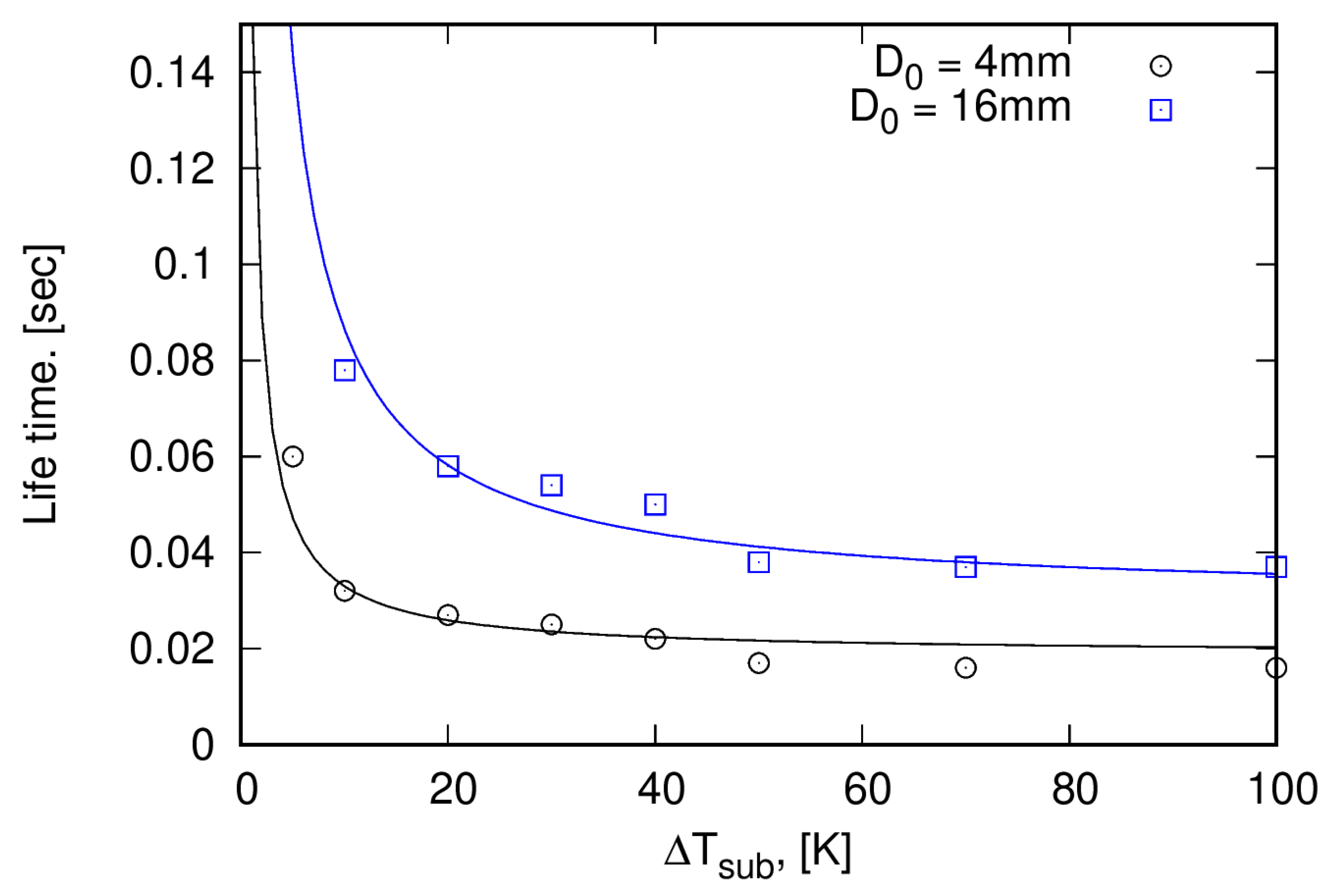
3.4. Bubble Lifetime

The lifetimes of bubbles at various subcooled temperatures Δ T s u b = [ 5 100 ] K obtained from numerical simulations are plotted in Figure 6. The trend is similar for both diameters D 0 = 4 , 16 mm. The mass transfer rate is driven by the temperature difference between the vapor bubble at saturation temperature and the bulk liquid in the subcooled temperature. Therefore, at low subcooled temperatures, the bubble is maintained for a longer period of time. However, there is a limitation to the total heat capacity that can be transferred in a definite portion of time using the conduction and convection modes. Thus, at higher subcooled temperatures, the bubble’s lifetime becomes almost constant. The overall trend is also observed in Sideman et al.’s experiments [51]. A simplified correlation is derived for the bubble’s lifetime based on energy conservation around the bubble in Equation (12):
t b = ρ c p T s a t + h l g D 0 2 f 1 Δ T s u b + f 2 ,
where f 1 and f 2 are fitting coefficients obtained via comparing with numerical simulations. f 1 represents the effective heat transfer coefficient h e f f at the beginning of bubble condensation. Assume f 2 = f 3 D 0 3 (s), then the coefficients are f 1 = 32 , 440 W/m2K and f 3 = 0.12 s/m1/3. This correlation reveals how bubble lifetime varies with bubble diameter, subcooled temperature, and latent heat. The details of the derivation can be found in Appendix A.

4. Conclusions

In the present paper, single vapor bubble condensation is modeled with the sharp interface Fourier mass transfer model. The model is proven to be highly accurate via comparison with the analytical solution for the case of the Stefan problem. It does not require any fitting parameters. However, the numerical model is sensitive to the initial thermal field, which is usually unknown for a particular configuration case. Therefore, in future work, we aspire to identify a correlation for estimating the thermal boundary region’s thickness around the bubble based on further experimental or analytical studies.
Additionally, a correlation for the bubble’s lifetime is derived based on the energy balance. The correlation shows good agreement with numerical simulation and relates the dependence of the condensing bubble’s lifetime to the initial diameter, subcooled temperature, and physical properties of the considered fluids.

Author Contributions

N.S.: Conceptualization, methodology, software, validation, formal analysis, investigation, writing—original draft preparation, visualization. A.S.: writing—review and editing, project administration, funding acquisition. All authors have read and agreed to the published version of the manuscript.

Funding

We gratefully acknowledge the financial support by the German Research Foundation (DFG) through the Research Unit 2383 ProMiSe under Grant No. STR 1585/2-1.

Institutional Review Board Statement

Not applicable.

Informed Consent Statement

Not applicable.

Data Availability Statement

Not applicable.

Acknowledgments

We would like to thank Martin Wörner and the reviewers for their detailed comments and suggestions, which improved the manuscript.

Conflicts of Interest

The authors declare no conflict of interest.

Appendix A. Bubble Lifetime Estimation

During the condensation, heat transfers from a condensing vapor bubble to the surrounding liquid. Thus, based on energy conservation, the rate of heat capacity within vapor bubble is obtained as:
d d t ρ V c p T = m ˙ h l g h c o n v A T T i n f k T r A .
The vapor inside the bubble remains at the saturation temperature during condensation, the transferred mass is m ˙ = d d t ρ V and the temperature gradient is estimated as T r T s a t T i n f δ :
d d t ρ V c p T s a t = d d t ρ V h l g h c o n v A T s a t T i n f k T s a t T i n f δ A .
Rearrange Equation (A2):
ρ ( c p T s a t + h l g ) d d t V = ( h c o n v + k δ ) T s a t T i n f A .
consider h e f f = h c o n v + k / δ (W/m2K) and Δ T s u b = T s a t T i n f (K). Moreover, this assumes that the bubble remains in spherical shape during condensation, it is a good approximation for a small-size bubble. The surface tension force tends to keep a bubble in a spherical shape and it is dominant force in sub-millimetre bubbles. Then, the volume and interfacial area for a bubble with diameter d is V = π d 3 / 6 and A = π d 2 , respectively. Therefore,
1 2 ρ ( c p T s a t + h l g ) d d t d = h e f f Δ T s u b ,
then integrate Equation (A4) over time.
D 0 0 d d = 2 0 t b h e f f Δ T s u b ρ ( c p T s a t + h l g ) d t ,
D 0 = 2 Δ T s u b ρ c p T s a t + h l g 0 t b h e f f d t .
The effective heat transfer coefficient h e f f is time dependent. If we expand it with Taylor expansion h e f f ( t ) h e f f ( 0 ) + t d h e f f d t , then bubble lifetime can be estimated as:
t b ρ c p T s a t + h l g D 0 2 h e f f ( 0 ) Δ T s u b + O ( t ) .

References

  1. Mao, N.; Zhuang, J.; He, T.; Song, M. A critical review on measures to suppress flow boiling instabilities in microchannels. Heat Mass Transf. 2021, 57, 889–910. [Google Scholar] [CrossRef]
  2. Liang, G.; Mudawar, I. Review of channel flow boiling enhancement by surface modification, and instability suppression schemes. Int. J. Heat Mass Transf. 2020, 146, 118864. [Google Scholar] [CrossRef]
  3. Tang, J.; Sun, L.; Liu, H.; Liu, H.; Mo, Z. Review on direct contact condensation of vapor bubbles in a subcooled liquid. Exp. Comput. Multiph. Flow 2022, 4, 91–112. [Google Scholar] [CrossRef]
  4. Evans, R. The nature of the liquid-vapour interface and other topics in the statistical mechanics of non-uniform, classical fluids. Adv. Phys. 1979, 28, 143–200. [Google Scholar] [CrossRef]
  5. Stephan, S.; Liu, J.; Langenbach, K.; Chapman, W.G.; Hasse, H. Vapor- Liquid Interface of the Lennard-Jones Truncated and Shifted Fluid: Comparison of Molecular Simulation, Density Gradient Theory, and Density Functional Theory. J. Phys. Chem. C 2018, 122, 24705–24715. [Google Scholar] [CrossRef]
  6. Najafi, M.; Maghari, A. On the calculation of liquid–vapor interfacial thickness using experimental surface tension data. J. Solut. Chem. 2009, 38, 685–694. [Google Scholar] [CrossRef]
  7. Yang, C.; Li, D. A method of determining the thickness of liquid-liquid interfaces. Colloids Surfaces Physicochem. Eng. Asp. 1996, 113, 51–59. [Google Scholar] [CrossRef]
  8. Srebnik, S.; Marmur, A. Negative Pressure within a Liquid–Fluid Interface Determines Its Thickness. Langmuir 2020, 36, 7943–7947. [Google Scholar] [CrossRef]
  9. Baidakov, V.G.; Protsenko, S.P.; Bryukhanov, V.M. Relaxation processes at liquid-gas interfaces in one-and two-component Lennard-Jones systems: Molecular dynamics simulation. Fluid Phase Equilibria 2019, 481, 1–14. [Google Scholar] [CrossRef]
  10. Baidakov, V.; Protsenko, S. Molecular-dynamics simulation of relaxation processes at liquid–gas interfaces in single-and two-component lennard-jones systems. Colloid J. 2019, 81, 491–500. [Google Scholar] [CrossRef]
  11. Stephan, S.; Schaefer, D.; Langenbach, K.; Hasse, H. Mass transfer through vapour–liquid interfaces: A molecular dynamics simulation study. Mol. Phys. 2021, 119, e1810798. [Google Scholar] [CrossRef]
  12. Heinen, M.; Vrabec, J. Evaporation sampled by stationary molecular dynamics simulation. J. Chem. Phys. 2019, 151, 044704. [Google Scholar] [CrossRef] [PubMed]
  13. Lotfi, A.; Vrabec, J.; Fischer, J. Evaporation from a free liquid surface. Int. J. Heat Mass Transf. 2014, 73, 303–317. [Google Scholar] [CrossRef]
  14. Mirjalili, S.; Jain, S.S.; Dodd, M. Interface-capturing methods for two-phase flows: An overview and recent developments. Cent. Turbul. Res. Annu. Res. Briefs 2017, 2017, 13. [Google Scholar]
  15. Xu, Q.; Liang, L.; She, Y.; Xie, X.; Guo, L. Numerical investigation on thermal hydraulic characteristics of steam jet condensation in subcooled water flow in pipes. Int. J. Heat Mass Transf. 2022, 184, 122277. [Google Scholar] [CrossRef]
  16. Lee, M.S.; Riaz, A.; Aute, V. Direct numerical simulation of incompressible multiphase flow with phase change. J. Comput. Phys. 2017, 344, 381–418. [Google Scholar] [CrossRef] [Green Version]
  17. Tryggvason, G.; Esmaeeli, A.; Al-Rawahi, N. Direct numerical simulations of flows with phase change. Comput. Struct. 2005, 83, 445–453. [Google Scholar] [CrossRef] [Green Version]
  18. Ningegowda, B.M.; Ge, Z.; Lupo, G.; Brandt, L.; Duwig, C. A mass-preserving interface-correction level set/ghost fluid method for modeling of three-dimensional boiling flows. Int. J. Heat Mass Transf. 2020, 162, 120382. [Google Scholar] [CrossRef]
  19. Liu, Z.; Sunden, B.; Wu, H. Numerical modeling of multiple bubbles condensation in subcooled flow boiling. J. Therm. Sci. Eng. Appl. 2015, 7, 031003. [Google Scholar] [CrossRef]
  20. Bureš, L.; Sato, Y. Direct numerical simulation of evaporation and condensation with the geometric VOF method and a sharp-interface phase-change model. Int. J. Heat Mass Transf. 2021, 173, 121233. [Google Scholar] [CrossRef]
  21. Badillo, A. Quantitative phase-field modeling for boiling phenomena. Phys. Rev. E 2012, 86, 041603. [Google Scholar] [CrossRef] [PubMed] [Green Version]
  22. Lee, W.H. Pressure iteration scheme for two-phase flow modeling. In Multiphase Transport: Fundamentals, Reactor Safety, Applications; Hemisphere Publishing Corporation: London, UK, 1980; pp. 407–432. [Google Scholar]
  23. Samkhaniani, N.; Ansari, M.R. The evaluation of the diffuse interface method for phase change simulations using OpenFOAM. Heat Transf. Res. 2017, 46, 1173–1203. [Google Scholar] [CrossRef]
  24. Li, H.; Tian, M.; Tang, L. Axisymmetric numerical investigation on steam bubble condensation. Energies 2019, 12, 3757. [Google Scholar] [CrossRef] [Green Version]
  25. Tanasawa, I. Advances in condensation heat transfer. In Advances in heat Transfer; Elsevier: Amsterdam, The Netherlands, 1991; Volume 21, pp. 55–139. [Google Scholar]
  26. Schrage, R.W. A theoretical study of interphase mass transfer. In A Theoretical Study of Interphase Mass Transfer; Columbia University Press: New York, NY, USA, 1953. [Google Scholar]
  27. Marek, R.; Straub, J. Analysis of the evaporation coefficient and the condensation coefficient of water. Int. J. Heat Mass Transf. 2001, 44, 39–53. [Google Scholar] [CrossRef]
  28. Samkhaniani, N.; Ansari, M. Numerical simulation of bubble condensation using CF-VOF. Prog. Nuclear Energy 2016, 89, 120–131. [Google Scholar] [CrossRef]
  29. Liu, H.; Tang, J.; Sun, L.; Mo, Z.; Xie, G. An assessment and analysis of phase change models for the simulation of vapor bubble condensation. Int. J. Heat Mass Transf. 2020, 157, 119924. [Google Scholar] [CrossRef]
  30. Kunkelmann, C. Numerical Modeling and Investigation of Boiling Phenomena. Ph.D. Thesis, Technische Universität, Darmstadt, Germany, 2011. [Google Scholar]
  31. Pan, Z.; Weibel, J.A.; Garimella, S.V. Spurious current suppression in VOF-CSF simulation of slug flow through small channels. Numer. Heat Transf. Part Appl. 2015, 67, 1–12. [Google Scholar] [CrossRef]
  32. Kunkelmann, C.; Stephan, P. CFD simulation of boiling flows using the volume-of-fluid method within OpenFOAM. Numer. Heat Transf. Part Appl. 2009, 56, 631–646. [Google Scholar] [CrossRef]
  33. Kunkelmann, C.; Stephan, P. Numerical simulation of the transient heat transfer during nucleate boiling of refrigerant HFE-7100. Int. J. Refrig. 2010, 33, 1221–1228. [Google Scholar] [CrossRef]
  34. Brackbill, J.U.; Kothe, D.B.; Zemach, C. A continuum method for modeling surface tension. J. Comput. Phys. 1992, 100, 335–354. [Google Scholar] [CrossRef]
  35. Son, J.H.; Park, I.S. Temperature changes around interface cells in a one-dimensional Stefan condensation problem using four well-known phase-change models. Int. J. Therm. Sci. 2021, 161, 106718. [Google Scholar] [CrossRef]
  36. Shang, X.; Zhang, X.; Nguyen, T.B.; Tran, T. Direct numerical simulation of evaporating droplets based on a sharp-interface algebraic VOF approach. Int. J. Heat Mass Transf. 2022, 184, 122282. [Google Scholar] [CrossRef]
  37. Deshpande, S.S.; Anumolu, L.; Trujillo, M.F. Evaluating the performance of the two-phase flow solver interFoam. Comput. Sci. Discov. 2012, 5, 014016. [Google Scholar] [CrossRef]
  38. Weller, H.G. A New Approach to VOF-Based Interface Capturing Methods for Incompressible and Compressible Flow; Report TR/HGW; OpenCFD Ltd.: Bracknell, UK, 2008; Volume 4, p. 35. [Google Scholar]
  39. Roenby, J.; Bredmose, H.; Jasak, H. A computational method for sharp interface advection. R. Soc. Open Sci. 2016, 3, 160405. [Google Scholar] [CrossRef] [Green Version]
  40. Gamet, L.; Scala, M.; Roenby, J.; Scheufler, H.; Pierson, J.L. Validation of volume-of-fluid OpenFOAM® isoAdvector solvers using single bubble benchmarks. Comput. Fluids 2020, 213, 104722. [Google Scholar] [CrossRef]
  41. Dai, D.; Tong, A.Y. Analytical interface reconstruction algorithms in the PLIC-VOF method for 3D polyhedral unstructured meshes. Int. J. Numer. Methods Fluids 2019, 91, 213–227. [Google Scholar] [CrossRef]
  42. Greenshields, C. Interface Capturing in OpenFOAM. 2020. Available online: https://cfd.direct/openfoam/free-software/multiphase-interface-capturing/ (accessed on 22 May 2022).
  43. Zeng, Q.; Cai, J.; Yin, H.; Yang, X.; Watanabe, T. Numerical simulation of single bubble condensation in subcooled flow using OpenFOAM. Prog. Nucl. Energy 2015, 83, 336–346. [Google Scholar] [CrossRef]
  44. Kamei, S.; Hirata, M. Condensing phenomena of a single vapor bubble into subcooled water. Exp. Heat Transf. Int. J. 1990, 3, 173–182. [Google Scholar] [CrossRef]
  45. Magnini, M. CFD Modeling of Two-Phase Boiling Flows in the Slug Flow Regime with an Interface Capturing Technique. Ph.D. Thesis, Alma Mater Studiorum University of Bologna, Bologna, Italy, May 2012. [Google Scholar]
  46. Stephan, S.; Hasse, H. Enrichment at vapour–liquid interfaces of mixtures: Establishing a link between nanoscopic and macroscopic properties. Int. Rev. Phys. Chem. 2020, 39, 319–349. [Google Scholar] [CrossRef]
  47. Stephan, S.; Langenbach, K.; Hasse, H. Enrichment of components at vapour-liquid interfaces: A study by molecular simulation and density gradient theory. Chem. Eng. Trans. 2018, 69. [Google Scholar] [CrossRef]
  48. Chakraborty, S.; Ge, H.; Qiao, L. Molecular Dynamics Simulations of Vapor–Liquid Interface Properties of n-Heptane/Nitrogen at Subcritical and Transcritical Conditions. J. Phys. Chem. B 2021, 125, 6968–6985. [Google Scholar] [CrossRef]
  49. Yin, Z.; Wen, J.; Wu, Y.; Wang, Q.; Zeng, M. Effect of non-condensable gas on laminar film condensation of steam in horizontal minichannels with different cross-sectional shapes. Int. Commun. Heat Mass Transf. 2016, 70, 127–131. [Google Scholar] [CrossRef]
  50. Qu, X.H.; Tian, M.C.; Zhang, G.M.; Leng, X.L. Experimental and numerical investigations on the air–steam mixture bubble condensation characteristics in stagnant cool water. Nucl. Eng. Des. 2015, 285, 188–196. [Google Scholar] [CrossRef]
  51. Sideman, S.; Hirsch, G. Direct contact heat transfer with change of phase: Condensation of single vapor bubbles in an immiscible liquid medium. Preliminary studies. AIChE J. 1965, 11, 1019–1025. [Google Scholar] [CrossRef]
Figure 1. Stefan problem: (a) schematic, (b) comparison of the present numerical simulation (Fourier model) with the exact analytical solution.
Thermo 02 00012 g001
Figure 2. The spurious current contour around gas bubble interface in stagnant liquid in zero gravity g = 0 m/s2 at t = 1 ms for various VoF reconstruction methods. Please note the one order of magnitude difference in the color bar.
Thermo 02 00012 g002
Figure 3. The strength of the spurious current for various VoF reconstruction methods in OpenFOAM.
Thermo 02 00012 g003
Figure 4. Vapor bubble shape sequence, (A): experimental study [43] reproduced with permis sion from Elsevier, (B): present numerical simulation with Fourier model ( δ 0.2 D 0 ), (C): numerical simulation with Tanasawa model [28].
Thermo 02 00012 g004
Figure 5. (a) The initial temperature profile (thermal layer thickness δ 0.2 D 0 ), (b) vapor bubble lifetime from the present numerical simulation (Fourier model) vs. experimental data taken from [43] and the simulation with the Tanasawa model [28].
Thermo 02 00012 g005
Figure 6. The vapor bubble lifetime at different subcool temperatures; points correspond to the numerical simulations (Tanasawa model), solid lines are plotted based on Equation (12), where the fitting coefficients are f 1 = 32,440 W/m2K and f 3 = 0.12 s/m1/3.
Thermo 02 00012 g006
Publisher’s Note: MDPI stays neutral with regard to jurisdictional claims in published maps and institutional affiliations.

